Technical Reports SeriEs No.
Sediment Distribution
Coefficients and
Concentration Factors
for Biota in the
Marine Environment
422
SEDIMENT DISTRIBUTION
COEFFICIENTS AND
CONCENTRATION FACTORS
FOR BIOTA IN
THE MARINE ENVIRONMENT
The following States are Members of the International Atomic Energy Agency: AFGHANISTAN
ALBANIA ALGERIA ANGOLA ARGENTINA ARMENIA AUSTRALIA AUSTRIA AZERBAIJAN BANGLADESH BELARUS BELGIUM BENIN BOLIVIA BOSNIA AND
HERZEGOVINA BOTSWANA BRAZIL BULGARIA BURKINA FASO CAMEROON CANADA
CENTRAL AFRICAN REPUBLIC CHILE CHINA COLOMBIA COSTA RICA CÔTE D’IVOIRE CROATIA CUBA CYPRUS
CZECH REPUBLIC DEMOCRATIC REPUBLIC
OF THE CONGO DENMARK
DOMINICAN REPUBLIC ECUADOR
EGYPT EL SALVADOR ERITREA ESTONIA ETHIOPIA FINLAND FRANCE GABON GEORGIA GERMANY GHANA
GREECE GUATEMALA HAITI HOLY SEE HONDURAS HUNGARY ICELAND INDIA INDONESIA
IRAN, ISLAMIC REPUBLIC OF IRAQ
IRELAND ISRAEL ITALY JAMAICA JAPAN JORDAN KAZAKHSTAN KENYA
KOREA, REPUBLIC OF KUWAIT
KYRGYZSTAN LATVIA LEBANON LIBERIA
LIBYAN ARAB JAMAHIRIYA LIECHTENSTEIN
LITHUANIA LUXEMBOURG MADAGASCAR MALAYSIA MALI MALTA
MARSHALL ISLANDS MAURITIUS
MEXICO MONACO MONGOLIA MOROCCO MYANMAR NAMIBIA NETHERLANDS NEW ZEALAND NICARAGUA NIGER NIGERIA NORWAY PAKISTAN PANAMA
PARAGUAY PERU PHILIPPINES POLAND PORTUGAL QATAR
REPUBLIC OF MOLDOVA ROMANIA
RUSSIAN FEDERATION SAUDI ARABIA SENEGAL
SERBIA AND MONTENEGRO SEYCHELLES
SIERRA LEONE SINGAPORE SLOVAKIA SLOVENIA SOUTH AFRICA SPAIN
SRI LANKA SUDAN SWEDEN SWITZERLAND
SYRIAN ARAB REPUBLIC TAJIKISTAN
THAILAND
THE FORMER YUGOSLAV REPUBLIC OF MACEDONIA TUNISIA
TURKEY UGANDA UKRAINE
UNITED ARAB EMIRATES UNITED KINGDOM OF
GREAT BRITAIN AND NORTHERN IRELAND UNITED REPUBLIC
OF TANZANIA
UNITED STATES OF AMERICA URUGUAY
UZBEKISTAN VENEZUELA VIETNAM YEMEN ZAMBIA ZIMBABWE
The Agency’s Statute was approved on 23 October 1956 by the Conference on the Statute of the IAEA held at United Nations Headquarters, New York; it entered into force on 29 July 1957. The Headquarters of the Agency are situated in Vienna. Its principal objective is “to accelerate and enlarge the contribution of atomic energy to peace, health and prosperity throughout the world’’.
© IAEA, 2004
Permission to reproduce or translate the information contained in this publication may be obtained by writing to the International Atomic Energy Agency, Wagramer Strasse 5, P.O. Box 100, A-1400 Vienna, Austria.
Printed by the IAEA in Austria April 2004
STI/DOC/010/422
SEDIMENT DISTRIBUTION
COEFFICIENTS AND
CONCENTRATION FACTORS
FOR BIOTA IN
THE MARINE ENVIRONMENT
TECHNICAL REPORTS SERIES No. 422
INTERNATIONAL ATOMIC ENERGY AGENCY
VIENNA, 2004
IAEA Library Cataloguing in Publication Data
Sediment distribution coefficients and concentration factors for biota in the marine environment. — Vienna, International Atomic Energy Agency, 2004.
p. ; 24 cm. — (Technical reports series, ISSN 0074–1914 ; no. 422) STI/DOC/010/422
ISBN 92–0–114403–2
Includes bibliographical references.
1. Marine sediments. 2. Aquatic organisms. I. International Atomic Energy Agency. II. Series: Technical reports series (International Atomic Energy Agency) ; 422.
IAEAL 04-00355
FOREWORD
In 1985 the IAEA published Technical Reports Series No. 247 (TRS 247),
Sediment K
ds and Concentration Factors for Radionuclides in the Marine
Environment, which provided sediment distribution coefficients (K
ds) and con-
centration factor (CF) data for marine biological material that could be used in
models simulating the dispersion of radioactive waste that had been disposed
of in the sea. TRS 247 described an approach for calculating sediment or water
Kds using stable element geochemical data developed by J.M. Bewers, even
though the use of field derived data was emphasized whenever possible.
Over the years, TRS 247 has proved to be a valuable reference for radio-
ecologists, marine modellers and other scientists involved in assessing the
impact of radionuclides in the marine environment. In 2000 the IAEA initiated
a revision of TRS 247 to take account of the new sets of data obtained since
1985. The outcome of this work is this report, which contains revised sediment
Kds for the open ocean and ocean margins and CFs for marine biota. CFs for
deep ocean ferromanganese nodules, which were provided in Table II of TRS
247, can now be found in the Appendix. In addition, this report contains CFs
for a limited number of elements for marine mammals not included in TRS 247.
This revision was carried out at three IAEA Consultants Meetings held
in Monaco and Vienna between April 2000 and December 2002. The IAEA
wishes to acknowledge the contribution of those responsible for the drafting
and review of this report. Their names are listed at the end of this report. The
IAEA officers responsible for this project were S.W. Fowler of the Marine
Environmental Laboratory, Monaco, and T. Cabianca of the Division of
Radiation and Waste Safety, Vienna.
EDITORIAL NOTE
Although great care has been taken to maintain the accuracy of information con- tained in this publication, neither the IAEA nor its Member States assume any responsi- bility for consequences which may arise from its use.
The use of particular designations of countries or territories does not imply any judgement by the publisher, the IAEA, as to the legal status of such countries or territo- ries, of their authorities and institutions or of the delimitation of their boundaries.
The mention of names of specific companies or products (whether or not indicated as registered) does not imply any intention to infringe proprietary rights, nor should it be construed as an endorsement or recommendation on the part of the IAEA.
CONTENTS
1. INTRODUCTION . . . . 1
1.1. Background to Technical Reports Series No. 247 . . . . 1
1.2. Changes since the publication of TRS 247 . . . . 1
1.2.1. Regional and international regulatory framework . . . . 2
1.2.2. Radionuclide sources . . . . 3
1.2.3. Radiological assessments . . . . 4
1.3. Improved scientific knowledge . . . . 6
1.4. Environmental impact . . . . 7
1.5. Use of recommended K
ds and CFs in models . . . . 8
2. SEDIMENT–WATER DISTRIBUTION COEFFICIENTS . . . . 8
2.1. Introduction . . . . 8
2.2. Open ocean K
ds (Table I) . . . . 9
2.2.1. Derivation of open ocean K
ds . . . . 9
2.2.2. Alternative derivation of K
ds:
review of published data . . . . 15
2.2.3. Maximum and minimum values for open ocean K
ds . . . 17
2.3. Ocean margin K
ds (Table II) . . . . 17
2.3.1. Derivation of ocean margin K
ds . . . . 17
2.3.2. Alternative derivation of ocean margin K
ds: review of
published data . . . . 23
2.3.3. Maximum and minimum values for
ocean margin K
ds . . . . 25
2.4. Estuaries: a special case . . . . 25
3. CONCENTRATION FACTORS FOR
BIOLOGICAL MATERIAL . . . . 26
3.1. Basic derivation . . . . 26
3.2. Factors affecting CFs . . . . 27
3.3. Tabulated values: general remarks . . . . 29
3.3.1. Comments on carbon and lead . . . . 30
3.3.2. Surface water fish (Table III) . . . . 31
3.3.3. Crustaceans (Table IV) . . . . 32
3.3.4. Molluscs (Table V) . . . . 32
3.3.5. Macroalgae (Table VI) . . . . 33
3.3.6. Plankton: zooplankton and phytoplankton
(Tables VII and VIII) . . . . 33
3.3.7. Cephalopods (Table IX) . . . . 34
3.3.8. Mesopelagic fish . . . . 35
3.3.9. Mammals (Tables X–XII) . . . . 35
APPENDIX: CONCENTRATION FACTORS FOR
DEEP OCEAN FERROMANGANESE NODULES . . . 73
REFERENCES . . . . 77
CONTRIBUTORS TO DRAFTING AND REVIEW . . . . 95
1. INTRODUCTION
1.1. BACKGROUND TO TECHNICAL REPORTS SERIES No. 247
The oceans and coastal waters are influenced by a complex variety of
physical, geochemical and biological processes, which influence the behaviour,
transport and fate of radionuclides released into the marine environment. Key
parameters describing these processes are represented in models that may be
used either to assess the impact of radionuclide contributions or to develop reg-
ulations for controlling the release of radionuclides into the marine environment.
In the decade prior to the publication of Technical Reports Series No. 247
(TRS 247) [1] there had been considerable international effort to investigate
the potential impact of existing low level solid waste disposal [2] and the poten-
tial suitability of the sub-seabed disposal of high level waste [3]. This resulted
in a number of initiatives, including a GESAMP
1report, An Oceanographic
Model for the Dispersion of Wastes Disposed of in the Deep Sea [4]. It was rec-
ognized that the representation of geochemical and biological processes in such
models by means of distribution coefficients (K
ds) and concentration factors
(CFs) (see Sections 2 and 3 for their definitions) was sometimes inadequate
and in any case poorly documented. The original version of TRS 247 described
an approach based both on stable element abundances and literature K
ds and
CFs, with emphasis on field observations for selection of the latter when avail-
able. These recommended values could then be used in models designed to
provide the definition of radioactive waste unsuitable for dumping at sea [5],
as required by annex I of the then London Dumping Convention.
1.2. CHANGES SINCE THE PUBLICATION OF TRS 247
A number of significant developments have occurred since the publica-
tion of TRS 247, including changes to the regional and international regulatory
framework controlling radionuclide inputs to the marine environment, changes
in the type and extent of radionuclide inputs, greater disclosure of previous
1 GESAMP (International Maritime Organization, Food and Agriculture Organization of the United Nations, United Nations Educational, Scientific and Cultural Organization, World Meteorological Organization, World Health Organization, IAEA, United Nations, United Nations Environment Programme Joint Group of Experts on the Scientific Aspects of Marine Environmental Protection).
at-sea waste disposal practices by nations and a number of post-TRS 247 inter-
national radiological assessments, in addition to those carried out as part of
routine national programmes [6–8].
1.2.1. Regional and international regulatory framework
The most significant changes to the international regulatory framework
since 1985 have been:
(a) In 1992 the Convention for the Protection of the Marine Environment of
the North-East Atlantic (OSPAR Convention) was adopted by the 14 sig-
natory states to the Oslo and Paris Conventions, Switzerland and the
European Commission (EC). The OSPAR Convention commits the
Contracting Parties to take all possible steps to prevent and eliminate pol-
lution of the marine environment of the northeast Atlantic by applying
the precautionary approach and using the best environmental technolo-
gies and environmental practices. At the 1998 Ministerial Meeting of the
OSPAR Commission held in Sintra the signatories to the OSPAR
Convention pledged to undertake a progressive and substantial reduction
of discharges, emissions and losses of radioactive substances, with the ulti-
mate aim of reducing concentrations in the environment to near back-
ground levels for naturally occurring radioactive substances and close to
zero for artificial radioactive substances. In achieving this objective, issues
such as legitimate uses of the sea, technical feasibility and radiological
impacts on humans and biota should be taken into account [9].
(b) In 1993 the Sixteenth Consultative Meeting of the London Convention
1972 adopted Resolution LC.51(16), amending the London Convention
and prohibiting the disposal at sea of all radioactive waste and other
radioactive matter [10]. The resolution entered into force on 20 February
1994 for all Contracting Parties, with the exception of the Russian
Federation, which had submitted to the Secretary General of the
International Maritime Organization (IMO) a declaration of non-
acceptance of the amendment contained in Resolution LC.51(16),
although stating that it will continue its endeavours to ensure that the
sea is not polluted by the dumping of waste and other matter.
(c) In the past few years there has been an increasing emphasis on the need
to address radiological impacts on the environment as a whole, including
non-human biota. The long held view that protection of the environment
was assured as a consequence of protecting the human population,
endorsed by International Commission on Radiological Protection
(ICRP) Publication 60 [11], is at present under review. In 1999 the IAEA
published a discussion report [12] on the protection of the environment
from the effects of ionizing radiation. The European Union has recog-
nized the need for further initiatives [13], and this issue is under discus-
sion in the peer reviewed scientific literature [14–16].
(d) In 1996 the IAEA adopted the new Basic Safety Standards for radiation
protection [17]. These International Basic Safety Standards for Protection
against Ionizing Radiation and for the Safety of Radiation Sources were
based on the recommendations of the ICRP and were sponsored by five
other organizations: the Food and Agriculture Organization of the United
Nations, the International Labour Organization, the OECD Nuclear
Energy Agency, the Pan American Health Organization and the World
Health Organization. Over the past few years the Basic Safety Standards
have become the basis for national regulations in a large number of coun-
tries and their adoption has led many countries to review and revise their
relevant national regulations.
1.2.2. Radionuclide sources
The most significant events since the publication of TRS 247 that have led
to an actual or potential input of radionuclides into the marine environment
have been the following.
(a) The accident at the Chernobyl nuclear power plant in April 1986 was the
single largest contribution to radioactivity in the marine environment
resulting from accidental releases from land based nuclear installations.
The most radiologically significant radionuclides released in the accident
were
137Cs,
134Cs,
90Sr and
131I. The inventories of
137Cs and
134Cs of
Chernobyl origin in northern European waters, from direct deposition
and runoff, were estimated to be 10 PBq and 5 PBq [18], respectively,
affecting mainly the Baltic Sea. It has also been estimated that the total
input of
137Cs into the Mediterranean Sea and Black Sea was between 3
and 5 PBq and 2.4 PBq, respectively [19].
(b) In May 1993 the Russian Federation disclosed information on sea disposal
operations of the Former Soviet Union (FSU) and the Russian Federation
in the Kara Sea, Barents Sea and Sea of Japan [20]. In October of the same
year the Russian Federation informed the IAEA and IMO about a liquid
waste disposal operation that had taken place in the Sea of Japan in 1993
[21]. Additional information on disposal operations carried out by Sweden
in 1959 and 1961 in the Baltic Sea and by the United Kingdom in its coastal
waters from 1948 to 1976 was also made public in 1992 and 1997 [22, 23].
In addition, changes in the pattern of routine releases of radioactive waste
into the sea have also occurred.
(i) Since the mid-1980s there have been significant changes in the relative
composition and quantities of discharges of radioactive material to rivers
and coastal waters, especially from nuclear fuel reprocessing installations.
Overall discharges to the sea from nuclear installations in mid-latitudes
have been reduced in the intervening period. Conversely, changes in
waste management practices at the nuclear fuel reprocessing plants at
Cap de la Hague (France) and Sellafield (UK) led to increases in dis-
charges of
129I and
99Tc in the 1990s. This has been accompanied by an
upsurge in interest in the use of
99Tc and
129I as tracers of oceanographic
processes [24, 25]. As a result, there are far more data available on these
radionuclides than at the time of the compilation of TRS 247. The high
accumulation rates of
99Tc by some biota stimulated a limited number of
field measurements, from which additional CFs have been derived.
(ii) Since the early 1990s it has been recognized that contaminated seabed
sediments represent significant secondary sources of radionuclides; for
example, since the 1980s the Irish Sea seabed has been a more significant
source of caesium and plutonium to the water column than direct dis-
charges from Sellafield [25, 26]. The phenomenon is also thought to occur
in the Baltic Sea as a result of the deposition that followed the accident at
Chernobyl and in the Rhone Delta in the Mediterranean Sea, which was
the recipient of radioactive waste from the nuclear fuel reprocessing plant
at Marcoule [27].
(iii) In recent years there has also been an increased recognition of the radio-
logical significance of non-nuclear sources of natural radioactivity, in par-
ticular
226Ra,
228Ra,
222Rn,
210Pb and
210Po, produced, for example, by
phosphate processing plants, offshore oil and gas installations and the
ceramics industry [28–31].
1.2.3. Radiological assessments
Since the publication of TRS 247 a number of international assessments
have been carried out.
(a) Between 1985 and 1996 the EC commissioned three assessments of the
radiological exposure of the population of the European Community
from radioactivity in north European marine waters (Project Marina
[18]), the Mediterranean Sea (Project Marina-Med [19]) and the Baltic
Sea (Project Marina-Balt [32, 33]). In 2000 the European Union initiated
a revision of the original Marina project. This study took account of
changes in direct discharges from nuclear installations and remobilization
from contaminated sediments, used more realistic habit data to derive
doses to critical groups and placed more emphasis on the impact of natu-
rally occurring radioactive material from the processing of phosphate ore
and from the offshore oil and gas industry [34].
(b) In the early 1990s an IAEA Co-ordinated Research Project, Sources of
Radioactivity in the Marine Environment and their Relative
Contributions to Overall Dose Assessment from Marine Radioactivity,
conducted a global radiological assessment of doses to members of the
public from
210Po and
137Cs through the consumption of seafood [35, 36].
(c) Following the disclosure that the FSU had dumped radioactive waste in
the shallow waters of the Arctic Seas, in 1993 the IAEA established the
International Arctic Seas Assessment Project (IASAP) with the objec-
tives of specifically examining the radiological conditions in the western
Kara Sea and Barents Sea and assessing the risks to human health and
the environment associated with the radioactive waste disposed of in
those seas [37–40]. A detailed review of K
ds and CFs for marine biota
was carried out as part of this project. There have been several other
related initiatives that have been part of larger international, multilat-
eral or national programmes, such as the Arctic Monitoring and
Assessment Programme (AMAP), the Joint Russian–Norwegian Expert
Group for the investigation of radioactive contamination in northern
areas and the US Arctic Nuclear Waste Assessment Programme
(ANWAP).
(d) Between 1996 and 1998 the IAEA conducted an international study to
assess the radiological consequences of the 193 nuclear experiments
(nuclear tests and safety trials) conducted by the French Government at
Mururoa and Fangataufa Atolls in the South Pacific Ocean [41]. A large
number of measurements of radionuclide concentrations in sea water,
sediments and marine biota were collected during this investigation.
(e) In the same years the IAEA also undertook a review of the assessments
of the radiological conditions at Bikini Atoll in relation to nuclear
weapon tests carried out in the territory of the Marshall Islands between
1946 and 1958 [42].
(f) The Nord-Cotentin Radioecology Group was set up by the French
Government in 1997 to conduct an assessment of the region adjacent to
the reprocessing plant at Cap de la Hague in northwest France. This
included a consideration of marine pathways and the derivation of K
ds
and CFs from field measurements. The work of this group was completed
in 1999 [43].
(g) In recent years a number of assessments have been carried out of the
radiological consequences resulting from European non-nuclear activi-
ties, such as the extraction of phosphogypsum by the phosphate processing
industry [44, 45].
1.3. IMPROVED SCIENTIFIC KNOWLEDGE
The developments that followed the publication of TRS 247 have led to a
greater concentration of effort on coastal, estuarine and shelf processes and on
the behaviour and impact of radionuclides in these environments. Much of the
field data in TRS 247 were based on temperate regions and there has been con-
cern expressed as to the applicability of the derived K
ds and CFs to other
regions. Since then there has been an increased emphasis on Arctic and, to a
lesser extent, tropical environments (Mururoa, Bikini), reflecting changing cir-
cumstances and the radiological assessments that have been undertaken subse-
quently. In some cases assessments have used the K
ds and CFs recommended
in TRS 247. However, there have been specific studies to improve the database
on radionuclide partitioning in response to particular radiological issues.
Increased discharges of
99Tc from the Sellafield reprocessing plant in the mid-
1990s created a need to improve the database of
99Tc in crustaceans (see
Table IV). The initial IASAP calculations were performed using values taken
from TRS 247, but the pressure to conduct a thorough radiological assessment
of the Kara Sea dumping operations led to an experimental programme to pro-
vide site specific K
ds using sediment collected from the region [46, 47]. The
Mururoa and Nord-Cotentin assessments also used site specific CFs.
There have been significant advances in the fields of chemical and bio-
logical oceanography since the publication of TRS 247. This applies both to the
understanding of oceanographic processes and to the provision of reliable data
on element concentrations in sea water [48]. Wherever possible these improve-
ments in our knowledge base have been incorporated into this report.
Many of the sediment K
ds and biological CFs provided in this report dif-
fer significantly from the values published in TRS 247. These new values reflect
new measurements primarily coming from coastal regions, often as part of
national monitoring programmes, such as the National Oceanic and
Atmospheric Administration’s National Status and Trends Program in the
United States of America, that follow standardized sampling and analytical
protocols. In addition, in many cases the new CFs reflect the latest understand-
ing of dissolved element concentrations in sea water (provided in Tables I and
II); for example, with the increased application of clean sampling and analyti-
cal techniques for trace metal determination, a more reliable and internally
consistent oceanographic data set now exists for dissolved metal concentra-
tions. Typically the recent metal measurements are significantly below earlier
estimates of dissolved concentrations. Consequently, in calculating sediment
Kds or CFs for organisms using wet weight concentrations of metals in organ-
ism tissues, the new metal CFs published in this report are generally higher than
those in TRS 247. In addition, improved sampling and analytical protocols for
measuring the concentrations of radionuclides in sea water, sediments and bio-
logical tissues have generated a more reliable database for some radionuclides
and their stable analogues, leading to altered recommended sediment K
ds and
CFs.
1.4. ENVIRONMENTAL IMPACT
Until relatively recently it was assumed that protection of the environ-
ment was assured as a consequence of protecting the human population. This
hypothesis was endorsed in ICRP 60 [11]:
“The Commission believes that the standard of environmental control
needed to protect man to the degree currently thought desirable will
ensure that other species are not put at risk.”
This assumption is now being challenged on the grounds that there may
be situations in which it is not valid and that there is a need to demonstrate that
environmental protection has been specifically addressed [15]. The assessments
carried out by the IASAP [38] and AMAP in the area where the Russian
nuclear submarine Komsomolets sank [49] both included estimations of eco-
logical risk, and in both cases the risk was found to be negligible.
There is now a requirement under annex V of the OSPAR Convention
[9] to acknowledge “the protection and conservation of the ecosystems and
biological diversity of the maritime area”. International symposia have been
recently organized around this topic [50, 51]. In 1999 the IAEA issued a
report for discussion, in which the need for developing a system for protect-
ing the environment against the effects of ionizing radiation was elaborated
[12]. In 2000 and 2001 the IAEA held two specialist meetings on the subject,
at which the ethical principles that could underlie such a system were
explored [52].
The biological data compiled in this study are likely to be of limited value
for predicting radiological effects on biota. The distribution of radionuclides in
specific organs will be more critical for assessing harm to the organism, and is
a topic beyond the scope of this report. The focus of this report is to provide
information that would allow an assessment of the potential risks associated
with human consumption of edible fractions.
1.5. USE OF RECOMMENDED K
ds AND CFs IN MODELS
The following sections provide recommended K
ds or CFs for use in radio-
logical assessment models. They can be thought of as best estimates or default
values in the absence of site specific data, and replace the mean values of
TRS 247. It is recommended that the explanatory footnotes accompanying the
tables be consulted, as these may refer the user to more detailed information
that may be of relevance to particular assessments. No attempt has been made
to provide statistical distributions of K
ds or CFs for each element–matrix com-
bination. There are very few cases where the database is adequate to derive a
distribution empirically. It is suggested that the influence of the K
dor CF
should be included in a model sensitivity analysis using arbitrary parameter dis-
tributions, and that further site specific values be sought if necessary. Ranges of
Kds and CFs have been removed from the revised tables. In most cases maxi-
mum and minimum values can be assumed to be within one order of magnitude
of the recommended value.
2. SEDIMENT–WATER DISTRIBUTION COEFFICIENTS
2.1. INTRODUCTION
This section provides details of the approach adopted for the derivation
of sediment–water K
ds for use in radiological assessment models of the marine
environment. The K
dprovides a convenient means to describe the relationship
between radionuclide concentrations in suspended particulate matter or bot-
tom sediments and water:
or:
Kd (dimensionless) =
Concentration per unit mass of particuulate (kg/kg or Bq/kg dry weight) Concentration per unit maass of water (kg/kg or Bq/kg)
By adopting the K
dconcept we have to assume that there exists an
equilibrium balance between dissolved and particulate phases, with the
exchanges of nuclides between particles and water being wholly reversible.
This is a simplification of reality, especially for short timescale exchanges,
but is justifiable for the purposes of running most radiological assessment
models, particularly when there is inadequate knowledge about the actual
distribution and behaviour of relevant radionuclides. An important excep-
tion is in cases where the presence of hot particles [53, 54] must be taken into
consideration in the radiological risk assessment. It does not preclude the
use of more realistic modelling techniques when the needs of the assessment
and the availability of data justify it. Usually it is not known whether the K
drepresents equilibrium partitioning between water and all the particulate
phases that are available for exchange over varying times and whether the
partitioning involves wholly reversible or some irreversible processes.
Kd
s have been determined from both field observations and laboratory
sorption experiments for several radionuclides of radiological significance. Such
data are essential for artificial nuclides; however, for nuclides of naturally occur-
ring elements it is possible to use an alternative approach to the derivation of
Kds based on the use of stable element geochemical data and the choice of rea-
sonable, if arbitrary, assumptions. In this way we can assess the proportions of
the particulate phase abundances of the elements that are likely to be exchange-
able with the aqueous phase. Combining both approaches provides a best esti-
mate value for each element that can be used as a generic value.
2.2. OPEN OCEAN K
ds (TABLE I)
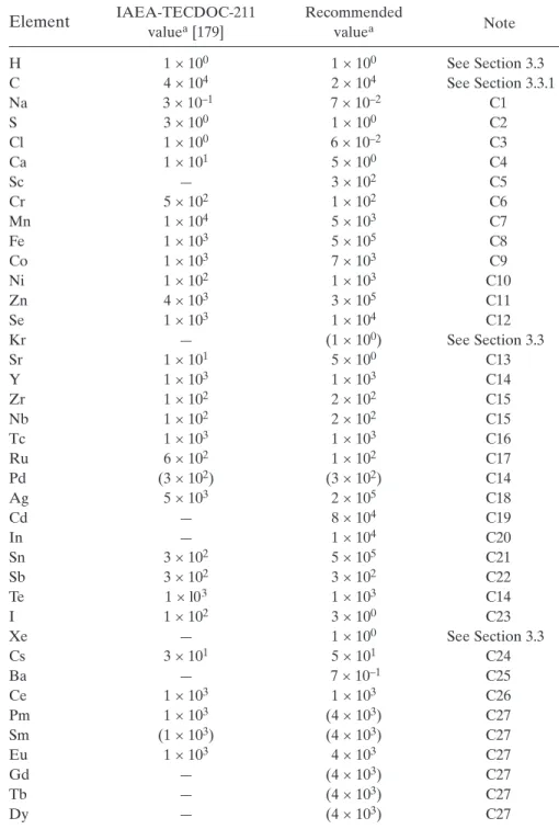
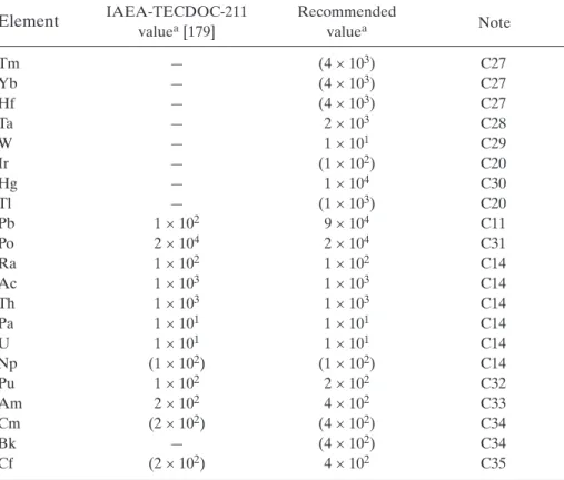
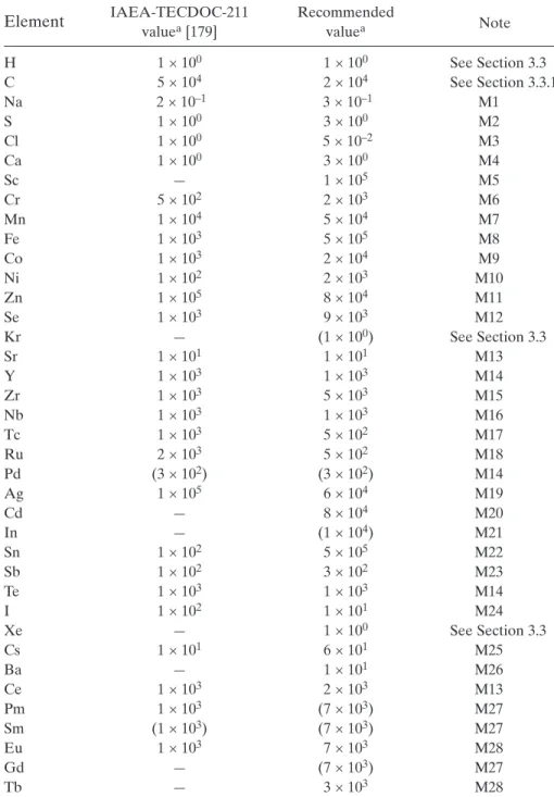
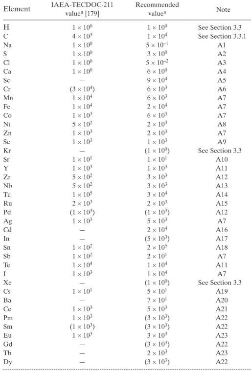
2.2.1. Derivation of open ocean KdsRecommended K
ds for the open ocean environment for a number of ele-
ments are listed in column 2 of Table I. In addition, a selection of K
ds based on
field observations or laboratory experiments has been compiled and is pre-
sented in the last column, where possible using values published in peer
reviewed literature. The remainder of Table I contains the details from which
the recommended values were calculated.
Kd (L/kg) =
Concentration per unit mass of particulate (kg/kkg or Bq/kg dry weight) Concentration per unit volume of waater (kg/L or Bq/L)
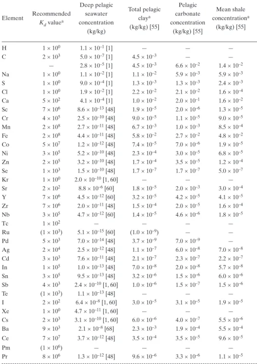
TABLE I. OPEN OCEAN K
ds
Deep pelagic Pelagic
Recommended seawater Total pelagic
carbonate Mean shale Element
Kdvaluea concentration clay
a
concentration concentrationa (kg/kg) (kg/kg) [55]
(kg/kg) [55] (kg/kg) [55]
H 1 × 100 1.1 × 10⁻¹[1] — — —
C 2 × 10³ 5.0 × 10⁻⁷[1] 4.5 × 10⁻³ — —
— 2.8 × 10⁻⁵[1] 4.5 × 10⁻³ 6.6 × 10⁻² 1.4 × 10⁻² Na 1 × 100 1.1 × 10⁻²[1] 1.1 × 10⁻² 5.9 × 10⁻³ 5.9 × 10⁻³ S 1 × 100 9.0 × 10⁻⁴[1] 1.3 × 10⁻³ 1.3 × 10⁻³ 2.4 × 10⁻³ Cl 1 × 100 1.9 × 10⁻²[1] 2.2 × 10⁻² 2.1 × 10⁻² 1.6 × 10⁻⁴ Ca 5 × 10² 4.1 × 10⁻⁴[1] 1.0 × 10⁻² 2.0 × 10⁻¹ 1.6 × 10⁻² Sc 7 × 10⁶ 8.6 × 10⁻¹³[48] 1.9 × 10⁻⁵ 2.0 × 10⁻⁶ 1.3 × 10⁻⁵ Cr 4 × 10⁵ 2.5 × 10⁻¹⁰[48] 9.0 × 10⁻⁵ 1.1 × 10⁻⁵ 9.0 × 10⁻⁵ Mn 2 × 10⁸ 2.7 × 10⁻¹¹[48] 6.7 × 10⁻³ 1.0 × 10⁻³ 8.5 × 10⁻⁴ Fe 2 × 10⁸ 4.4 × 10⁻¹¹[48] 5.8 × 10⁻² 2.7 × 10⁻² 4.8 × 10⁻² Co 5 × 10⁷ 1.2 × 10⁻¹²[48] 7.4 × 10⁻⁵ 7.0 × 10⁻⁶ 1.9 × 10⁻⁵ Ni 3 × 10⁵ 5.2 × 10⁻¹⁰[48] 2.3 × 10⁻⁴ 3.0 × 10⁻⁵ 6.8 × 10⁻⁵ Zn 2 × 10⁵ 3.2 × 10⁻¹⁰[48] 1.7 × 10⁻⁴ 3.5 × 10⁻⁵ 1.2 × 10⁻⁴ Se 1 × 10³ 1.5 × 10⁻¹⁰[48] 1.7 × 10⁻⁷ 1.7 × 10⁻⁷ 5.0 × 10⁻⁷
Kr 1 × 100 2.0 × 10⁻¹⁰[1, 60] — — —
Sr 2 × 10² 8.8 × 10⁻⁶[60] 1.8 × 10⁻⁵ 2.0 × 10⁻³ 3.0 × 10⁻⁴ Y 7 × 10⁶ 4.5 × 10⁻¹²[60] 3.2 × 10⁻⁵ 4.2 × 10⁻⁵ 4.1 × 10⁻⁵ Zr 7 × 10⁶ 2.0 × 10⁻¹¹[48] 1.5 × 10⁻⁴ 2.0 × 10⁻⁵ 1.6 × 10⁻⁴ Nb 3 × 10⁵ 4.7 × 10⁻¹²[60] 1.4 × 10⁻⁵ 4.6 × 10⁻⁶ 1.8 × 10⁻⁵
Tc 1 × 10² — — — —
Ru (1 × 10³) 5.1 × 10⁻¹⁵[60] (1.0 × 10⁻⁹) — —
Pd 5 × 10³ 7.0 × 10⁻¹⁴[48] 3.7 × 10⁻⁹ 7.0 × 10⁻⁹ —
Ag 2 × 10⁴ 2.5 × 10⁻¹²[48] 1.1 × 10⁻⁷ 6.0 × 10⁻⁸ 7.0 × 10⁻⁸ Cd 3 × 10³ 7.6 × 10⁻¹¹[48] 2.1 × 10⁻⁷ 2.3 × 10⁻⁷ 2.2 × 10⁻⁷ In 1 × 10⁵ 1.0 × 10⁻¹³[48] 7.0 × 10⁻⁸ 2.0 × 10⁻⁸ 5.7 × 10⁻⁸ Sn 3 × 10⁵ 9.5 × 10⁻¹³[48] 3.2 × 10⁻⁶ 1.5 × 10⁻⁶ 6.0 × 10⁻⁶ Sb 4 × 10³ 2.4 × 10⁻¹⁰[1, 60] 1.0 × 10⁻⁶ 1.5 × 10⁻⁷ 1.5 × 10⁻⁶
Te (1 × 10³) 1.1 × 10⁻¹³[48] — — —
I 2 × 10² 6.4 × 10⁻⁸[1, 60] 3.0 × 10⁻⁵ 3.1 × 10⁻⁵ 1.9 × 10⁻⁵
Xe 1 × 100 4.7 × 10⁻¹¹[1, 60] — — —
Cs 2 × 10³ 3.1 × 10⁻¹⁰[1, 60] 6.0 × 10⁻⁶ 4.0 × 10⁻⁷ 5.5 × 10⁻⁶ Ba 9 × 10³ 2.1 × 10⁻⁸[68] 2.3 × 10⁻³ 1.9 × 10⁻⁴ 5.5 × 10⁻⁴ Ce 7 × 10⁷ 3.7 × 10⁻¹²[48] 3.5 × 10⁻⁴ 3.5 × 10⁻⁵ 9.6 × 10⁻⁵
Pm (1 × 10⁶) — — — —
Pr 8 × 10⁶ 1.3 × 10⁻¹²[48] 9.6 × 10⁻⁶ 3.3 × 10⁻⁶ 1.1 × 10⁻⁵
Kdbased on Kdbased on Kdbased on Potential clay
total pelagic potential potential enrichment
clay enrichment carbonate Other derived Kds (kg/kg)
(kg/kg) (kg/kg) exchange
(kg/kg)
— — — — —
— 9.0 × 10³ — — —
— 1.6 × 10² — 2.4 × 10³ —
5.1 × 10⁻³ 1.0 × 100 4.6 × 10⁻¹ — 1 × 10⁻¹–2.4 × 100[56, 57]
— 1.4 × 100 — — —
2.2 × 10⁻² 1.2 × 100 1.1 × 100 — —
— 2.4 × 101 — 4.9 × 10² 1 × 10²[56]
6.0 × 10⁻⁶ 2.2 × 10⁷ 7.0 × 10⁶ — 4 × 10⁷–5 × 10⁷[56, 58]
— 3.6 × 10⁵ — — 3 × 10⁵–5 × 10⁵[56, 58]
5.9 × 10⁻³ 2.5 × 10⁸ 2.2 × 10⁸ — 8 × 10⁶–2 × 10⁷[4, 57, 58] 1.0 × 10⁻² 1.3 × 10⁹ 2.3 × 10⁸ — 5 × 10⁵–5 × 10⁷[4, 57, 58] 5.5 × 10⁻⁵ 6.2 × 10⁷ 4.6 × 10⁷ — 1 × 10⁶–6 × 10⁶[4, 57, 58] 1.6 × 10⁻⁴ 4.5 × 10⁵ 3.1 × 10⁵ — 3 × 10⁵–5 × 10⁵[56, 58] 5.0 × 10⁻⁵ 5.3 × 10⁵ 1.6 × 10⁵ — 1 × 10⁵–4 × 10⁵[56–58]
— 1.1 × 10³ — — 8 × 10²–1 × 10⁴[57–59]
— — — — —
— 2.0 × 100 — 2.5 × 10² 1 × 10⁻¹[56]
— 7.1 × 10⁶ — — 8 × 10⁷[56]
— 7.4 × 10⁶ — — 8 × 10⁶[56]
— 3.0 × 10⁶ — — —
— — — — 1 × 100–1 × 101[61–66]
— (2.0 × 10⁵) — — —
— 5.3 × 10⁴ — — —
4.0 × 10⁻⁸ 4.4 × 10⁴ 1.6 × 10⁴ — 3 × 10³–5 × 10³[56, 58]
— 2.8 × 10³ — — 9.5 × 101–1 × 10⁴[56–58]
1.3 × 10⁻⁸ 6.7 × 10⁵ 1.3 × 10⁵ — 1 × 10⁶[56]
— 3.4 × 10⁶ — — 1 × 10⁵[57]
— 4.1 × 10³ — — 5 × 10³–2.1 × 10⁴[57, 58]
— — — — —
1.1 × 10⁻⁵ 4.7 × 10² 1.7 × 10² — 1 × 10²–1.3 × 10⁴[59, 67]
— — — — —
5.0 × 10⁻⁷ 2.0 × 10⁴ 1.6 × 10³ — 4 × 10²–2 × 10⁴[56–58] 1.8 × 10⁻³ 1.1 × 10⁵ 8.3 × 10⁴ 9.0 × 10³ 2 × 10⁴–1 × 10⁵[56, 57]
2.5 × 10⁻⁴ 9.4 × 10⁷ 6.8 × 10⁷ — 1 × 10⁸[56]
— (1.0 × 10⁷) — — —
— 7.6 × 10⁶ — — 2 × 10⁷[56]
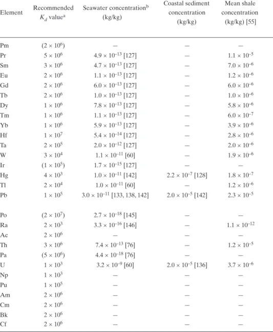
TABLE I. (cont.)
Deep pelagic Pelagic
Recommended seawater Total pelagic
carbonate Mean shale Element
Kdvaluea concentration clay
a
concentration concentrationa (kg/kg) (kg/kg) [55]
(kg/kg) [55] (kg/kg) [55]
Sm 5 × 10⁵ 1.2 × 10⁻¹²[48] 6.2 × 10⁻⁶ 3.8 × 10⁻⁶ 7.0 × 10⁻⁶ Eu 2 × 10⁶ 3.0 × 10⁻¹³[48] 1.8 × 10⁻⁶ 6.0 × 10⁻⁷ 1.2 × 10⁻⁶ Gd 7 × 10⁵ 2.0 × 10⁻¹²[48] 7.4 × 10⁻⁶ 3.8 × 10⁻⁶ 6.0 × 10⁻⁶ Tb 4 × 10⁵ 2.7 × 10⁻¹³[48] 1.1 × 10⁻⁶ 6.0 × 10⁻⁷ 1.0 × 10⁻⁶ Dy (5 × 10⁶) 9.1 × 10⁻¹³[48] (6.0 × 10⁻⁶) 2.7 × 10⁻⁶ 5.8 × 10⁻⁶ Tm 2 × 10⁵ 2.9 × 10⁻¹³[48] 5.6 × 10⁻⁷ 1.0 × 10⁻⁷ 6.0 × 10⁻⁷ Yb 2 × 10⁵ 1.9 × 10⁻¹²[48] 2.9 × 10⁻⁶ 1.5 × 10⁻⁶ 3.9 × 10⁻⁶ Hf 6 × 10⁶ 2.1 × 10⁻¹³[48] 4.1 × 10⁻⁶ 4.1 × 10⁻⁷ 2.8 × 10⁻⁶ Ta 5 × 10⁴ 2.4 × 10⁻¹²[48] 1.2 × 10⁻⁶ 1.0 × 10⁻⁸ 2.0 × 10⁻⁶ W 1 × 10³ 1.0 × 10⁻¹⁰[1, 60] 1.1 × 10⁻⁶ 1.1 × 10⁻⁷ 1.9 × 10⁻⁶ Ir (3 × 10⁶) 1.7 × 10⁻¹⁵[48] 3.0 × 10⁻¹⁰ — (3.0 × 10⁻¹²) Hg 3 × 10⁴ 2.5 × 10⁻¹³[60] 8.0 × 10⁻⁸ 4.6 × 10⁻⁷ 1.8 × 10⁻⁷ Tl 9 × 10⁴ 1.0 × 10⁻¹¹[1, 60] 9.0 × 10⁻⁷ 1.6 × 10⁻⁷ 1.2 × 10⁻⁶ Pb 1 × 10⁷ 4.0 × 10⁻¹²[1, 60] 8.0 × 10⁻⁵ 1.7 × 10⁻⁵ 2.3 × 10⁻⁵
Po (2 × 10⁷) 2.3 × 10⁻¹⁸[60] — — —
Ra 4 × 10³ 5.6 × 10⁻¹⁶[69, 70] 2.0 × 10⁻¹¹ 2.0 × 10⁻¹² 1.1 × 10⁻¹²
Ac (2 × 10⁶) 6.9 × 10⁻²⁰[60] — — —
Th 5 × 10⁶ 1.0 × 10⁻¹³[1, 72] 5.0 × 10⁻⁶ 1.0 × 10⁻⁶ 1.2 × 10⁻⁵
Pa (5 × 10⁶) 1.7 × 10⁻¹⁷[76] — — —
U 5 × 10² 3.2 × 10⁻⁹[1, 60] 1.0 × 10⁻⁶ 1.6 × 10⁻⁶ 3.7 × 10⁻⁶
Np 1 × 10³ — — — —
Pu 1 × 10⁵ — — — —
Am 2 × 10⁶ — — — —
Cm 2 × 10⁶ — — — —
Bk (2 × 10⁶) — — — —
Cf (2 × 10⁶) — — — —
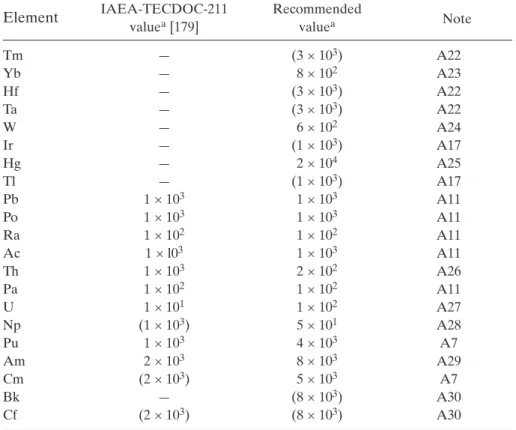
aValues in parentheses indicate that data are insufficient to calculate Kds using the methodology described in Section 2.2.1 and therefore the recommended values were chosen to be equal to the Kds of periodically adjacent elements.
Kdbased on Kdbased on Kdbased on Potential clay
total pelagic potential potential enrichment
clay enrichment carbonate Other derived Kds (kg/kg)
(kg/kg) (kg/kg) exchange
(kg/kg)
— 5.1 × 10⁶ — — —
6.0 × 10⁻⁷ 5.9 × 10⁶ 2.0 × 10⁶ — —
1.4 × 10⁻⁶ 3.8 × 10⁶ 7.1 × 10⁵ — —
1.0 × 10⁻⁷ 4.0 × 10⁶ 3.6 × 10⁵ — —
2.0 × 10⁻⁷ (6.6 × 10⁶) (2.2 × 10⁵) — —
— 1.9 × 10⁶ — — —
— 1.5 × 10⁶ — — —
1.3 × 10⁻⁶ 2.0 × 10⁷ 6.3 × 10⁶ — 1 × 10⁶[56]
— 5.1 × 10⁵ — — —
— 1.1 × 10⁴ — — —
— (1.8 × 10⁵) — — —
— 3.2 × 10⁵ — — 3 × 10³–5 × 10³[56, 58]
— 9.0 × 10⁴ — — 1 × 10⁵[56]
5.7 × 10⁻⁵ 2.0 × 10⁷ 1.4 × 10⁷ — 1 × 10⁴–5 × 10⁷[4, 56, 59]
— — — — —
1.9 × 10⁻¹¹ 3.6 × 10⁴ 3.4 × 10⁴ 3.6 × 10³ 5 × 10²[59]
— — — — —
— 4.9 × 10⁷ — — 1 × 10⁵–1 × 10⁷[4, 56, 58,
59, 71, 73–75]
— — — — 1 × 10⁴–1 × 10⁷[4, 59]
— 3.1 × 10² — 5.0 × 10² 5 × 10²[56, 58, 59]
— — — — 1 × 10²–5 × 10⁴
(see Section 2.2.2)
— — — — 1 × 10⁴–1 × 10⁶
(see Section 2.2.2)
— — — — 1 × 10⁵–2 × 10⁷
(see Section 2.2.2)
— — — — —
— — — — —
— — — — —
The recommended K
ds (column 2) are based on the estimate of pelagic
clay enrichment in relation to source rocks. Where no such enrichment is
indicated, it has been assumed, arbitrarily, that 10% of the total pelagic clay
abundance represents the proportion of exchangeable phase particulate ele-
ment. The only exceptions to this procedure are where the experimental
measurements, presented in the table, suggest that the K
dis closer to the value
based on the total pelagic clay concentration than to the value based on 10%
of this concentration (Sc, Cr, Se, Y, Zr, Cd, Sb, Pr and Tl).
Deep water dissolved element concentrations (column 3) represent, in
most instances, the mean of Atlantic and Pacific values taken from the most
reliable and recent sources. This is a departure from TRS 247, in which North
Atlantic values were preferentially used. The dissolved concentrations were
based on either analysis of filtered samples of sea water or, for trace con-
stituents, analysis of the acid soluble fraction of unfiltered samples of sea water.
For aluminum, iron and manganese the concentrations given in Table I are
those resulting from analysis of filtered samples of sea water, as unfiltered sea
water contains significant additional colloidal and fine particulate contribu-
tions of these elements.
The detailed calculation was as follows. The concentrations of the ele-
ments in pelagic clay (column 4), pelagic carbonate sediments (column 5) and
mean shales (column 6) were derived from Bowen [55]. The ratio of the con-
centration of an element in pelagic clays to that in deep ocean water provides
one estimate of the K
d(column 8) for the element. Several authors have
reported marine elemental mass balances, and the partitioning of elements
between various marine phases was determined on this basis [56, 58, 77–81].
However, for the purpose of deriving suitable K
ds for use in oceanographic and
radiological models applied to the transport of radioactive waste, an estimate
of the wholly exchangeable particulate phase component is needed. This was
estimated from the difference between the total pelagic clay element concen-
tration and the source rock abundance. Where this difference is positive it has
been assumed to be a measure of the augmentation of pelagic clays by authi-
genic components during transport between weathering and sedimentation. In
very few cases does the crude estimate of potentially exchangeable element
concentration depend on whether shale or mean crustal abundances have been
used to subtract detrital (crystalline) phase concentrations from total pelagic
clay concentrations; such cases are those of selenium, mercury and thallium.
For all three, the mean crustal abundance provides the greater estimate of
exchangeable phase concentration. The mean shale was used as the basis for
assessing pelagic clay enrichment. Where the difference between pelagic clay
and mean shale concentrations is positive, suggesting that pelagic clay sedi-
ments are enriched over source rock abundance, the difference is shown in
column 7 of Table I. This value was subsequently divided by the seawater con-
centration to yield a value of K
dbased on potential pelagic clay enrichment
(column 9). Where the difference between pelagic clay and source rock abun-
dance is zero or negative, no entry appears in column 7 and the estimate of the
Kdis provided by dividing the total pelagic clay concentration by the seawater
concentration (column 8).
The recommended K
ds for elements that are primary constituents of cal-
careous biogenic material (Ca, Sr, Ba, Ra and U) were derived from the K
ds
based on potential carbonate exchange (column 10), which were determined
from the ratio of the concentrations in calcareous pelagic sediments (column 5)
to those in deep pelagic water (column 3). A K
dis also provided in column 10
for carbon, based on the ratio of carbon in carbonaceous sediments to that in
dissolved organic and carbonate forms in sea water.
2.2.2. Alternative derivation of Kds: review of published data
Experimental and field data published in the literature were reviewed to
compare them with the K
ds derived using the methodology described in
Section 2.2.1 and to determine K
ds for those elements for which such a
methodology could not be applied. This approach was adopted, in particular,
for those nuclides of elements no longer occurring naturally on Earth, which
were introduced into the environment from nuclear activities, such as tech-
netium and the transuranics.
Difficulty is frequently experienced in relating K
ds derived under exper-
imentally controlled conditions with those measured using marine environ-
mental samples. The considerable ranges of experimental K
ds reported for
some elements [82–88] are often a direct result of variations in the materials
and/or procedures adopted. Factors that can significantly influence the appar-
ent K
dinclude: the solid to liquid ratio; the initial concentrations of tracer and
carrier in solution; the pH of the liquid before and after equilibration with the
solids; the grain size of the solids; the time allowed for equilibration; the proce-
dure used for separating the two phases (e.g. filtering or decanting); whether
samples are shaken or left to stand; the phase(s) used to estimate the K
d(fre-
quently only one phase is measured); loss of tracer on container walls or filters;
and competition from other ions in solution. In many cases, particularly those
studies related to radionuclide migration through rock and fractured media,
lack of control of one or more of the above factors, or use of experimental con-
ditions far removed from those found in the marine environment, hinder the
adoption of experimentally derived K
ds for ocean disposal models.
Experimentally derived K
ds were therefore only considered whenever few, or
no, environmental data exist.
For technetium, the recommended K
d(1 × 10
2) is based on environ-
mentally derived values from the Irish Sea [71]. Although they may accurately
reflect the partitioning between
99Tc and the sedimentary material in that
area, the extent to which water and sediments are in equilibrium is not
known. It should not be inferred that the K
ds obtained are universally appli-
cable. In particular, the influence of organic material, such as that arising from
benthic algae, has not been determined. Early experimental studies suggested
that technetium, in either the reduced or oxidized form, generally exhibits a
Kdof less than 10 [61–66]. In the absence of further particulate data, it is
therefore suggested that the recommended value represents an upper bound
in oxic systems.
Neptunium K
ds for suspended sediment in coastal waters of the UK [89,
90] and for sediment pore water in the Irish Sea [71] have been reported.
Experimental K
ds for northeast Atlantic calcareous ooze and clay fall within
this range [91, 92]. Other reported experimental values, for various substrates,
are much lower and are not directly applicable [66, 93, 94].
The recommended K
dfor plutonium is for a mixture of oxidation states
(i.e. Pu III/IV plus V/VI). A relatively large number of environmental K
ds have
been reported from a wide variety of marine, riverine and lacustrine environ-
ments, and they consistently fall within the range 1 × 10
4–1 × 10
6[47, 71,
95–107]. There seems to be little justification in extending the range for sensi-
tivity analysis. A large number of experimental determinations have also been
made, and with very few exceptions (e.g. approximately 1 × 10
1–1 × 10
4for
North Pacific red clays [108]) K
ds fall within the range 1 × 10
4–1 × 10
6[71, 86,
92, 109–114]. The latter range also includes values for calcareous sediments
from the northeast Atlantic [71, 92].
Environmental K
ds for americium and curium are given by Pentreath et
al. [101, 102], Lovett (unpublished data) [106], Aarkrog et al. [104] and Noshkin
(unpublished data) [107]. Few experimental data are available for curium,
although Erickson [108] gives values for abyssal red clays. Far more experi-
mental data are available for americium, with most studies reporting values in
the range of the field data [86, 92, 108, 113–116].
A default K
dof 1 was assigned to non-reactive elements such as hydrogen,
the major elements in sea water (Na, Cl and S) and inert gases (Kr and Xe).
For some elements (Ru, Te, Pm, Dy and Ir) insufficient data are available
to calculate K
ds using the methodology described in Section 2.2.1 or to derive
Kds from published data. The recommended K
ds for these elements were cho-
sen to be equal to K
ds for periodically adjacent elements and appear in paren-
theses in Table I.
From experimental studies it is assumed that trivalent californium
behaves like curium and americium [117, 118].
The oceanic distribution of
210Po is influenced by biological recycling in
surface waters, and
210Po/
210Pb disequilibria have been reported [119].
However, over the whole water column,
210Po and
210Pb are in balance with
respect to their partitioning between water and particulate fractions [120], and
their respective K
ds should be similar. Ranges of K
dwere determined from the
data of Brewer et al. [79, 121] and Whitfield and Turner [122]. Ocean margin
Kds for polonium are assumed to be identical to open ocean values.
Protactinium behaves in a similar fashion to thorium in the open ocean.
Values for the Panama and Guatemala Basins, and for the North Pacific, have
been reported [123, 124]. The K
dappears to correlate with the manganese con-
tent, and scavenging is enhanced at ocean margins. Coastal sediment CFs
should be similar to those of the open sea.
2.2.3. Maximum and minimum values for open ocean Kds