本文総合研究大学院大学学術情報リポジトリ甲1589 本文

(1)

Cosmological tests of models for the accelerating

universe in terms of inhomogeneities

Keiki Saito

DOCTOR OF PHILOSOPHY

Department of Particle and Nuclear Physics

School of High Energy Accelerator Science

The Graduate University for Advanced Studies

2012

(2)

Abstract

We study cosmological tests of models that can explain the apparent accelerated expansion of the present universe. In this thesis, we provide methods of testing these models by particularly focusing on inhomogeneities of the universe, because, practically, our universe is inhomogeneous.

First, we consider the effective gravitational stress-energy tensor for short-wavelength perturbations in modified gravity theories in the cosmological context. We address this problem in a simple class of f (R) gravity theories on the assumptions that (i) the background, or coarse-grained metric averaged over several wavelengths, has the Friedmann- Lemaˆıtre-Robertson-Walker symmetry and that (ii) when our f (R) theory reduces to Ein- stein gravity, the field equations of Einstein gravity should be reproduced. We show by explicit computation that the effective gravitational stress-energy tensor for a cosmological model in our f (R) theories, as well as that obtained in the corresponding scalar-tensor theory, takes a similar form to that in general relativity and is in fact traceless, hence acting again like a radiation fluid as in the case of general relativity. If the assumption (ii) above is dropped, then an undetermined integration constant appears and the resul- tant effective stress-energy tensor acquires a term that is in proportion to the background metric, hence being, in principle, able to describe a cosmological constant. Whether this effective cosmological constant term is positive and whether it has the right magnitude as dark energy depends upon the value of the integration constant.

Second, we discuss temperature anisotropies of cosmic microwave background (CMB) in local void models. We derive analytic formulae for the dipole and quadrupole moments of the CMB temperature anisotropy that hold for any spherically symmetric universe model and can be used to compare consequences of this model with observations of the CMB temperature anisotropy rigorously. We check that our formulae are consistent with the numerical studies previously made for the CMB temperature anisotropy in the void model. We also update the constraints concerning the location of the observers in the void model by applying our analytic dipole formula with the latest WMAP data.

(3)

List of Figures

2.1 Hubble diagrams of SuperNova Legacy Survey (SNLS) and nearby SNe Ia . 22 2.2 (ΩΛ0, Ωm0) and (w, Ωm0) obtained with the Union08 . . . 23 2.3 (ΩM0, w) plane from SN Ia combined with the constraints from BAO and

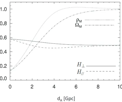
CMB . . . 26 3.1 The radial dependence of ρm, Ωm, H⊥ and H// in the GBH model . . . 48

(7)

Chapter 1 Introduction

In modern cosmology, it is commonly assumed that our universe be isotropic and homogeneous on sufficiently large scales under the cosmological principle, and accordingly be described by the Friedmann-Lemaˆıtre-Robertson-Walker (FLRW) metric as a first approximation. Then, together with consequences of various cosmological observations such as the power spectrum of Cosmic Microwave Background (CMB) temperature anisotropy, the distance-redshift relation of SuperNova of type Ia (SN Ia) indicates that the expansion of the present universe is apparently accelerated as first observed in 1998 [1, 2].

In general relativity, if the universe is filled with ordinary non-relativistic matter and radiation that are the two known constituents of the universe, then gravity should lead to a slowing of the expansion. Since the expansion is apparently accelerated, there are three possibilities, any of which would have deep implications for our understanding of the universe and theory of gravity. The first is that about 75% of the energy density of the universe exists in a new form, known as “dark energy” which has negative pressure. However, there does not appear to be any satisfactory theory that can naturally explain the origin of dark energy and its magnitude required by observations. The second is that general relativity is broken on cosmological scales and must be replaced with a more appropriate theory of gravity, i.e., “modified gravity theory.” The third is that the assumption that the universe is homogeneous breaks down, having instead an under-dense local void in the surrounding overdense universe, so-called “local void model.”

We can regard the so-called cosmological constant Λ whose equation of state is w_DE =

(8)

−1 as the simplest candidate for dark energy. If the cosmological constant originates from a vacuum energy of particle physics, its energy scale is significantly larger than the observed value of the present dark energy density [3]. We need to find a mechanism to obtain the tiny value of Λ consistent with observations.

To understand the property of dark energy, we should first clarify whether it is a simple constant or it dynamically changes in time. The dynamical dark energy models can be distinguished from the cosmological constant by considering the time evolution of wDE. A wide variety of variations of wDE is predicted by the scalar field models, such as quintessence [4, 5] and k-essence [6–8]. Still, the current observational data are not sufficient to provide some preference of such models over the Λ-Cold Dark Matter (ΛCDM) model. Furthermore, the field needs to have sufficiently flat potentials such that the field evolves slowly enough to drive the accelerated expansion of the present universe. This demands that the field mass is extremely small relative to typical mass scales appearing in particle physics [9, 10]. It seems to be an extremely difficut task to construct viable scalar field dark energy models within the framework of particle physics. There exists another class of dynamical dark energy models based on the large-distance modification of gravity, for example, f (R) gravity [11], scalar-tensor theories, Gauss- Bonnet gravity [12, 13], Dvali-Gabadadze-Porrati (DGP) braneworld model [14], and so on. An attractive feature of these models is that the cosmic acceleration can be realized without introducing dark energy for matter contents of the universe. There are tight constraints coming from local gravity tests by modifying general relativity. Hence, in general, the restriction on modified gravity theories is stringent compared to modified matter models.

Among many, one of the simplest of modified theories so far proposed is the so- called f (R) gravity, whose action is a generalization of the Einstein-Hilbert action to an arbitrary function, f (R), of the scalar curvature R. For example, an f (R) model of the form f (R) = R − µ²⁽ⁿ⁺¹⁾^/Rⁿ (n > 0) was proposed to explain the late-time cosmic acceleration [15, 16]. However, this model suffers from a number of problems such as the incompatibility with local gravity constraints [17, 18], the instability of density perturbations [19, 20], and the absence of a matter-dominated epoch [21, 22]. As we will see in this thesis there are a number of conditions required for the viability of f (R) dark

(9)

energy models [23–25], which stimulated to propose viable models [26–28]. It is well known that f (R) gravity is equivalent to a scalar-tensor theory which contains the coupling of the scalar curvature R to a scalar field ϕ in a certain way [17]. Brans-Dicke theory [29] is one of the simplest examples.

In addition to the scalar curvature R, we can construct other scalar quantities such as RµνR^µν and RµνλσR^µνλσ from the Ricci tensor Rµν and Riemann tensor Rµνλσ [30]. For the Gauss-Bonnet curvature invariant defined by G ≡ R² − 4Rµν^R^µν^{+ R}µνλσ^R^µνλσ^,

it is known that we can avoid the appearance of spurious spin-2 ghosts [31]. In order to give rise to some contribution of the Gauss-Bonnet term to the Friedmann equation, we require that (i) the Gauss-Bonnet term couples to a scalar field ϕ, i.e., F (ϕ)G or (ii) the Lagrangian density f is a function of G, i.e., f(G). We shall review such theories and observational constraints on them.

In DGP braneworld model, we consider a 3-dimensional brane embedded in the 5- dimensional Minkowski bulk spacetime [14]. The gravitational leakage to the extra dimen- sion leads to a self-acceleration of the universe on the 3-dimensional brane. A longitudinal graviton (i.e. a branebending mode ϕ) gives rise to a nonlinear self-interaction of the form (r²_c/m_pl_)□ϕ∂^µϕ∂_µϕ through the mixing with a transverse graviton, where r_cis a cross-over scale (of the order of the Hubble radius H₀⁻¹ today) and mpl is the Planck mass [32]. In the local region where the energy density ρ is much larger than r_c⁻²m²_pl, the nonlinear self-interaction can lead to the decoupling of the field from matter through the so-called Vainshtein mechanism [33], which allows a possibility for the consistency with local gravity constraints. However, the DGP braneworld model suffers from a ghost problem [34], in addition to the difficulty for satisfying the combined observational constraints.

In addition to the above mentioned models, there are attempts to explain the cosmic acceleration without dark energy. One of such attempts is the local void model proposed by Tomita [35, 36], also independently by Celerier [37] and by Goodwin et al. [38]. In this model, our universe is no longer assumed to be homogeneous, having instead an under-dense local void in the surrounding overdense universe. The isotropic nature of cosmological observations on large scales is realized by assuming the spherical symmetry and demanding that we live close to the center of the void. Furthermore, the model is supposed to contain only ordinary dust like cosmic matter, describing, say, CDM component. Such

(10)

a spacetime can be described by the Lemaˆıtre-Tolman-Bondi (LTB) spacetime [39–41]. Since the rate of expansion in the void region is larger than that in the outer overdense region, this model can account for the observed dimming of SN Ia luminosity. In fact, recent numerical analyses [42–52] have shown that the LTB model can accurately repro- duce the SN Ia distance-redshift relation. For this reason, despite the relinquishment of the widely accepted Copernican/cosmological principle, the local void model has recently attracted considerable attention.

Another example is the so-called backreaction model in which the backreaction of spatial inhomogeneities on the FLRW background is responsible for the real acceleration. Our observable universe appears to be homogeneous and isotropic on large scales, but highly inhomogeneous on small scales. It is therefore interesting to consider whether the local inhomogeneities can have any effects on the global dynamics of our universe, in particular, any effect that corresponds to a positive cosmological constant or dark energy. A number of authors have explored this possibility of explaining the present cosmic accelerating expansion by some backreaction effects of the local inhomogeneities [53–61]. Such a backreaction effect may be described in terms of an effective stress-energy tensor arising from metric as well as matter perturbations.

In this thesis, we discuss cosmological tests of modified gravity theories and the local void model in terms of inhomogeneities of the universe. We first consider backreaction of inhomogeneities and effective stress energy tensor in f (R) gravity (Chapter 5) and then consider off-center CMB anisotropies in local void models (Chapter 6).

In Chapter 5, the high frequency limit in f (R) gravity and scalar-tensor theory is studied [62]. In general relativity, a consistent expansion scheme for short-wavelength perturbations and the corresponding effective stress-energy tensor were largely developed by Isaacson [63, 64], in which the small parameter, say ϵ, corresponds to the amplitude and at the same time the wavelength of perturbations. Isaacson’s expansion scheme is called the high frequency limit or the short-wavelength approximation. If the effective stress-energy tensor had a term proportional to the background spacetime metric, then it would correspond to adding a cosmological constant to the effective Einstein equations for the background metric, thereby explaining possible origin of dark energy from local inhomogeneities. It has been shown, however, that this effective gravitational stress-

(11)

energy tensor is traceless and satisfies the weak energy condition, i.e. acts like radiation [65,66], and thus cannot provide any effects that imitate dark energy in general relativity. However, it is far from obvious if this traceless property of the effective gravitational stress-energy tensor is a nature specific only to the general relativity or is rather a generic property that can also hold in other types of gravity theories.

The purpose of Chapter 5 is to address this question in a simple, concrete model in the cosmological context. Since f (R) gravity contains higher-order derivative terms, one can anticipate the effective gravitational stress-energy tensor to be generally modified in the high frequency limit. Our analysis can be performed, in principle, either (i) by first translating a given f (R) gravity into the corresponding scalar-tensor theory and then inspecting the stress-energy tensor for the scalar field ϕ, or (ii) by directly dealing with metric perturbations of f (R) gravity. We may expect that the former approach is sufficient for our present purpose and much easier than the latter metric approach, as we have to deal with metric perturbations of complicated combinations of the curvature tensors in the latter case. Nevertheless, we will take both approaches. In fact, in the metric approach, by directly taking up perturbations of the scalar curvature R, the Ricci tensor R_µν and the Riemann tensor R^µ_νλσ involved in a given f (R) theory, we can learn how to generalize our present analysis of a specific class of f (R) gravity to analyses of other, different, types of modified gravity theory that cannot even be translated into a scalar-tensor theory, such as the Gauss-Bonnet gravity. Then, we will make sure that the effective stress-energy tensor in Brans-Dicke theory is consistent with that in our f (R) gravity.

In Chapter 6, we turn to the local void model. In order to justify the local void model as a viable alternative to the standard ΛCDM model, we have to test this model by various observations other than the SN Ia distance-redshift relation. Most of previous analyses were performed for various types of local void models by using numerical methods, and it does not seem to be straightforward to compare analyses for each different model so as to have a coherent understanding of the results. In order to have general consequences of the local void model and systematically examine its viability, it is desirable to develop some general, analytic methods that can apply, independently of the details of each specific model.

(12)

The purpose of Chapter 6 is to derive the analytic formulae for the dipole and quadrupole of the CMB anisotropy in general spherically symmetric spacetimes, including the Λ-LTB spacetime, and to give constraints on the local void model. We will exploit the key requirement of the local void model that we, observers, are restricted to be around very near the center of the spherical symmetry: Namely, we first note that the small distance between the symmetry center and an off-center observer gives rise to a corresponding deviation in the photon distribution function. Then, by taking ‘Taylor-expansions’ of the photon distribution function at the center with respect to the deviation, we can read off the CMB temperature anisotropy caused by the deviation in the photon distribution function. By doing so, we can, in principle, construct the l-th order multiple moment of the CMB temperature anisotropy from the (up to) l-th order expansion coefficients, with the help of the background null geodesic equations and the Boltzmann equation. We will do so for the first and second-order expansions to find the CMB dipole and quadrupole moments. We also provide the concrete expression of the corresponding formulae for the local void model. Our formulae are then checked to be consistent with the numerical analyses of the CMB temperature anisotropy in the local void model, previously made by Alnes and Amarzguioui [47]. We apply our formulae to place the constraint on the distance between an observer and the symmetry center of the void, by using the latest Wilkinson Microwave Anisotropy Probe (WMAP) data, thereby updating the results of the previous analyses.

This thesis is organized as follows. In Chapter 2, we briefly review the FLRW cosmology and provide recent observational constraints on dark energy obtained from SN Ia, CMB and Baryon Acoustic Oscillations (BAO) data. Moreover, we introduce the cosmological constant Λ and the cosmological constant problem. In Chapter 3, we summarize current theoretical approaches to accelerated expansion and dark energy, including modified matter models, modified gravity theories, the local void model. In Chapter 4, we provide a number of ways to distinguish modified gravity theories and the local void model observationally from the ΛCDM model, and some constraints on these models. Chapter 5 and Chapter 6 are the main parts of this thesis. Chapter 7 is devoted to a summary and discussion.

Our signature convention for g_µν is (−, +, +, +). We define the Riemann tensor by

(13)

R_µνλ^σω_σ _{= 2∇}_[µ_∇_ν]ω_λ and the Ricci tensor by R_µν = R_µλν^λas in Wald’s book [68]. We use units such that c = ℏ = 1, where c is the speed of light and ℏ is reduced Planck^’s constant. The gravitational constant G is related to the Planck mass m_pl = 1.2211 × 10¹⁹ ^{GeV via} G = 1/m²_pland the reduced Planck mass Mpl= 2.4357×10¹⁸ ^{GeV via κ}² = 8πG = 1/M_pl², respectively.

(14)

Chapter 2 Apparent accelerated expansion of

the present universe

2.1 FLRW cosmology

2.1.1 Isotropic and homogeneous universe

FLRW spacetime

Our observable universe appears to be isotropic and homogeneous on large scales and accordingly be described by the Friedmann-Lemaˆıtre-Robertson-Walker (FLRW) metric:

gµνdx^µdx^ν _{= −dt}²+ a²(t)γijdxⁱdx^j

= −dt²^{+ a}²^(t)

{ dr²

1 − Kr² ^{+ r}

2_(dθ2_{+ sin}2_θdϕ2⁾

}

, (2.1.1)

where a(t) is cosmic scale factor with cosmic time t. The coordinates r, θ and ϕ are known as comoving coordinates. The spatial curvature constant K describes the geometry of the spatial section. It may be convenient to write the metric (2.1.1) in the following form:

gµνdx^µdx^ν _{= −dt}²+ a²(t){dχ²+ f_K²(χ)(dθ²+ sin²θdϕ²)} , (2.1.2)

(15)

where

fK(χ) =











sin χ (K > 0); closed χ (K = 0); flat sinh χ (K < 0); open.

(2.1.3)

Note that (2.1.1) is invariant under the scaling a(t) → ξa(t), r → r/ξ, K → ξ²^{K, where} ξ is an arbitrary constant. This allows us to normalize k or a(t) arbitrarily. We can set

a(t0_{) ≡ 1,} (2.1.4)

where a subscript 0 means the present value.

The stress-energy tensor of the isotropic and homogeneous universe should take the same form as for a perfect fluid [69]:

Tµν = (ρ + P )UµUν + P gµν, (2.1.5)

where ρ = ρ(t) and P = P (t) are the energy density and the pressure density of the fluid, respectively, and U^µ _{≡ dx}^µ/dt is the four-velocity with U^µUµ = −1. With one index raised, the stress-energy tensor takes the convenient form:

T^µ_ν = diag(−ρ, P, P, P ). ^(2.1.6)

The Einstein field equation reads

Gµν _{≡ R}µν ₋

1

2^Rg^µν ^{= 8πGT}^µν^, ^(2.1.7)

where Gµν is the Einstein tensor, Rµν is the Ricci tensor and R ≡ R^µ^µ is the scalar curvature. In the FLRW background (2.1.1), the Einstein equation gives the Friedmann equations

H² = ^8πG 3 ^{ρ −}

K

a²^, ^(2.1.8)

¨ a

a ^{= −}

4πG

3 (ρ + 3P ) , (2.1.9)

(16)

where dot denotes a derivative with respect to t, and

H(t) ≡ _a(t)^˙a(t) ^(2.1.10)

is the Hubble parameter which characterizes the rate of cosmic expansion. The value of the Hubble parameter at the present epoch is the Hubble constant, H0. Current observations lead us to believe that the Hubble constant is 73.8 ± 2.4 km/sec/Mpc [70]. (Mpc stands for megaparsec, which is 3.09 × 10²⁴ cm.) Since there is still some uncertainty in this value, we often parametrize the Hubble constant as

H0 = 100h km/sec/Mpc, (2.1.11)

so that h ≈ 0.7.

Equation (2.1.8) can be rewritten

Ω − 1 = _H^K₂_a₂^, ^(2.1.12)

where Ω ≡ ρm^/ρc is the dimensionless density parameter and ρ_c is the critical density defined by

ρ_c_≡ ^3H

2

8πG^. ^(2.1.13)

The density parameter tell us which of the three spatial geometries describes our universe, i.e.,

ρ > ρc ↔ Ω > 1 ↔ K > 0 ↔ closed ρ = ρc ↔ Ω = 1 ↔ K = 0 ↔ flat ρ < ρc ↔ Ω < 1 ↔ K < 0 ↔ open.

(2.1.14)

Recent observations of the cosmic microwave background (CMB) anisotropy have shown that the current universe is very close to a spatially flat geometry (Ω ≃ 1) [71]. This is actually a natural result from inflation in the early universe [72]. Hence, we will consider a flat universe (K = 0) as necessary.

The stress-energy tensor is conserved by virtue of the Bianchi identities, leading to

(17)

the continuity equation

˙ρ = −3H(ρ + P ). ^(2.1.15)

This equation can be derived from (2.1.8) and (2.1.9), which means that two of equations (2.1.8), (2.1.9) and (2.1.15) are independent.

Evolution of the scale factor

Let us consider the evolution of the universe filled with a barotropic perfect fluid with an equation of state

P = wρ. (2.1.16)

By solving (2.1.15), we obtain

ρ ∝ exp [

−3

∫ a

da1

a1

(1 + w(a1)) ]

. (2.1.17)

When w is assumed to be constant, this can be integrated to derive

ρ ∝ a^−3(1+w)^. ^(2.1.18)

The two most popular examples of cosmological fluids are known as non-relativistic matter (w = 0) and radiation (w = 1/3). The energy densities in the matter or radiation dominated universe are

ρm _{∝ a}⁻³ : matter, (2.1.19)

ρr _{∝ a}⁻⁴ : radiation. (2.1.20)

Solving the Friedmann equation (2.1.8) with K = 0 and (2.1.18) yields

a ∝ (t − t⁰⁾^3(1+w)² ^. ^(2.1.21)

(18)

The scale factors in the matter or radiation dominated universe behave

a ∝ (t − t⁰⁾²³ ^{: matter,} ^(2.1.22) a ∝ (t − t⁰⁾¹² : radiation. (2.1.23)

Both cases correspond to a decelerated expansion of the universe. From (2.1.9), an accelerated expansion (¨a(t) > 0) occurs for the equation of state given by

w < −¹₃^. ^(2.1.24)

In order to explain the current acceleration of the universe, we require an exotic energy dubbed “dark energy” with equation of state satisfying (2.1.24). From (2.1.18), the energy density is constant for w = −1. In this case, the Hubble parameter is also constant from (2.1.8), given the evolution of the scale factor:

a ∝ e^Ht^, ^(2.1.25)

which is the de-Sitter universe.

Cosmological constant

The exponential expansion also arises by including a cosmological constant, Λ, in the Einstein equation. The Einstein tensor Gµν and the stress-energy tensor Tµν satisfy the Bianchi identity ∇^µ^G^µ^ν = 0 and energy conservation ∇^µ^T^µ^ν = 0. There is a freedom to add a term Λgµν in the Einstein equation because of ∇^µ^g^νλ = 0. Then, the Einstein equation is modified from (2.1.7) to

Rµν₋

1

2^Rg^µν ^{+ Λg}^µν ^{= 8πGT}^µν^. ^(2.1.26)

(19)

In the FLRW background (2.1.1), the Friedmann equations are modified from (2.1.8) and (2.1.9) to

H² = ^8πG 3 ^{ρ −}

K a² ⁺

Λ

3^, ^(2.1.27)

¨ a

a ^{= −}

4πG

3 (ρ + 3P ) +^Λ

3^. ^(2.1.28)

The cosmological constant term corresponds to the energy density term for w = −1. This clearly demonstrates that the cosmological constant contributes negatively to the pressure term and exhibits a repulsive effect. Equation (2.1.27) can be rewritten

Ω + ΩK+ ΩΛ= 1, (2.1.29)

where ΩK _{≡ −K/ (H}²a²) and ΩΛ _{≡ Λ/ (3H}²).

2.1.2 Kinematic properties of the expanding universe

Cosmological redshift

Suppose that a wavecrest of light is emitted from a source located at comoving coordinate r at time t, and arrives at the origin (r = 0) at time t0. As a ray of light travels along a null geodesic (ds² = 0):

dt dr ^{= −}

√ a(t)

1 − Kr²^, ^(2.1.30)

the comoving distance is defined by

χ(t) ≡

∫ t0

t

dt1

a(t1) ^{= −}

∫ 0 r

dr1

√1 − Kr1²

, (2.1.31)

where the FLRW metric (2.1.1) is used. The next wavecrest emitted at time t + δt will arrive at the origin at time t₀ + δt₀. Since the source position and the origin are both fixed in the comoving coordinate system, the right-hand-side of (2.1.31) is constant and

∫ t0

t

dt1

a(t1) ⁼

∫ t0+δt(t0) t+δt(t)

dt1

a(t1)^. ^(2.1.32)

(20)

We can select δt as a period of light, and then, δt ≪ t. Tis equation can be Taylor expanded as

δt(t) a(t) ⁼

δt(t0)

a(t0)^, ^(2.1.33)

The emitted and observed frequencies ν are related by a(t0)

a(t) ⁼ δt(t0)

δt(t) ⁼ ν(t)

ν(t0)^. ^(2.1.34)

The cosmological redshift is now expressed as

z ≡ _ν(t^ν(t)

0) ^{− 1 =} a(t0)

a(t) ^{− 1.} ^(2.1.35)

If the universe is expanding, then a(t0) > a(t) and the light is red-shifted to give positive z. On the other hand, if the universe is contracting, then a(t0) < a(t) and the light is blue-shifted to negative z. We can also find the relationship to the Hubble parameter:

H = (1 + z)^d dt

( 1

1 + z )

= −_{1 + z}¹ ^dz_dt^. ^(2.1.36)

Definitions of distances

It is desirable to measure the angular size of an object at a cosmological redshift or the apparent luminosity of that object. Given a class of objects of the same size (standard rulers), we find that the corresponding angular size changes with redshift in a specific way that depends on the values of cosmological parameters. The same is also true for the apparent luminosities of objects with the same total brightness (standard candles). Therefore, if we know the appropriate dependencies for particular classes of standard rulers or standard candles, we can determine the cosmological parameters.

First, we introduce the angular diameter distance. Consider an object of proper diameter D located at coordinate r that emits light at time t. Using the FLRW metric (2.1.1), it follows that the angular diameter of the source θ observed at the origin r = 0 is related

(21)

to D by

θ = ^D

a(t)r^. ^(2.1.37)

The angular diameter distance is defined as

d_A _≡ ^D θ

= a(t)r

= ^r

1 + z^, ^(2.1.38)

where we use (2.1.4) and (2.1.35). Solving (2.1.31) yields

d_A(z) = ¹ (1 + z)











sin(^√Kχ)

√K ^{(K > 0)}

χ (K = 0)

sinh(^√_−Kχ)

√−K ^{(K < 0)}

, (2.1.39)

where

χ =

∫ z 0

dz₁ H(z1)

= ¹

H₀

∫ z 0

dz1

√Ωm0(1 + z1)³+ Ωr0(1 + z1)⁴ + ΩK0(1 + z1)²+ ΩΛ0

(2.1.40)

using (2.1.31)^、(2.1.8) and (2.1.29).

Second, we introduce the luminosity distance. If source at coordinate r emits δN photons with frequency range from ν to ν + δν at time t, the luminosity (energy per unit time) in this frequency range is written as

δL = hν^δN

δt ^, ^(2.1.41)

where h is the Planck constant. Since the number of photon is conserved, the detector at the origin r = 0 will receive at time t₀ the flux (energy per unit area per unit time) given

(22)

by

δf = hν0

δN δt0

1 4πa²(t0)r²

= ^δL

4πa²(t₀)r²(1 + z)²^, ^(2.1.42) where (2.1.34), (2.1.35) and (2.1.41) are used. Since this equation is independent of the emitted frequency, the luminosity distance is defined by

dL _≡

√ δL 4πδf

= (1 + z)r, (2.1.43)

where (2.1.4) is used. Thus, the luminosity distance (2.1.43) and the angular diameter distance (2.1.38) are related as

dL = (1 + z)²dA. (2.1.44)

Instead of the flux f , astronomers often use the apparent (bolometric) magnitude m defined as

m₁_{− m}₂ _{= −2.5 log}₁₀^f¹ f2

. (2.1.45)

A difference of five magnitudes should correspond to a ratio of a factor 100 in fluxes. The distance modulus is defined by

µ ≡ m − M

= −2.5 log10

{ L

4πd²_L

4π(10 pc)² L

}

= 5 log₁₀ ^d^L

10 pc^, ^(2.1.46)

where the absolute magnitude M is the apparent magnitude which an object would have at a distance of 10 pc.

(23)

2.2 Observational constraints on dark energy

2.2.1 Constraints from SN Ia

SuperNovae of type Ia (SNe Ia) are believed to occur when a carbon-oxygen white dwarf star in a binary system accretes sufficient matter from its companion star to push its mass close to the Chandrasekhar mass, which is the maximum possible mass and can be supported by electron degeneracy pressure. The white dwarf becomes unstable as this happens. Then, the increase of temperature and density causes the conversion of carbon and oxygen into ⁵⁶Ni, and bring about a thermonuclear explosion. Light curves for SN Ia are powered by the radioactive decays of ⁵⁶Ni at early times, and ⁵⁶Co after a few weeks. The peak luminosity is determined by the mass of ⁵⁶Ni produced in the explosion. If the white dwarf is fully burned, we expect ∼ 0.6M^⊙ ^of ⁵⁶Ni to be produced. As a result, although the detailed mechanism of SN Ia explosions remains uncertain, SNe Ia are expected to have similar peak luminosities. Since they are about as bright as a typical galaxy when they peak, SNe Ia can be observed to distances of several thousand megaparsecs, recommending their utility as standard candles for cosmology.

The SN Ia data released by Riess et al. [1] and Perlmutter et al. [2] in the redshift regime 0.2 < z < 0.8 showed that the luminosity distances of observed SN Ia tend to be larger than those predicted in the flat universe without dark energy. Perlmutter et al. [2] found that the cosmological constant is present at the 99% confidence level if we assume a flat universe with a dark energy equation of state wDE = −1 (i.e. the cosmological constant). According to their analysis, the density parameter of non-relativistic matter today was constrained to be Ωm0 = 0.28^+0.09_−0.08 (68% confidence level) in the flat universe with the cosmological constant.

Over the past decade, more SN Ia data have been collected by a number of high-redshift surveys, such as “SuperNova Legacy Survey” (SNLS) [73], “Hubble Space Telescope” (HST) [74,75] and “Equation of State: SupErNovae trace Cosmic Expansion” (ESSENCE) [76, 77] survey. These data also confirmed that the universe entered the late-time cosmic acceleration epoch after the matter-dominated epoch. If we allow the case in which dark energy is different from the cosmological constant (i.e. wDE ̸= −1), then observational constraints on wDE and ΩDE0 (or Ωm0) are not so stringent.

(24)

Figure 2.1: Hubble diagrams of SuperNova Legacy Survey (SNLS) and nearby SNe Ia, with various cosmologies superimposed [73]. The upper and bottom panels show the distance moduli plotted against redshift for a sample of SNe Ia. Solid and dashed curves give the distance moduli for cosmological models with (Ωm0, ΩΛ0) = (0.26, 0.74) and (Ωm0, ΩΛ0) = (1, 0), respectively.

Hubble diagrams of SNLS [73] and nearby data are shown in Fig. 2.1, together with the best fit ΛCDM cosmology for a flat universe. They make use of 44 nearby objects and 71 SNLS objects. In Fig. 2.2, we show the observational contours on (ΩΛ0, Ωm0) and (w_DE, Ω_m0) for constant w_DE obtained from the “Union08” SN Ia data by Kowalski et al.[78]. Clearly the SN Ia data alone are not yet sufficient to place tight bounds on wDE.

2.2.2 Constraints from CMB

The presence of dark energy affect the temperature anisotropies in cosmic microwave background (CMB). The position of acoustic peaks in CMB anisotropies depends on the expansion history from the decoupling epoch to the present. Therefore, dark energy leads to the shift for positions of acoustic peaks. There is also another effect called the Integrated-Sachs-Wolfe (ISW) effect [79] induced by the variation of the gravitational potential during the cosmic acceleration epoch. The former effect is typically more important than the latter effect because the ISW effect is limited to large-scale perturbations.

The cosmic inflation in the early universe [80, 81] predicts nearly scale-invariant spec- tra of density perturbations through the quantum fluctuation of a scalar field. This is consistent with the CMB temperature anisotropies observed by “COsmic Background Ex-

(25)

Figure 2.2: The left plot shows contours at 68.3%, 95.4% and 99.7% confidence level on ΩΛ0 and Ωm0 obtained with the Union08 [78] set, without (filled contours) and with (open contours) inclusion of systematic errors. The right plot shows the corresponding confidence level contours on the equation of state parameter w and Ωm0, assuming a constant w.

plorer” (COBE) [82] and “Wilkinson Microwave Anisotropy Probe” (WMAP) [83]. After the scale λ = 2πa/k (k is a comoving wavenumber) leaves the Hubble radius H⁻¹ during inflation (λ > H⁻¹), perturbations are “frozen” [72]. After inflation, the perturbations cross inside the Hubble radius again (λ < H⁻¹) and they begin to oscillate as sound waves. This second horizon crossing happens earlier for larger k, i.e., for smaller scale perturbations.

The sound horizon is defined by

r_s _≡

∫ η 0

dη₁c_s(η₁), (2.2.1)

(26)

where c_s is the sound speed and dη ≡ dt/a. The sound speed is given by

cs _≡

√

∂P

∂ρ

=

√ 1

3 (1 + Rs)^, ^(2.2.2)

where

Rs_≡

3ρb

4ργ

= ^3Ω^b0 4Ωγ0

a, (2.2.3)

and subscripts b and γ mean baryons and photons, respectively. The characteristic angular scale of the CMB acoustic peaks is set by [84]

θA_≡

r_s(z_dec)

d^(c)_A (zdec)^, ^(2.2.4)

where d^(c)_A is the comoving angular diameter distance related with the proper angular diameter distance dA via the relation d^(c)_A _{≡ d}A/a = dA(1 + z), and zdec ≃ 1090 is the redshift at the decoupling epoch. The CMB multipole ℓA that corresponds to the angle (2.2.4) is given by

ℓA = ^π θA

= π^d

(c) A ^(z^dec⁾

rs(zdec) ^. ^(2.2.5)

Using the Friedmann equation (2.1.8), (2.1.39) and (2.1.40) for the redshift z > zdec, we obtain [85, 86]

ℓA= ^3π 4

√Ωb0

Ωγ0

{

ln^{( √R}^s^(a^dec^{) + R}^s^(a^eq^{) +}^{√1 + R}^s^(a^dec⁾ 1 +√Rs(aeq)

)}−1

R, ^(2.2.6)

where adec and aeq correspond to the scale factor at the decoupling epoch and at the radiation-matter equality, respectively, and R is the so-called CMB shift parameter defined by [87]

R ≡^{√ Ω}_Ω^m0

K0

sinh (

√ΩK0

∫ z_dec 0

dz ^H⁰ H(z)

)

. (2.2.7)

The CMB shift parameter R is affected by the cosmic expansion history from the decoupling epoch to the present. This leads to the shift for the multipole ℓA. The general

(27)

relation for all peaks and troughs of observed CMB anisotropies is given by [88, 89]

ℓm = ℓA_{(m − ϕ}m) , (2.2.8)

where m represents peak numbers (m = 1 for the first peak, m = 3/2 for the first trough,...) and ϕm is the shift of multipoles. The quantity ϕm depends weakly on Ωb0

and Ωm0 for a given cosmic curvature ΩK0. The shift of the first peak can be fitted as ϕ1 = 0.265 [89]. The WMAP 7-year bound on the CMB shift parameter is given by [71]

R = 1.725 ± 0.018, ^(2.2.9)

at the 68% confidence level. Taking R = 1.725 together with other values Ω^b0^h² ⁼ 0.02249, Ωm0h² = 0.1345 and Ωγ0h² = 2.469 × 10⁻⁵ constrained by the WMAP 7-year data, we obtain ℓA≃ 300 from (2.2.6). Using the relation (2.2.8) with ϕ¹ = 0.265, we find that the first acoustic peak corresponds to ℓ1 ≃ 220, as observed in CMB anisotropies.

In the flat universe (K = 0), the CMB shift parameter is simply given by

R =^√Ω^m0

∫ zdec

0

dz ^H⁰

H(z)^. ^(2.2.10)

For smaller Ω_m0 (i.e. for larger Ω_DE0), R tends to be smaller. For the cosmological constant (wDE = −1), the Hubble parameter is given by

H(z) = H0√Ωm0(1 + z)³+ ΩDE0. (2.2.11)

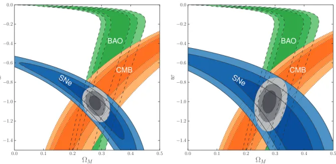
Under the bound (2.2.9), the density parameter is constrained to be 0.70 < ΩDE0 < 0.76. This is consistent with the bound coming from the SN Ia data. We can also show that, for increasing wDE, the observationally allowed values of Ωm0 gets larger. However, R depends weakly on the w^DE. Hence, the CMB data alone do not provide a tight constraint on wDE. In Fig. 2.3, we show the joint observational constraints on wDE and Ωm0 (for constant wDE) obtained from the WMAP 7-year data and the Union2 SN Ia data [90]. The joint observational constraints provide much tighter bounds compared to the individual constraint from CMB and SN Ia. For the flat universe, Amanullah

(28)

Figure 2.3: 68.3%, 95.4% and 99.7% confidence regions of the (ΩM0, w) plane from SN Ia combined with the constraints from BAO and CMB both without (left panel) and with (right panel) systematic errors. The flat universe (K = 0) and constant w have been assumed [90].

et al. [90] obtained the bounds wDE _{= −0.997}^+0.050−0.054^(stat)^+0.077−0.082(stat + sys together) and Ωm0 = 0.269^+0.019_−0.017(stat)^+0.023_−0.022(stat + sys together) from the combined data analysis of CMB and SN Ia.

2.2.3 Constraints from BAO

Eisenstein et al. [91] first reported the detection of Baryon Acoustic Oscillations (BAO) in a spectroscopic sample of 46, 748 luminous red galaxies observed by the “Sloan Digital Sky Survey” (SDSS). This has provided another test for probing the property of dark energy. Peaks and troughs in the angular power spectrum of CMB temperature anisotropies arise from gravity-driven acoustic oscillations of the coupled photon-baryon fluid in the early universe. After decoupling epoch, photons and baryons decouple and the sound speed of the baryons due to the loss of photon pressure. Sound waves remain imprinted in the baryon distribution and through gravitational interactions in the dark matter distribution as well. Since the sound horizon scale provides a standard ruler calibrated by CMB anisotropies, measurement of the BAO scale in the galaxy distribution provides a geometric probe of the expansion history. Since the impact of baryons on the far larger

(29)

dark matter component is small, in the galaxy power spectrum, this scale appears as a series of oscillations with amplitude of order 10%. This is more subtle than the acoustic oscillations in CMB.

The location of BAO is determined by the sound horizon at which baryons were released from the Compton drag of photons. This epoch (, called the drag epoch,) occurs at the redshift zd. The sound horizon at z = zdis given by rs(zd) =^∫₀^η^ddηcs(η). According to the fitting formula of z_d by Eisenstein and Hu [92], z_d and r_s(z_d) are constrained to be around zd≃ 1020 and r^s^(z^d) ≃ 150 Mpc.

We observe the angular and redshift distributions of galaxies as a power spectrum P (k⊥, k//) in the redshift space, where k⊥ and k// are the wavenumbers perpendicular and parallel to the direction of light respectively. In principle, we can measure the following two ratios [93]

θ_s(z) = ^r^s^(z^d⁾

d^(c)_A (z)^, ^(2.2.12)

δzs(z) = zs(zd)H(z), (2.2.13)

where the quantity θs(z) characterizes the angle orthogonal to the line of sight, whereas the quantity δzs corresponds to the oscillations along the line of sight.

The current BAO observations are not sufficient to measure both θs(z) and δzs(z) independently. From the spherically averaged spectrum, we can find a combined distance scale ratio given by [93]

(θ²_s(z)δzz(z)⁾^1/3_≡ ^r^s^(z^d⁾

{(1 + z)²^d²A(z)/H(z)}^1/3^, ^(2.2.14) or, alternatively, the effective distance ratio [91]

DV_{(z) ≡}

{ (1 + z)²d²_A(z)z H(z)

}1/3

. (2.2.15)

In 2005, Eisenstein et al. [91] obtained the constraint DV(z) = 1370 ± 64 Mpc at the redshift z = 0.35. In 2010, Percival et al. [94] measured the effective distance ratio

(30)

defined by

rBAO_{(z) ≡}

rs(zd)

DV(z)^, ^(2.2.16)

at the three redshifts: rBAO(z = 0.2) = 0.1905 ± 0.0061, r^BAO(z = 0.275) = 0.1390 ± 0.0037 and r_BAO(z = 0.35) = 0.1097 ± 0.0036. This is based on the data from SDSS Data Release 7 (DR7) and the 2-degree Field (2dF) Galaxy Redshift Survey. These data provide the observational contour of BAO plotted in Fig. 2.3. Amanullah et al. [90] placed the constraints wDE _{= −1.009}^+0.050_−0.054(stat)^+0.077_−0.082(sys + stat together) and Ωm0 = 0.277^+0.014_−0.014(stat)^+0.017_−0.016(sys + stat together) for the constant equation of state of dark energy in the flat universe from the joint data analysis of SN Ia [90], WMAP 7-year [71] and BAO data [94]. Hence, the ΛCDM model is well consistent with a number of independent observational data.

Finally, we should mention that there are other constraints coming from the cosmic age [95], large-scale clustering [96], gamma ray bursts [97] and weak lensing [98]. So far we have not found strong evidence for supporting dynamical dark energy models over the ΛCDM model, but future high-precision observations may break this degeneracy.

2.3 Cosmological constant

In 1917, Einstein originally introduced the cosmological constant Λ to achieve a static universe. After Hubble discovered the expansion of the universe in 1929, Λ was dropped by Einstein as it was no longer required. From the point of view of particle physics, however, the cosmological constant naturally arises as an energy density of the vacuum. If Λ originates from the vacuum energy density, the energy scale of it should be much larger than that of the present Hubble constant H0. Before the accelerated expansion of the universe is discovered [1, 2], this “cosmological constant problem” [3] was well known to exist long. There have been a number of efforts to solve this problem.

Attempts to evaluate the value of the energy density of the quantum vacuum lead to very large or divergent results. There is a zero-point energy ω/2 for each mode of a

(31)

quantum field with mass m, so that the vacuum energy density is given by

ρvac = ¹ 2

∑

fields

gi

∫ ∞ 0

d³k (2π)³

√k²+ m², (2.3.1)

where gi means the degrees of freedom of the field (the sign of gi is + for bosons and − for fermions) and the sum runs over all quantum fields, e.g., quarks, leptons, gauge fields, etc. This exhibits an ultraviolet divergence: ρvac _{∝ k}⁴. However, we expect that quantum field theory is valid up to some cut-off scale kmaxin which case the integral (2.3.1) is finite:

ρvac _≃

∑

fields

g_ik⁴_max

16π² ^. ^(2.3.2)

On the one hand, Λ is known as of order the present value of the Hubble constant H0

by observations, that is

Λ ≈ H0²

= (2.13h × 10⁻⁴² ^GeV⁾²^. ^(2.3.3)

This corresponds to the density of Λ

ρΛ = ^Λ 8πG

≈ 10⁻⁴⁷ ^GeV⁴^. ^(2.3.4)

On the other hand, if we take the cutoff to be the Planck scale (k_max = m_pl= 1.22 × 10¹⁹ GeV) where we expect the quantum field theory in a classical spacetime metric to break down, we find that the vacuum energy density is estimated as

ρvac _{≈ 10}⁷⁴ GeV⁴, (2.3.5)

which is about 10¹²¹ orders of magnitude larger than the observed value (2.3.4). It is very unlikely that a classical contribution to the vacuum energy density would cancel this quantum contribution to such high precision. Even if we take an energy scale of Quantum ChromoDynamics (QCD) for kmax, we obtain ρvac_{≈ 10}⁻³ GeV⁴ which is still much larger

(32)

than ρ_Λ. This very large discrepancy is known as the cosmological constant problem [3]. Supersymmetry (SUSY) which is the hypothetical symmetry between bosons and fermions, appears to provide a resolution of the zero-point energy. In SUSY theories, every fermion in the standard model of particle physics (SM) has an equal-mass SUSY bosonic partner that contributes to the zero point energy with an opposite sign compared to the fermionic degree of freedom, and vice versa. Therefore, fermionic and bosonic zero- point contributions to ρ_vacwould exactly cancel. However, none of the SUSY particles has yet been observed in collider experiments, so they must be sufficiently heavier than their SM partners. If SUSY is spontaneously broken at a mass scale M , we would expect the imperfect cancellations to generate a finite vacuum energy density ρvac _{∼ M}⁴. For a viable SUSY scenario, the SUSY breaking scale should be around M_SUSY ∼ 1 TeV because we want to ensure that no new scales are introduced between the electroweak scale (∼ 246 GeV) and the Planck scale. This also leads to a very large discrepancy from the observed value (2.3.4). We do not know how the Planck scale or SUSY breaking scales are really related to the observed vacuum scale.

(33)

Chapter 3 Alternative models to _{ΛCDM model}

3.1 Modified matter models

In this section, we shall briefly describe “modified matter models,” such as quintessence, K-essence, etc. In these models, the energy-momentum tensor T_µν on the right hand side of the Einstein equation contains an exotic matter source with a negative pressure. Scalar fields naturally arise in particle physics including string theory and these can act as candidates for dark energy. So far a wide variety of scalar-field dark energy models have been proposed. We have to keep in mind that the contribution of the dark matter component needs to be taken into account for a complete analysis. In this section, we shall study a flat FLRW universe (K = 0) unless otherwise specified.

3.1.1 Quintessence

A quintessence field [4, 5] is a scalar field with standard kinetic term, minimally coupled to gravity. The scalar field part action takes the form

S =

∫

d⁴x^√_−g [

−¹₂∇^µϕ∇^µϕ − V (ϕ) ]

, (3.1.1)

(34)

where V (ϕ) is the potential of the field. In the flat FLRW background, the variation of the action (3.1.1) with respect to ϕ gives

ϕ + 3H ˙¨ ϕ + ^dV

dϕ ^{= 0 .} ^(3.1.2)

Taking variation of g^µν, we obtain the stress-energy tensor:

Tµν _{= −}

√2

−g δS δg^µν

= ∇^µϕ∇^νϕ − g^µν^{[ 1}₂∇^λϕ∇^λ^{ϕ + V (ϕ)} ]

. (3.1.3)

The energy density and pressure can be derived from the stress-energy tensor as

ρ = −T⁰⁰

= ¹

2^ϕ^˙

2_{+ V (ϕ),} _(3.1.4)

P = Tⁱi

= ¹

2^ϕ^˙

2− V (ϕ) . ^(3.1.5)

Then, the Einstein equations becomes

H² = ^8πG 3

[ 1 2^ϕ^˙

2_{+ V (ϕ)}

]

, (3.1.6)

¨ a

a ^{= −}

8πG 3 ^{[ ˙ϕ}

2− V (ϕ)^] ^. ^(3.1.7)

The equation of state for the field ϕ is given by

wφ = ^P^φ ρφ

= ^ϕ^˙

2_{− 2V (ϕ)}

ϕ˙²+ 2V (ϕ)^. ^(3.1.8)

In order to answer what kind of potentials can give rise to acceleration of the present universe, we consider the power-law expansion

a(t) ∝ t^p^, ^(3.1.9)

(35)

where we have kept p general, keeping in mind that p = 1 corresponds to no acceleration and p > 1 corresponds to acceleration. From (3.1.6) and (3.1.7), we obtain the relation H = −4πG ˙ϕ˙ ². The field ϕ and the potential V (ϕ) can be solved from this relation as

ϕ =

∫ dt

[

−_4πG^H^˙ ]1/2

, (3.1.10)

V = ^3H

2

8πG (

1 + ^H^˙ 3H²

)

, (3.1.11)

where we chose the positive sign of ˙ϕ. Hence, The field and the potential driving the power-law expansion correspond to

ϕ ∝ ln t, ^(3.1.12)

V (ϕ) ∝ exp (

−^{√ 16π}_p _m^ϕ

pl

)

. (3.1.13)

Although the energy density for radiation (or matter) is much larger than that for the field ϕ during radiation-dominated (or matter-dominanted) era, the field energy density ρ_φ needs to dominate at present to be responsible for dark energy. From (2.1.24), the condition for the present cosmic acceleration corresponds to wφ < −1/3, i.e. ˙ϕ² ^{< V (ϕ)} from (3.1.8). This means that the potential for the scalar field needs to be flat enough for the field to evolve slowly. If the slowly rolling scalar field satisfying the condition

ϕ˙² _{≪ V (ϕ)} (3.1.14)

gives the dominant contribution to the energy density of the universe, we obtain the approximate relations

3H ˙ϕ + V,φ _{≃ 0} (3.1.15)

and

3H² _{≃ κ}²V (ϕ) (3.1.16)

from (3.1.2) and (3.1.6), respectively. Then, the equation of state for field in (3.1.8) is

(36)

approximately given by

wφ_{≃ −1 +}

2ϵs

3 ^, ^(3.1.17)

where ϵs ≡ {(dV/dϕ)/V }²^/(2κ²) is the so-called slow-roll parameter [72]. Since the potential is sufficiently flat, ϵ_s is much smaller than unity during the accelerated expansion of the universe. Note that the field equation of state deviates from −1 (w^φ> −1) unlike the cosmological constant.

3.1.2 K-essence

There are often scalar fields with non-canonical kinetic terms in particle physics. The scalar-field action for such theories is generally given by

S =

∫

d⁴x^√−gP (ϕ, X) , ^(3.1.18)

where P (ϕ, X) is a function of a scalar field ϕ and its kinetic energy

X ≡ −¹₂∇^µϕ∇^µ^ϕ. ^(3.1.19)

Quintessence relies on the field potential V (ϕ) to lead to the late-time accelerated expansion of the universe. Even in the absence of the potential energy of scalar fields, it is possible to realize the cosmic acceleration due to the kinetic energy X. Armendariz- Picon et al. [99] originally proposed kinetic energy driven inflation, called “k-inflation,” to explain inflation in the early universe. The application of these theories to dark energy was first carried out by Chiba et al. [6]. The analysis was extended to a more general Lagrangian by Armendariz-Picon et al. [7,8] and this scenario based on the action (3.1.18) was called “k-essence.” In these theories with the action (3.1.18), the pressure Pφ and the energy density ρφ of the field are

Pφ = P, (3.1.20)

ρφ = 2X^∂P

∂X ^{− P.} ^(3.1.21)

(37)

Then, the equation of state of k-essence is given by

wφ = ^P^φ ρφ

= ^P

2X∂P/∂X − P ^. ^(3.1.22)

As long as the condition |2XP^,X| ≪ |P | is satisfied, w^φ can be close to −1.

The action (3.1.18) includes a wide variety of theories, for example, the ‘ghost condensate model’ [100]. The theories with a negative kinetic energy −X generally suffer from the vacuum instability, but the presence of the quadratic term X² can avoid this problem. The model constructed in such context is the ghost condensate model whose Lagrangian is

P = −X + ^X

2

M⁴^, ^(3.1.23)

where M is a constant. In this model, we have

w_φ= ^{1 − X/M}

4

1 − 3X/M⁴ ^, ^(3.1.24)

which gives −1 < w^φ< −1/3 for 1/2 < X/M⁴ < 2/3. The de Sitter solution (wφ_{= −1),}

in particular, appears when X/M⁴ = 1/2. We can explain the present cosmic acceleration for M ≃ 10⁻³ eV because the energy density for the field is ρφ = M⁴/4 at the de Sitter point.

In order to discuss stability conditions of k-essence, we decompose the field into the homogeneous parts and perturbed parts as ϕ(t, x) = ϕ0(t) + δϕ(t, x) in the Minkowski background [101]. Then, the second-order Hamiltonian reads

δH =^{( dP} dX ^{+ 2X}

d²P dX²

) (δ ˙ϕ)²

2 ⁺

dP dX

(∇δϕ)²

2 ⁻

d²P dϕ²

(δϕ)²

2 ^. ^(3.1.25)

The term d²P/dϕ² is related with the effective mass of the field. From the positivity of

(38)

the first two terms in (3.1.25), we can derive the stability conditions: dP

dX ^{+ 2X} d²P

dX² ^{≥ 0,} ^(3.1.26)

dP

dX ^{≥ 0.} ^(3.1.27)

The propagation speed cs of the field is given by

c²_s = ^dP^φ^/dX dρφ/dX

= ^dP/dX

dP/dX + 2Xd²P/dX² ^, ^(3.1.28)

which is positive under the conditions (3.1.27). Furthermore, we also require the sound speed cs ≤ 1. This is satisfied when

d²P

dX² ^{> 0 .} ^(3.1.29)

3.2 Modified gravity theories

There is another class of dark energy models in which gravity is modified from general relativity. This class contains f (R) gravity, scalar-tensor theories, Gauss-Bonnet gravity, DGP braneworld model, etc. In this section, we will review “modified gravity theories.”

3.2.1 f (R) gravity

The simplest modification to general relativity is f (R) gravity with the action

S = ¹ 2κ²

∫

d⁴x^√_{−gf(R) +}

∫

d⁴_{x L}M, (3.2.1)

where f is a function of the Ricci scalar R and L^M is a matter Lagrangian for perfect fluids. The field equation can be derived by varying the action (3.2.1) with respect to gµν:

F (R)Rµν_{(g) −}

1

2^{f (R)g}^µν^{− ∇}^µ^∇^ν^{F (R) + g}^µν^{□F (R) = κ}

2_T

µν, (3.2.2)

本文 総合研究大学院大学学術情報リポジトリ 甲1589 本文

Cosmological tests of models for the accelerating

universe in terms of inhomogeneities

Keiki Saito

DOCTOR OF PHILOSOPHY

Department of Particle and Nuclear Physics

School of High Energy Accelerator Science

The Graduate University for Advanced Studies

2012

Contents

List of Figures

Chapter 1

Introduction

Chapter 2

Apparent accelerated expansion of

the present universe

2.1 FLRW cosmology

2.1.1 Isotropic and homogeneous universe

2.1.2 Kinematic properties of the expanding universe

2.2 Observational constraints on dark energy

2.2.1 Constraints from SN Ia

2.2.2 Constraints from CMB

2.2.3 Constraints from BAO

2.3 Cosmological constant

Chapter 3

Alternative models to ΛCDM model

3.1 Modified matter models

3.1.1 Quintessence

3.1.2 K-essence

3.2 Modified gravity theories

3.2.1 f (R) gravity

本文総合研究大学院大学学術情報リポジトリ甲1589 本文

Alternative models to _{ΛCDM model}