graph500 GPU HiPC2013

(1)

Parallel Distributed Breadth First Search on GPU

Koji Ueno

Tokyo Institute of Technology / JST CREST [email protected]

Toyotaro Suzumura Tokyo Institute of Technology IBM Research – Tokyo / JST CREST

Abstract— In this paper we propose a highly optimized parallel and distributed BFS on GPU for Graph500 benchmark. We evaluate the performance of our implementation using TSUBAME2.0 supercomputer. We achieve 317 GTEPS (billion traversed edges per second) with scale 35 (a large graph with 34.4 billion vertices and 550 billion edges) using 1366 nodes and 4096 GPUs. With this score, TSUBAME2.0 supercomputer is ranked fourth in the ranking list announced in June 2012. We analyze the performance of our implementation and the result shows that inter-node communication limits the performance of our GPU implementation. We also propose SIMD Variable-Length Quantity (VLQ) encoding for compression of communication data with GPU.

Keywords-component; GPU, BFS, Graph500, Supercomputer

I. ^INTRODUCTION

Graph500 [1] is a new benchmark for ranking supercomputers based on the performance of graph processing. Large graph analysis becomes more important in many fields such as social network analysis, electronic design automation and protein-protein interaction analysis. Since 1994, the best known de facto ranking of the world’s fastest computers is TOP500, which is based on a high performance Linpack benchmark for linear equations. As an alternative to Linpack, Graph500 was recently developed. Breadth First Search (BFS) is one of the core kernels of Graph500 benchmark.

Modern NVIDIA GPUs have very high peak computational performance. Utilizing GPUs requires many fine-grained parallel computations and regular memory access patterns. For dense matrix operations and image processing, exposing many fine-grained parallel computations and regular memory access patterns is easy. This enables these processors to achieve high percentages of peak floating point throughput and memory access bandwidth. However, a naïve parallel BFS algorithm is difficult to compute with fine-grained parallel computations, which SIMD GPU architecture requires for efficient processing. Also it has an irregular memory access pattern. Therefore, applying GPUs for graph processing has many difficulties.

In this paper, we propose an efficient parallel distributed BFS on GPU for Graph500 benchmark. We also analyze the performance and scalability of our implementation using the TSUBAME2.0 supercomputer. There are many papers for

optimizing BFS. However this is the first paper applying thousands of GPUs for large scale distributed BFS, as far as we know. We use our highly optimized algorithm for computing distributed BFS. Our algorithm uses 2D partitioning-based method that is scalable on large distributed memory systems, and our algorithm also uses many novel techniques such as vertex sorting for reducing memory access cost, compression of communication data, and sharing visited vertices for reducing communication data. We also use many GPU specific techniques for implementing BFS on GPUs.

Here are the main contributions of our paper:

1. We propose a highly optimized parallel and distributed BFS on GPU using many GPU specific techniques for optimization.

2. We propose new technique, SIMD Variable-Length Quantity encoding which enables compression and decompression of integer values using GPU with low computation cost.

3. We give a detailed analysis of our GPU implementation of BFS.

4. We show scalability of our GPU implementation using 4096 GPUs on the TSUBAME 2.0 supercomputer.

Here is the organization of our paper. In Section II, we give an overview of Graph500 benchmark, base algorithm and GPGPU. We review related work in Section III, In Section IV, we explain our highly optimized algorithm for distributed-memory BFS. In Section V, we describe the details of our GPU implementation of distributed memory based BFS. We give the performance evaluation of our method in Section VI and describe concluding remarks and future work in Section VII.

II. ^B^ACKGROUND

In this section, we give an overview of the Graph500 benchmark [1] and GPGPU.

A. Graph500 benchmark

In contrast to the computation-intensive benchmark used by TOP500, Graph500 is a data-intensive benchmark. It does breadth-first searches in undirected large graphs generated by a scalable data generator based on a Kronecker graph [2].

The benchmark has two kernels: Kernel 1 constructs an undirected graph from the graph generator in a format usable by Kernel 2. The first kernel transforms the edge tuples (pairs of start and end vertices) to efficient data structures

(2)

with sparse formats, such as CSR (Compressed Sparse Row) or CSC (Compressed Sparse Column). Then Kernel 2 does a breadth-first search of the graph from a randomly chosen source vertex in the graph and creates a BFS tree.

The benchmark uses the elapsed times for both kernels, but the rankings for Graph500 are determined by how large the problem is and by the throughput in TEPS (Traversed Edges Per Second). This means that the ranking results basically depend on the time consumed by the second kernel.

After both kernels have finished, there is a validation phase to check if the result is correct. The validation phase uses 5 validation rules to check correctness of the result. For example, the first rule is that the BFS graph is a tree and does not contain any cycles.

The problem size is defined by a Scale parameter, which is the base 2 logarithm of the number of vertices. For example, the Scale 26 means 2²⁶ vertices and corresponds to 10¹⁰ bytes occupying 17 GB of memory.

Vertices Degree

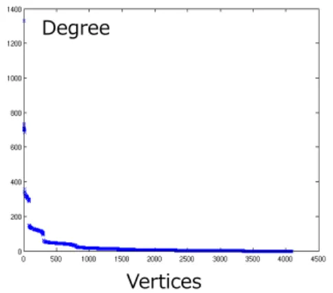
Figure 1. Degree Distribution of the Kronecker Graph used by Graph500

The Kronecker graph used by Graph500 benchmark has a skewed degree distribution. Figure 1 shows the degree distribution of the generated graph which has 4,096 vertices. The x-axis is the vertex ID sorted by degree and the y-axis is the degree (# of vertices). As shown in the graph, most of the vertices have low degrees and a small number of vertices have high degrees. The highest degree is more than 1,200. B. GPGPU (General Purpose computing on GPU)

Applying GPUs, which are graphics processing units, to general purpose computing has become popular recently due to their relatively low cost and high performance. Modern NVIDIA GPUs have tens of processor cores and each processor core uses SIMD. In CUDA, which is the programming framework provided by NVIDIA, each SIMD lane is represented as a thread. A single SIMD instruction executes instructions of each thread in a group called a warp. A thread block is a group of threads that will be co-located on the same processor core and share a local scratch memory called shared memory. Threads in a group of thread blocks execute a single program that is called a kernel. A sequence of kernels is executed in a bulk-synchronous manner.

III. R^ELATED^W^ORK

In this section, we give an overview of related work. Because large-scale graph analysis is a hot topic, there are many papers related to optimizing the performance of BFS. A. BFS on Distributed Memory Systems

Yoo et al. [5] propose a 2D partitioning of adjacency matrix, which is scalable on large distributed memory systems and they present the performance of their implementation on BlueGene/L with 32,768 nodes. Our paper uses an optimized algorithm based on their 2D partitioning method.

Buluç and Madduri [6] compare the performance of 1D partitioning method and 2D partitioning method using two supercomputers, `Hopper', a 6392-node Cray XE6 and

`Franklin', a 9660-node Cray XT4.

Satish et al. [20] proposed an efficient distributed BFS for Intel CPU and Infiniband network supercomputers. Checconi et al. [21] proposed an efficient distributed BFS for BlueGene supercomputers. Both these two papers proposed novel algorithms that can reduce communication volumes dramatically. Reducing communication volumes is important for distributed BFS. The base ideas of reducing communication volumes on these two papers seem to be similar. Our approach for reducing communication volumes is partially the same as theirs but we have our own ideas such as SIMD VLQ.

B. BFS on GPUs

It is not easy to implement an efficient BFS algorithm on GPUs. Harish et al. [7] and Hussein et al. [8] implemented a simple and suboptimal algorithm on GPUs. Their algorithm inspects every vertex during every iteration.

Luo et al. [9] proposed a hierarchical queue structure to maintain a global queue on the GPU. Instead of inspecting every vertex, their algorithm inspects the vertices contained in the queue which is equivalent to CQ in the Algorithm I. Their algorithm is more efficient than the prior work. However their algorithm is not efficient for the graphs that have skewed degree distribution like Kronecker graphs.

Hong et al. [10] proposed warp based processing method on GPUs. Rather than threads, warps are used to read edge lists. With their method, GPU implementation can efficiently process the graphs that have skewed degree distribution. They improved their method [11] to use a queue instead of inspecting every vertex, when the number of vertices in NQ is small.

Merrill et al. [12] described highly optimized BFS implementation on the GPU. They proposed a novel dynamic scheduling technique on the GPU, which solves load imbalance from edge list expansion and enables efficient processing for any type of real world graphs. But their algorithm is optimized for a single node and can only handle several GPUs at maximum. Our GPU implementation uses their technique for edge list expansion.

C. BFS on Other Architectures

Agarwal et al. [2] proposed an efficient BFS algorithm for commodity multicore processors such as the 8-core Intel

(3)

Nehalem EX processor. They proposed a bitmap technique for reducing the amount of working memory. This technique is commonly used by many implementations including our GPU implementation.

Bader and Madduri [4] described the performance of parallel BFS algorithms on multithreaded architectures such as the Cray MTA-2. Scarpazza et al. [13] implement BFS on Cell/BE processor.

IV. P^ARALLEL^BFS^A^LGORITHM In this section, we describe parallel BFS algorithms. A. Level-synchronized Parallel BFS

Most parallel BFS algorithm use a “level-synchronized parallel breadth-first search”, which means that all of the vertices at a given level of the BFS tree will be processed (potentially in parallel) before any vertices from a lower level in the tree are processed. The details of the level- synchronized BFS are explained in [3][4]. Let V and E is the vertex and edge sets of the graph and n is the number of vertices in V, m is the number of edges in E.

Algorithm I: Level-synchronized Parallel BFS Input: r is the source vertex of BFS.

Output: PRED has predecessor vertices for each vertex and forms a BFS tree.

Algorithm I is the abstract pseudocode for the algorithm that implements level-synchronized parallel BFS. Each processor has two queues, CQ and NQ, and two arrays, PRED for a predecessor array and VISITED to track whether or not each vertex has been visited. In many optimized implementations, VISITED is implemented as a bitmap, each bit of which represents whether the corresponding vertex is visited or not.

At any given time, CQ (Current Queue) is the set of vertices that must be visited at the current level. At level 1, CQ will contain the neighbors of r, which is a source vertex of BFS, so at level 2, it will contain the pending neighbors (the neighboring vertices that have not been visited at levels 0 or 1). The algorithm also maintains NQ (Next Queue), containing the vertices that should be visited at the next level. We use the term, edge frontier, for the set of all edges to be traversed during that level. In other words, edge frontier is

the set of all edges emanating from the vertices contained in CQ.

PRED has predecessor vertices for each vertex. If an unvisited vertex v is found at line 12, the vertex u is the predecessor vertex of the vertex v at line 14. When we complete BFS, PRED forms a BFS tree, the output of kernel 2 in the Graph500 benchmark.

B. 2D Partitioning of Adjacency Matrix

We found that the 1D partitioning method is not scalable in [14]. For a scalable distributed parallel breadth-first search, a 2D partitioning of the adjacency matrix was proposed in [5]. Their scalable approach uses a level-synchronized parallel BFS and 2D partitioning method to reduce the communication costs. Our algorithm optimizes this 2D partitioning method and also uses further optimization techniques. Here is a brief overview of the 2D partitioning method.

Figure 2. 2D partitioning of adjacency matrix [5]

Assume that we have a total of P processors, where the C

R

P_ _ processors are logically deployed in a two dimensional mesh which has Rrows and C columns. We use the terms processor-row and processor-column with respect to this processor mesh. Adjacency matrix is divided as shown in Figure 2 and the processor ( ji, ) is responsible for handling the C blocks from A_i⁽_{, j}¹⁾ to A_i⁽_,^C_j⁾. In Figure 2, we assume that the edge list for a given vertex is a column of the adjacency matrix. Therefore, each edge list is divided and each block has partial edge lists. The vertices are divided into R_C blocks and the processor ( ji, ) handles the k-th block, where k is computed as (j_{ )}1_R_i.

Each level of the level-synchronized parallel BFS method with 2D partitioning is done in 2 communication phases called “expand” and “fold”. Before the expand phase, each processor has its own NQ, which contains the NQ vertices owned by that processor. Assume that NQ contains the vertex v. The processors in the same processor-column of the owner of v may have a partial edge list. Thus these processors need to know the vertex v. Therefore, in the expand phase, every processor sends its NQ to all of the

(4)

other processors in the same processor-column and the received NQ becomes CQ. Then the edge lists of the vertices in CQ are merged to form a set of edge frontier. In the fold phase, each processor sends the edges of the edge frontier to the owner of their destination vertices. With the 2D partitioning, these owners are in the same processor-row.

The advantage of 2D partitioning is to reduce the number of processors that need to communicate. 1D partitioning requires all-to-all communication. However, with the 2D partitioning, each processor only communicates with the processors in the processor-row and the processor-column.

The algorithm of 2D partitioning method is shown in Algorithm II. We use bitmaps for CQ, NQ and VISITED. Each bit of CQ (NQ) bitmap represents whether the corresponding vertex is contained in CQ (NQ) or not. Each bit of the VISITED bitmap represents whether the corresponding vertex is already visited or not. The length of the CQ bitmap, NQ bitmap and VISITED bitmap is n/C, n/P and n/P respectively.

In the fold phase, we do not have to send all the edges in the edge frontier. If a processor receives multiple frontier edges that have the same destination, this processor only needs one edge within these edges and the other edges will not be used. Therefore, a sender processor can reduce multiple frontier edges that have the same destination. This reduction operation, which we call reducing edge frontier, is important to reduce the communication data volume of the fold phase. [5] and [6] reduce the edge frontier in different ways.

Algorithm II: Distributed BFS with 2D partitioning Input: r is the source vertex of BFS.

Output: PRED has predecessor vertices for each vertex and forms a BFS tree.

1 for all vertices v do 2 | PRED[v]← -1; 3 | VISITED [v] ← 0; 4 PRED [r] ← 0; 5 VISITED[r] ← 1; 6 Enqueue(NQ, r); 7 fork;

8 for level = 1 to

_

9 | CQ ^← all gather NQ in this processor-column; (expand) 10 | NQ ←_;

11 | for all u in CQ do 12 | | u ← Dequeue(CQ);

V. ^GPU^IMPLEMENTATION

In this section, we give an overview of our algorithm and its GPU implementation and then describe the details of our method.

A. Algorithm Overview

We use a 2D partitioning method. The communication pattern and distribution of data such as NQ, CQ and adjacency matrix are exactly the same as the method described Section IV-B. We mapped a processor of a 2D partitioning method to a single GPU. We need CPU resources for communication between GPUs and some portion of computation. The compute node of TSUBAME2.0, we used for performance evaluation, has 3 GPUs and 2 CPU sockets, 24 CPU threads in total. We assigned 8 CPU threads to each GPU.

2. Compression and communication of expand phase

3. Decompression of expand phase 1. Communication of expand using

bitmap

4. Generating CQ list

5. Gathering edges

6. Filtering edges

7. Compression and communication of edge frontier

8. Status lookup and updating NQ

Yes ^No

In parallel

Receiver processing Sender processing

Level start

Level end

Processing on CPU Processing on GPU If # of Vertices in NQ is larger than

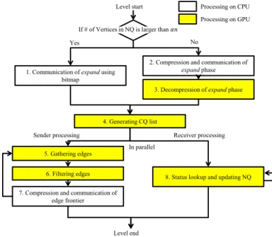
Figure 3. Computational flow of one level at the level synchronized BFS on GPU

Figure 3 illustrates the computational flow of one level of the level-synchronized BFS on each processor. We were able to implement most of the processing on the GPU, but since some portions of the code could not be executed efficiently on GPUs, we implemented those parts on the CPU. The number in Figure 3 is just a label and is not the order of processing.

The task 1-3 are the communication of the expand phase, which correspond to line 9 of Algorithm II. NQ is represented by a bitmap, and the bitmap can be used for communication, but if the number of vertices in NQ is small, the data becomes redundant which leads to low efficiency. Therefore, we dynamically select the data representation of this communication. The parameter  is a threshold of selecting data representation. If the total number of vertices in NQ is more than _ n, where n is the number of vertices in the graph, we use bitmap for communication. If it is not, we use a compressed vertex list, which is described in the next section. We used 1/16 for the parameter.

(5)

Tasks 4-7 correspond to line 11-14 of Algorithm II. Task 4, Generating CQ list, is the process of listing up the word - within the CQ bitmap where at least one bit is set (we call this “non-empty word” and NW hereafter). A word is a data type that can be efficiently processed by GPUs. The current version of CUDA adopts 32 bits. The CQ bitmap can be used directly for further processing, but if the number of NW is small in the CQ bitmap, load imbalance may occur when processing this with GPUs. Therefore, it is better to retrieve only NWs and list them up. Task 5, Gathering edges, creates the edge frontier, the set of all edges emanating from the vertices contained in CQ, from the CQ list and adjacency matrix. Task 6, Filtering edges, reduces edge frontier. Section V-E describes this method. The implementation of this process is simple. It just checks a bitmap for the destination vertex of the edge.

Task 8 corresponds to line 15-19 of Algorithm II. This task receives a compressed edge frontier, transfers the received data to the GPU without any processing on CPU and all tasks are processed on the GPU.

We parallelized tasks 5-7 (sender processing) and task 8 (receiver processing). The CQ list within a single GPU is divided into several parts and processed in different kernel launches. The communication of the edge frontier will start immediately after the corresponding portion of the CQ list is processed. The received edge frontier is buffered and task 8 will start immediately after the size of the buffered edge frontier exceeds a threshold. This enables the overlapping communication with computation, which also reduces the working memory size. If we process all tasks 5-7 before starting task 8, all the edges that will be transferred to the other processors have to be stored on memory temporarily. This prevents the overlapping communication with computation and increases working memory size.

B. Expand Compression

The expand phase creates CQ by exchanging NQ with C processors in the processor-column. Our prior work [14] exchanges NQ by using the bitmap. However, if the number of vertices in NQ is small, the data becomes redundant which leads to low efficiency. Thus we propose the method of dynamically selecting the data representation depending on the number of vertices in NQ, whether it is a bitmap or a list of compressed vertices. This method reduces the communication data volume in the expand phase.

The compressed vertex list is generated by sorting out the vertices to be transmitted in a decreasing order of vertex id, computing the difference of the anteroposterior vertices id, and then compressing it with base 128 variable-length quantity encoding which is used by the standard MIDI file format and Google’s protocol buffers etc. We use general variable-length quantity (VLQ) for unsigned integers. In this encoding, an integer value will be one or more bytes. Smaller numbers will be smaller number of bytes. The most significant bit (MSB) of each byte indicates whether another VLQ byte follows. If the MSB is 1, another VLQ byte follows and if 0, this is the last byte of the integer. The remaining 7 bits of each byte form an integer. The least significant bit will be first in a stream. Because VLQ is byte-

aligned coding, it is faster than bit-level coding such as Rice coding and Huffman coding. The data volume per vertex can be compressed to 1 byte at minimum. If the number of vertices in NQ is more than 1/8 of all the vertices, the bitmap as data representation becomes smaller. However if it is less than 1/8, the compressed vertex list could become smaller.

However, the method of employing the compressed vertex list needs the compression and decompression, and de-serializing the bitmap information after the communication. Thus if the data size of the compressed vertex list and bitmap are the same, it is efficient to conduct the communication with the bitmap information. We use the parameter, a threshold of selecting the data representation. If the total number of vertices in NQ is more than _n, where n is the number of vertices in the graph, we use the bitmap for communication. If it is not, we use the compressed vertex list. We choose 1/16 for parameter_ . Algorithm III shows the pseudocode for this process.

Algorithm III: Compressed Expand Communication Input: NQ.

Output: CQ

 is a threshold of selecting data representation of expand. n is the number of vertices in the graph.

1 fv ^← all reduce |NQ|; // compute the number of vertices in NQ 2 if fv > __nthen // expand using bitmap

3 | CQ ^← all gather NQ in this processor-column; 4 else // expand using compressed vertex list 5 | NQlist ^← compress NQ;

6 | CQlist ^← all gather NQlist in this processor-column; 7 | CQ ^← decompress CQlist;

C. SIMD Variable-length Quantity Encoding

The compression method described in the previous section uses VLQ encoding to compress the communication data. But the original VLQ encoding cannot be processed in parallel. We propose a “SIMD VLQ Encoding” method to efficiently process the encoding with GPUs in this paper.

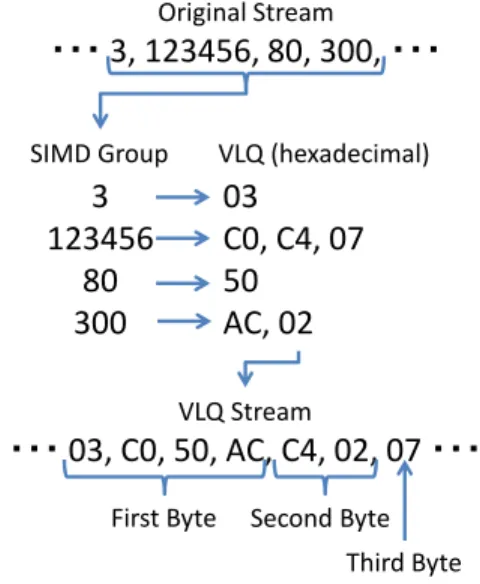
SIMD VLQ Encoding is optimized by considering the SIMD width of GPUs, where the order of VLQ bytes is changed. The original VLQ Encoding allocates each VLQ byte of a single value in a contiguous fashion, whereas the SIMD VLQ Encoding method groups values by the SIMD width and each byte of VLQs is allocated in a following fashion. The first byte of each VLQ is contiguously allocated and the second byte, the third byte etc. is done in the same way. If there are no more bytes in the VLQ, the space for that VLQ is not allocated. Figure 4 shows the encoding example by SIMD VLQ Encoding in a case where the SIMD width is 4. In the figure, the sequence of “3,123456,80,300” is compressed into “03,C0,50,AC,C4,02,07”. The original sequence consumes 16 bytes if each value is represented by 4 byte values. The compressed sequence consumes only 7 bytes. For simplicity, this example in the figure employs a small SIMD width, but it is 32 in the case of CUDA. Algorithm IV is a code example of the decoding by CUDA. This figure only illustrates the decoding, but the encoding is also processed in the same manner.

(6)

VLQ Stream

・・・ 03, C0, 50, AC, C4, 02, 07 ^・・・

3 123456

80

300

Original Stream

・・・ 3, 123456, 80, 300, ^・・・

SIMD Group VLQ (hexadecimal)

03 C0, C4, 07

50 AC, 02

First Byte Second Byte Third Byte Figure 4. SIMD VLQ encoding example (SIMD width is 4)

Algorithm IV: SIMD VLQ Decoding with CUDA Input: VLQ stream VLQs, length for the number of values to be decoded

Output: , decoded stream s, VLQ stream length VLQ_length Functions: __popc counts the number of set bits of input value. __ballot is CUDA specific function.

1 volatile shared s_offset ; 2 mask = (1 << thread_id) - 1; 3 v = 0; offset = 0; s_offset = 0;

4 for(i = thread_id; i < length; i += WARP_SIZE) { 5 | for(j = 0; ; j += 7) {

6 | | flags = __ballot(1);

10 | | offset += __popc(flags); 11 | | s_offset = offset; 12 | | if(v < 0x80) break; 13 | }

14 | s[i] = v; 15 | offset = s_offset; 16 }

17 VLQ_length = s_offset;

There are similar techniques. Balevic [18] proposed parallel Variable Length Encoding (VLE) for GPUs. However, their target is VLE using Huffman coding. VLE is a similar but different technique than VLQ. Since they try to parallelize VLE without reordering the compressed stream data, they have to use prefix sum and atomic operations. The compression rate of VLQ is smaller than the Huffman coding but SIMD VLQ is faster than their method. Google proposed Group Varint Encoding [19] for faster processing of VLQ Encoding. However, they focused on CPU processing and not on GPU. Since the SIMD width of GPUs is relatively larger than that of CPUs, we cannot apply their method on GPUs.

Our SIMD VLQ can process both encoding and decoding on GPUs. SIMD VLQ can be used not only for our BFS method but also many applications that need fast VLQ encoding.

D. Generating CQ list

Generating the CQ list is the process of listing up the non-empty words. The CQ bitmap can be used directly for further processing, but if the number of NW is small in the CQ bitmap, load imbalance may occur when processing this on GPUs. Therefore, it is better to retrieve only NWs and list them up. Our GPU implementation computes the offset of NWs with a prefix sum after counting the NWs. Merril [15] describes several efficient prefix scan methods. We used a combination of his methods, which is two-level streaming reduce-then scan, two way conflict Brent-Kung parallel scan, and SIMD Kogge-Stone parallel scan. All these methods are explained in [15].

E. Gathering Edges

Gathering edges creates the edge frontier from the CQ list and adjacency matrix. If this process is implemented in a straightforward manner, load imbalance among GPU threads would become problematic. However, Merril [12] proposed the solution for this load imbalance problem by what they call “Scan+warp+CTA gathering” (CTA is the same as thread block in CUDA). Gathering edges needs the buffer for storing the gathered edges, but it is difficult to predict the necessary size of the buffer. Moreover, since the GPU memory size is limited, it is difficult to dynamically allocate the required memory during the kernel execution. Therefore, our implementation terminates the GPU kernel for gathering edges once the buffer is filled out, and afterward it again conducts the edge gathering processing for the remaining portion.

We intended to implement tasks 5-6, Gathering edge and Filtering edge, into a single CUDA kernel since dividing them into two kernels increases the memory access. If we implement task 5-6 by a separate kernel for each task, all the gathered edges have to be stored into memory and then read by the next kernel. If we can implement both tasks with a single kernel, gathered edges are processed at the same time and we need not store the edges to memory. Since the data size of the graph edges is large, we want to reduce the cost of writing/reading the edge data into/from memory. However, the single composed CUDA kernel requires a large amount of GPU registers, which leads to low efficiency. We compared the two methods and decided to choose dividing into two kernels since it has better performance than the single composed kernel.

F. Filtering edges

As mentioned in the Section IV-B, reducing the edge frontier is important to scalable distributed BFS. The edge frontier can be reduced before sending it to the owner processor of its destination vertex, and reducing the edge frontier is important to reduce the communication data volume of the fold phase.

Our prior work [14] does not reduce the edge frontier. Instead, our prior algorithm compresses the communication data. We are able to compress the data with low computation cost, but the communication data is relatively large even if it is compressed. Therefore the performance of our prior algorithm is limited by the communication cost.

(7)

1) Using Bitmap for Reducing Edge Frontier

In our new method, each processor has a bitmap whose each bit represents whether the destination vertex is visited or not. When we send the frontier edge, we mark the destination vertex of the frontier edge as visited. Before sending the frontier edge, we check whether the destination vertex is marked as visited in this bitmap and if it is marked we do not send that edge. We call this bitmap Shared Visited (SV). Satish et al. [20] also use the similar method to reduce the communication data volumes. With the 2D partitioning method, the length of SV is n/R bits. SV is different from VISITED of the Algorithm II. SV is the visited bitmap on the sender side for reducing frontier edge. VISITED of the Algorithm II is the visited bitmap on the receiver side, which avoids duplicate vertices from being queued into NQ.

2) Sharing Visited Vertices in the Same Processor- column

In the original 2D partitioning method, the expand phase sends NQ to the same processor-row. We propose the shared visited vertices technique for further optimization. In this technique, the expand phase sends NQ to the same processor-column as well as the same processor-row. After receiving NQ from other processors in the same processor- column, a processor updates the SV so that the vertices in NQ are marked as visited. Since the vertices in NQ are the vertices already visited, the processor does not need to send the frontier edge whose destination belongs to NQ. Therefore we mark NQ vertices as visited. This technique can further reduce the edge frontier.

3) Implementation Detail

Filtering edges reduces the edge frontier by checking the SV bitmap. Algorithm V shows the pseudo code for this process. In this process, the random access to SV is required and it is important to optimize this memory access.

Algorithm V: Checking SV (shared visited) Description: checking the bit corresponding to the vertex v and updating it.

Input: w_idx is the word index that has the bit corresponding to v. mask is a word. In mask, one bit which corresponding to v is set.

Output: s is whether v is visited or not. (A) “test-and-set”

1 s = !(atomicOr(&SV[w_idx], mask) & mask) ; (B) “test and test-and-set”

1 s = 0

2 if(SV[w_idx] & mask) == 0)

3 | s = !(atomicOr(&SV[w_idx] , mask) & mask); (C) “test and set”

1 s = 0

2 if(SV[w_idx] & mask) == 0) { 3 | SV[w_idx] = SV[w_idx] | mask; 4 | s = 1;

5 }

First, we implemented the straightforward method illustrated in Algorithm V (A), which executes read and write with one single atomic operation. We call (A) “test- and-set”. We also implemented the optimized version, (B) and (C) that reduces the number of the atomic operations. The method (B) obtains the same computational result as (A).

We call (B) “test and test-and-set”. The method (C) does not use any atomic operations. We call (C) “test and set”. With the (C) method, the update by some threads becomes invalid because SV cannot be updated in an atomic fashion in the case that more than 2 threads simultaneously update the same word.

G. Consideration on Performance Efficiency

Distributed BFS on GPUs has many difficulties that cause performance degradation in comparison to the single node case. In this subsection, we describe this topic.

When the problem size is larger than Scale 32, a 32 bit integer cannot represent the vertex id. We must use 64 bit integer for these large graphs. But current NVIDIA GPUs do not support 64 bit integer natively. A 64 bit integer is stored into two 32 bit registers and a 64 bit arithmetic operation is divided into multiple instructions, which degrades the performance. In our implementation, one edge is represented as 48 bit integer consisting of one 32 bit integer and one 16 bit integer. Reading one edge is divided into two memory operations. We also use many shift operations on 64 bit integer for computing owner processor of edges, local index of vertices and word index of bitmaps etc. Thus, our implementation requires 64 bit integers.

In addition to the above problem, inter GPU communication cost is large because a single inter GPU communication needs three steps, transferring from GPU memory to CPU memory, inter-node communication and transferring from CPU memory to GPU memory. Moreover, distributed BFS algorithm is more complex than single node algorithm. For example, our implementation uses 2D partitioning method, which needs two phase communication and computation whereas single node BFS can be implemented using only one phase. We need two steps of status lookup, SV and VISITED, for reducing communication data whereas single node BFS only needs VISITED. The efficiency of our GPU implementation of a distributed BFS will be much lower than the implementations of a single node BFS [11] [12].

VI. PERFORMANCE EVALUATION

We used TSUBAME 2.0 [16], the 21st fastest supercomputer in the TOP500 list of June 2013, to evaluate the performance of our GPU implementation.

A. Overview of the TSUBAME 2.0 supercomputer

TSUBAME 2.0 is a production supercomputer placed at the Tokyo Institute of Technology. TSUBAME 2.0 has more than 1,400 compute nodes interconnected by Infiniband network. Each TSUBAME 2.0 node has two Intel Westmere EP 2.93 GHz processors (Xeon X5670, 256-KB L2 cache, 12-MB L3), three NVIDIA Fermi M2050 GPUs, and 50 GB of local CPU memory. Each M2050 GPU has 2.8 GB of memory. Each of the CPUs in TSUBAME 2.0 has six physical cores and supports up to 12 hardware threads with Intel’s hyper-threading technology. Each node is interconnected by two links of QDR Infiniband. The total bandwidth is 8GB/s per direction. TSUBAME 2.0 uses a full-bisection fat-tree topology.

(8)

B. SIMD Valiable-length Quantity Encoding

In this subsection, we give the performance evaluation of SIMD VLQ encoding, which we explained in the section V- B. We measure the speed of encoding and decoding the sequence which has uniform random values from 0 to N. Figure 5 is the comparison the speed of a single GPU and a sequential CPU implementation which uses simple VLQ encoding. The x-axis is the number N and the y-axis is log scale of the throughput, million values per second. Since the CPU implementation suffers branch prediction misses, the values of the sequence to be processed highly affect the performance of the CPU implementation. The GPU implementation, which uses SIMD VLQ encoding, is 11-25 times faster than sequential CPU implementation. This result shows that our SIMD VLQ method can fully utilize the GPU performance.

C. Evaluation Method

Next, we analyzed the overall performance of our GPU implementation of BFS. In the software environment we used gcc 4.3.4 (OpenMP 2.5) and MVAPICH2 [17] version 1.6 with a maximum of 1366 nodes and CUDA version 4.1. The CPU side of our GPU implementation uses a hybrid of OpenMP and MPI. Each MPI process hosts a single GPU, which corresponds to a processor of the 2D partitioning method. We used MPI allgather(v) for the expand phase communication. We used MPI isend/irecv for the fold phase communication to realize the overlapping communication.

The 2D-partitioning processor allocation R_C is shown in Table 1. R and C are determined under the policy of allocating denominators as similarly as possible. The number of MPI processes should be a power of two and the value of R and C was determined by the MPI processes irrespective of the number of nodes.

Table 1. The values of R and C with the # of MPI processes

# of MPI processes 64 128 256 512 1024 2048

R 8 8 16 16 32 32

C 8 16 16 32 32 64

The graph data we used is a Kronecker graph with the initiator parameters (A,B,C) = (0.57,0.19,0.19), which is used in the Graph500. Since we mainly focus on the Graph500, we only test this graph. Edge factor, the ratio of the graph's edge count to its vertex count, is 16, which means the average degree of a vertex in the graph is 32.

Table 2. The performance of our GPU implementation submitted to the Graph500 June 2012. (Scale 35, 64 execution with 4096 GPUs)

GTEPS GTEPS

Minimum 74.9 First quartile 300 Median 317 Third quartile 326 Maximum 334

The result in this paper is the median of 16 BFS executions. We show only the median but the performance difference on each execution is relatively small. Table 2 shows the performance we submitted to the Graph500 June 2012. Since each GPU has 2.8 GB of memory, the maximum problem size we can solve on GPU memory is Scale 23 per GPU. We use this problem size for performance evaluation.

D. Effect of Optimization

Figure 6 and 7 show the effect of the expand compression with SIMV VLQ encoding, described in the Section V-B and V-C. Base performance is measured when all expand communication is performed using bitmap. Optimized implementation dynamically selects the data representation. Both Figure 6 and 7 are measured by executing a full distributed BFS. The graph data size is determined by a weak scaling fashion. Figure 6 shows the total execution time of the expand phase and Figure 7 shows communication data size of the expand phase per GPU.

The result shows that expand compression can reduce both communication data size and execution time of the expand phase dramatically.

Figure 8 shows the execution time of filtering kernel in three updating SV methods. The execution time of (B) and (C) is much less than that of (A). This result indicates that

“test and test-and-set” method, which is proposed in [3] and effective on the CPU, is also effective on the GPU. Figure 8 also shows that there is no difference between (B) and (C).

We expected that (C) would be faster than (B) because (C) does not use atomic operations but the result is that there is no difference. It seems that the atomic operations on the cached memory address are very fast on the modern NVIDIA GPUs.

Figure 9 shows the overall performance of our GPU implementation and also shows the effect of optimizations such as the expand compression and updating SV without atomic operation. The problem size is in a weak-scaling setting and Scale 23 per GPU. The unit of y-axis is GTEPS (billion edges per second). In Figure 9, Base is the performance of the base implementation, which communicates every expand phase with a bitmap and updates SV with the method (A) of Algorithm V. Expand compression improves the performance up to 25%. The method (B) or (C) of Algorithm V further improves the performance up to 58%.

We use expand compression and the method (B) of Algorithm V for subsequent performance evaluations. E. Profiling Execution Time and Communication Data

Size

Figure 10 is the breakdown of overall execution time. There is little difference on the total GPU kernel execution time. But as the number of GPUs increases, wait time, which is the sum of CPU processing time and communication wait time, becomes larger.

Since CPU computation of our GPU implementation is very small, most of wait time is communication wait time. Our implementation utilizes the overlapping communication with computation except the expand communication. This result shows that the performance bottleneck of our GPU implementation is the network communication bandwidth. In case of 4096 GPUs, 58% of the total execution time is spent to network communication.

Figure 11 shows communication data size of each expand phase and fold phase. Figure 12 shows the size of data transferred between CPU and GPU, which increases proportionally to the communication data size. As the

(9)

number of GPUs increases, the communication data size of both the expand phase and fold phases becomes larger. In the case of the expand phase, communication data size will be larger in proportion to R and C because the communication type at the expand phase is a broadcast operation within the processor-column and processor-row. In the case of the fold phase, if C becomes larger, there are more copies of SV. More copies of SV weaken the effect of reducing edge

frontier. Thus communication data increases. Large communication data increases the time of BFS and degrades the performance.

The ratio of kernel execution time to total elapsed time using 256 GPUs is 71 %, which demonstrates relatively high efficiency, but when using 4096 GPUs it is only 42%. If we can remove the communication bandwidth limit, the performance of our implementation will be double in the 100

200 400 800 1600 3200 6400 12800

1.E+02 1.E+03 1.E+04 1.E+05 1.E+06 1.E+07 1.E+08 Throughput (million values per second)

N

Encode (CPU) Decode (CPU) Encode (GPU) Decode (GPU)

Figure 5. Performance of SIMD VLQ encoding. Comparison with sequential CPU implementation

0 100 200 300 400 500 600 700 800 900

256 512 1024 2048

Time of expand phase (ms)

# of GPUs Base Expand Compression

Figure 6. Effect of expand compression.

0 100 200 300 400 500 600 700 800 900

256 512 1024 2048

Aggregated Message Size of Expand Phase per GPU (MB)

# of GPUs Base Expand Compression

Figure 7. Effect of expand compression.

0 200 400 600 800 1000 1200

256 512 1024 2048

Time of filtering edges kernel (ms)

# of GPUs test-and-set

test and test-and-set test and set

Figure 8. Comparison of updating SV methods.

0 50 100 150 200 250

0 500 1000 1500 2000 2500

GTEPS

# of GPUs base

Expand Compression

Expand Compression, "test and test-and-set" Expand Compression, "test and set"

Figure 9. Effect of optimization. (Weak scaling, Scale 23 per GPU)

0 200 400 600 800 1000 1200 1400 1600 1800

256 512 1024 2048 4096

Elapsed Time (ms)

# of GPUs fold wait time expand wait time time of expand kernel

time of receiver processing kernel time of filtering edges kernel time of gathering edges kernel time of generating CQ list kernel

Figure 10. Performance breakdown of the overall execution times. (Weak scaling, Scale 23 per GPU)

0 50 100 150 200 250 300 350

256 512 1024 2048 4096

Aggregated Message Size per GPU (MB)

# of GPUs fold

expand

Figure 11. Communication data size per GPU.

0 100 200 300 400 500 600 700 800 900

256 512 1024 2048 4096

Amount of data transfered per GPU (MB)

# of GPUs

Figure 12. Data size transferred between a CPU and a GPU.

0 50 100 150 200 250 300 350

0 500 1000 1500

GTEPS

# of nodes 3GPU/node 2GPU/node CPU

Figure 13. Comparison with CPU implementation.

(10)

case of using 4096 GPUs. Furthermore, we can increase the performance by further reducing the communication data volumes.

F. Comparison with CPU implementation

Figure 13 shows the performance of using 3 GPUs per node, 2 GPUs per node, and CPU implementation. The CPU implementation is based on the same algorithm as the GPU implementation, and it also uses hybrid of OpenMP and MPI. We submitted the score of the CPU implementation to the Graph500 as well as the score of the GPU implementation.

Our GPU implementation achieves 317 GTEPS on scale 35 with 1366 nodes and 4096 GPUs, while the CPU implementation achieves 211 GTEPS on the same problem size and the same number of nodes, which have 2732 CPU processors. The performance gain of the GPU implementation is only about 1.5 times. However, considering 58% of the execution time of the GPU implementation is spent on the network communication and the bottleneck of the CPU implementation is CPU computation time, the our GPU implementation is quite efficient.

VII. CONCLUSION AND FUTURE WORK

In this paper we propose a highly optimized parallel distributed-memory BFS implementation on GPUs for the Graph500 benchmark, using SIMD VLQ encoding. We evaluate the performance of our implementation using TSUBAME2.0 supercomputer. We achieve 317 GTEPS for a scale 35 graph using 4096 GPUs. With this score, TSUBAME2.0 supercomputer is ranked fourth in the ranking list announced in June 2012. We analyze the performance of our implementation and our results show that inter-node communication limits the performance of our GPU implementation.

For future work we will explore the parallelization of other graph algorithms on distributed memory systems equipped with GPUs.

ACKNOWLEDGMENT

This research was supported by the Japan Science and Technology Agency’s CREST project titled “Development of System Software Technologies for post-Peta Scale High Performance Computing”.

REFERENCES [1] Graph500 : http://www.graph500.org/

[2] J. Leskovec, D. Chakrabarti, J. Kleinberg, and C. Faloutsos, Realistic, mathematically tractable graph generation and evolution, using kronecker multiplication, in Conf. on Principles and Practice of Knowledge Discovery in Databases, 2005.

[3] Virat Agarwal, Fabrizio Petrini, Davide Pasetto, and David A. Bader. 2010. Scalable Graph Exploration on Multicore Processors. In Proceedings of the 2010 ACM/IEEE International Conference for High Performance Computing, Networking, Storage and Analysis (SC '10). IEEE Computer Society, Washington, DC, USA, 1-11 [4] David A. Bader and Kamesh Madduri. 2006. Designing

Multithreaded Algorithms for Breadth-First Search and st- connectivity on the Cray MTA-2. In Proceedings of the 2006

International Conference on Parallel Processing (ICPP '06). IEEE Computer Society, Washington, DC, USA, 523-530

[5] Andy Yoo, Edmond Chow, Keith Henderson, William McLendon, Bruce Hendrickson, and Umit Catalyurek. 2005. A Scalable Distributed Parallel Breadth-First Search Algorithm on BlueGene/L. In Proceedings of the 2005 ACM/IEEE conference on Supercomputing (SC '05). IEEE Computer Society, Washington, DC, USA, 25-?.

[6] Aydin Buluç and Kamesh Madduri. 2011. Parallel breadth-first search on distributed memory systems. In Proceedings of 2011 International Conference for High Performance Computing, Networking, Storage and Analysis (SC '11). ACM, New York, NY, USA, , Article 65 , 12 pages. DOI=10.1145/2063384.2063471 http://doi.acm.org/10.1145/2063384.2063471

[7] P. Harish and P. J. Narayanan, Accelerating large graph algorithms on the GPU using CUDA, in Proceedings of the 14th international conference on High performance computing, Berlin, Heidelberg, 2007, pp. 197–208.

[8] M. Hussein, A. Varshney, and L. Davis, On Implementing Graph Cuts on CUDA, in First Workshop on General Purpose Processing on Graphics Processing Units, Boston, MA, 2007.

[9] L. Luo, M. Wong, and W.-mei Hwu, An effective GPU implementation of breadth-first search, in Proceedings of the 47th Design Automation Conference, New York, NY, USA, 2010, pp. 52– 55.

[10] S. Hong, S. K. Kim, T. Oguntebi, and K. Olukotun, Accelerating CUDA graph algorithms at maximum warp, in Proceedings of the 16th ACM symposium on Principles and practice of parallel programming, New York, NY, USA, 2011, pp. 267–276.

[11] Sungpack Hong, Tayo Oguntebi, and Kunle Olukotun. 2011. Efficient Parallel Graph Exploration on Multi-Core CPU and GPU. In Proceedings of the 2011 International Conference on Parallel Architectures and Compilation Techniques (PACT '11). IEEE Computer Society, Washington, DC, USA, 78-88. DOI=10.1109/PACT.2011.14

http://dx.doi.org/10.1109/PACT.2011.14

[12] Duane Merrill, Michael Garland, and Andrew Grimshaw. 2012. Scalable GPU graph traversal. In Proceedings of the 17th ACM SIGPLAN symposium on Principles and Practice of Parallel Programming (PPoPP '12). ACM, New York, NY, USA, 117-128. [13] D. P. Scarpazza, O. Villa, and F. Petrini, Efficient Breadth-First

Search on the Cell/BE Processor, IEEE Transactions on Parallel and Distributed Systems, vol. 19, no. 10, pp. 1381-1395, Oct. 2008. [14] Koji Ueno and Toyotaro Suzumura Highly Scalable Graph Search for

the Graph500 Benchmark, HPDC 2012 (The 21st International ACM Symposium on High-Performance Parallel and Distributed Computing) June, 2012, Delft, Netherlands, To appear.

[15] Merrill, D. and Grimshaw, A. 2009. Parallel Scan for Stream Architectures. Technical Report #CS2009--14. Department of Computer Science, University of Virginia.

[16] Toshio Endo, Akira Nukada, Satoshi Matsuoka, and Naoya Maruyama. Linpack Evaluation on a Supercomputer with Heterogeneous Accelerators. In IEEE International Parallel & Distributed Processing Symposium (IPDPS 2010)

[17] MVAPICH2: http://mvapich.cse.ohio-state.edu/

[18] Ana Balevic. Parallel variable-length encoding on GPGPUs. Euro- Par'09 Proceedings of the 2009 international conference on Parallel processing, pp. 26-35.

[19] Jeffrey Dean. Challenges in building large-scale information retrieval systems: invited talk, WSDM '09.

[20] Satish, Nadathur and Kim, Changkyu and Chhugani, Jatin and Dubey, Pradeep. Large-scale energy-efficient graph traversal: a path to efficient data-intensive supercomputing. SC '12, 2012.

[21] Fabio Checconi, Fabrizio Petrini, Jeremiah Willcock, Andrew Lumsdaine, Anamitra Roy Choudhury, Yogish Sabharwal. Breaking the speed and scalability barriers for graph exploration on distributed- memory machines. SC '12, 2012.