Simultaneous confidence bands and the
volume-of-tube method
Xiaolei LU
Doctor of Philosophy
Department of Statistical Science
School of Multidisciplinary Sciences
SOKENDAI (The Graduate University for
Advanced Studies)
定
Simultaneous confidence bands and the
volume-of-tube method
a dissertation
submitted to the faculty of
the school of multidisciplinary sciences
the department of statistical science
the graduate university for advanced studies
by
Xiaolei LU
in partial fulfillment of the requirements
for the degree of
doctor of philosophy
Satoshi Kuriki, Advisor
March 2017
⃝ Xiaolei LU 2017c
Acknowledgements
I am grateful to my supervisor, Satoshi Kuriki, who has taken much time to teach me many things during my Ph.D. course. I respect his knowledge, kindness, and wisdom very much. He is one of the best teachers in my life. I also want to thank my former supervisor, Wei Gao, whose spirit will affect me all my life. I also thank Fukumizu Kenji and Hironori Fujisawa, who provided many useful comments and suggestions. A big thanks to Michael S. Waterman, Haiyan Huang, Lucy Yin, Amy, Long Hu, and Hu Ding, who greatly supported me in the U.S. Thanks to their kindness, I will never forget them. I very much appreciate Yuhong Wang and Xia Ying, whose great ideas and beautiful hearts warm me and brighten me up. I feel very lucky to have met Higuchi Sensei, Tamura Sensei, Hasegawa Sensei, Kitagawa Sensei, Hasebe Sensei, Zhuang Sensei, and Notsu Sensei. I am thankful for their kindness. Thanks to my friends Hua Wang, Haiyan Nie, and Shuyun Xu, who are always with me. Thanks to all my family. I am always like a child in your eyes, but I would like to grow up from now on. Thank you for giving me a happy life.
i
Abstract
This study focuses on simultaneous confidence bands and the volume-of-tube method. Simultaneous confidence bands have been used in various statistical problems. The volume-of-tube method can be used in the construction of simultaneous confidence bands.
The problem concerning the construction of simultaneous confidence bands in a regression model originates with Working and Hotelling (1929). They formalized this problem as the construction of confidence intervals for an estimated regression line, and provided a critical value by making use of the Cauchy-Schwarz inequality. Sub- sequently, many reports concerning the relaxation of these conditions have appeared. In the case of one regression model, Wynn and Bloomfield (1971) pointed out that the use of the Cauchy-Schwarz inequality leads to conservative bands for simple regression with unrestricted domain of the explanatory variables. Uusipaikka (1983) constructed exact confidence bands for linear regression when X is a finite interval.
In the case of the linear regression models, there are a lot of research in literature. For example, simultaneous confidence intervals are used in Scheff´e (1953) to assess any contrasts between several normal means. In this study, the problem of assessing any contrasts between several simple linear regression models is considered by using simultaneous confidence bands. Using numerical integration, Spurrier (1999) con- structed exact simultaneous confidence bands for all of the contrasts between several regression lines over the whole range (−∞, ∞) of the explanatory variable when the design matrices of the regression lines are all equal. Jamshidian, Liu, and Bretz (2010) proposed a simulation-based method to construct simultaneous confidence bands for all of the contrasts between the linear regression models when the explanatory vari- able is restricted to an interval and the design matrices of the regression lines may be different. Naiman (1986) gives a method for constructing conservative Scheff ´e-type simultaneous confidence bands for a single curvilinear regression model over finite in- tervals. Unlike these studies, we consider constructing simultaneous confidence bands for all of the contrasts between several nonlinear regression models. The tube formula is given in a mathematical form via the volume-of-tube method.
The chapters are arranged as follows. We provide a brief review of multiple re- gression models in Chapter 1. Chapter 2 summarizes simultaneous confidence bands for simple and multiple regression models, and we then address the problem of the construction of simultaneous confidence bands for all of the contrasts between sev- eral nonlinear regression models. We propose simultaneous confidence bands of the hyperbolic type for the contrasts between several nonlinear (curvilinear) regression
ii
iii
curves. Chapter 3 looks at the volume-of-tube method. We give the definition of the tube and critical radius, and then we summarize the volume-of-tube method for evaluating the upper tail probability. In addition, we discuss the expectation of the Euler-Poincar´e characteristic heuristic. Moreover, we prove that the formula obtained is equivalent to the expectation of the Euler-Poincar´e characteristic of the excursion set of the chi-square random process and, hence, is conservative. Using this result, Takemura and Kuriki (2002) provide an alternative proof that the confidence band of Naiman (1986) is conservative. Chapter 4 uses the volume-of-tube method to derive an upper tail probability formula for the maximum of a chi-square random process, which is sufficiently accurate in commonly used tail regions. The critical value of a confidence band is determined from the distribution of the maximum of a chi-square random process defined on the domain of the explanatory variables. The tube formula is given in a mathematical form. We prove that the simultaneous confi- dence bands we propose are conservative. This result is therefore a generalization of Naiman’s inequality for Gaussian random processes. In order to test our method, we give a numerical example to determine the accuracy of the approximation formula we propose, which further demonstrate that the confidence bands obtained by the tube method are always conservative and very accurate. To investigate what happens un- der model misspecification, we conduct a Monte Carlo simulation study. The study shows, too small of a model should surely be avoided, whereas, a larger model has the disadvantage of having a wider confidence band.
As an illustrative example, the growth curves of consomic mice are analyzed in Chapter 5. A study under model misspecification is also conducted in the application. Chapter 6 considers the statistical parametric mapping approach as future work. Details of the proofs are in the Appendix.
Contents
List of Tables vi
List of Figures vii
1 Introduction 1
1.1 Parameter estimation . . . 1
1.2 Confidence intervals . . . 2
1.3 The layout of this thesis . . . 3
2 Simultaneous Confidence Bands 4 2.1 Confidence bands for one simple regression model . . . 4
2.2 Confidence bands for one multiple regression model . . . 5
2.3 Confidence bands for more than two multiple regression models . . . 5
2.4 Comparisons of nonlinear regression curves . . . 6
2.5 The problem we considered . . . 7
3 The Volume-of-Tube Method 10 3.1 Definition of the tube . . . 10
3.2 Definition of the critical radius . . . 11
3.3 Volume-of-tube method and upper tail probability . . . 12
3.4 Expected Euler-characteristic heuristic . . . 14
4 Construction of Simultaneous Confidence Bands 15 4.1 Random fields as pivotal quantities . . . 15
4.2 Tube formula . . . 17
4.3 A numerical example . . . 21
4.4 Simulation study under model misspecification . . . 23
5 Analysis of Growth Curve 28 5.1 Growth curve . . . 28
5.2 Model selection . . . 30
iv
Contents v
5.3 Difference in body weight . . . 31
5.4 Simulation study under model misspecifications . . . 32
6 Conclusion 35 A Appendix: Proofs 37 A.1 Proof of Theorem 4.2.2 . . . 37
A.2 Proof of Theorem 4.2.4 . . . 43
A.3 Proof of Theorem 4.2.5 . . . 46
A.4 Coverage probability under model misspecification . . . 48
References 51
List of Tables
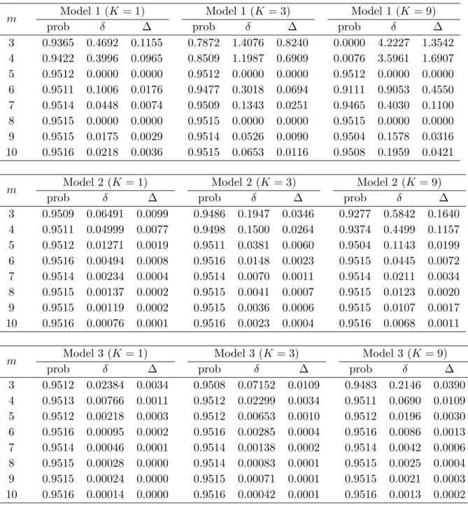
4.4.1 Coverage probability under model misspecification (1− α = 0.95) . . 26 4.4.2 Average band-width W (1− α = 0.95) . . . 27
vi
List of Figures
3.2.1 Tubes with a radius equal to the critical radius (Kuriki and Takemura,
2009). . . 12
4.3.1 Upper tail probability of the maximum of chi-square process Y (x). . . 22
4.3.2 Nominal confidence coefficient vs. Actual confidence coefficient. . . . 23
5.1.1 Average body weights of mice from four strains. . . 29
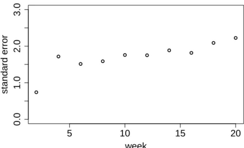
5.1.2 Estimated standard error bσ(xj). . . 30
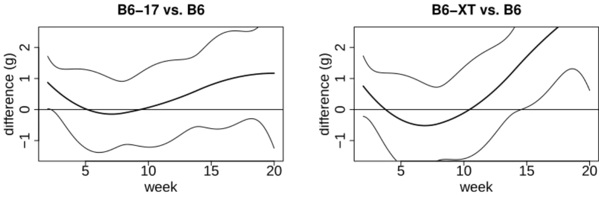
5.3.1 Differences of body weights and 95% confidence bands. . . 31
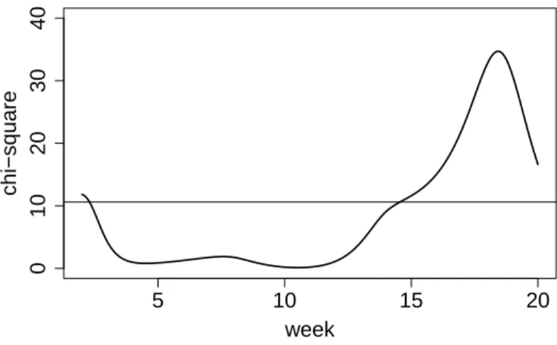
5.3.2 Chi-square process χ2(x) and its upper 5% critical value. . . 32
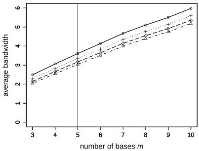
5.4.1 Confidence probability 1−α under basis vector f2,m. True model: m = 5. 33 5.4.2 Average bandwidth under basis vector f2,m. True model: m = 5. . . . 34
vii
Chapter 1
Introduction
Multiple regression analysis is a powerful technique used for predicting the relation- ship between a continuous random variable Y and several independent variables. Let Y1, Y2, . . . , Yp be a set of predictors believed to be related to a response variable Y . Let Y = (Y1, . . . , Yn)⊤ and xi = (x1i, . . . , xni)⊤ be the sequences of observations that follow the regression model.
Yj = β0+ β1xj1+ . . . + βpxjp+ εj, j = 1, . . . , n,
where βi, i = 0, 1, . . . , p are unknown regression coefficients and εj represents mutually independent N (0, σ2) random variables. We rewrite the regression model in matrix form as
Y = Xβ + ε,
where X = (1, x1, . . . , xp), β = (β0, β1, . . . , βp)⊤, ε = (ε1, . . . , εn)⊤, and 1 is a column vector of size n with all elements equal to one. The matrix X is defined as a design matrix. Without loss of generality, we assume that X is of full column rank.
For more details, see Anderson (2009).
1.1 Parameter estimation
The method of least squares estimation is a standard approach to estimating β in regression analysis. We can obtain the least squares estimator bβ of β by minimizing the least squares criterion, as in Liu (2010), given by
L(β) =||Y − Xβ||2 = (Y − Xβ)⊤(Y − Xβ).
1
1.2. Confidence intervals 2
Thus, the least squares estimator must satisfy
∂L(β)
∂β |β= bβ =−2X
⊤Y + 2X⊤X bβ = 0.
Because X is of full column rank, X⊤X is non-singular, and the normal equation leads to the least squares estimator
β = (Xb ⊤X)−1X⊤Y. Fitting the model, we can obtain
Y = X bb β = X(X⊤X)−1X⊤Y = HY,
where H = X(X⊤X)−1X⊤ is called the hat matrix such that H(I − H) = 0 since H2 = H.
The vector of residuals is defined as b
ε = Y − bY = (I− H)Y. The estimator bσ2 of σ2 is defined as
bσ2 =||bε||2/(n− p − 1).
Because y is a realization of a random vector Y with E(Y ) = Xβ, we obtain the following theorem.
Theorem 1.1.1. Under the standard normality assumptions, we have the following properties.
(i) bβ ∼ Np+1(β, σ2(X⊤X)−1). (ii) bε∼ Nn(0, σ2(I− H)). (iii) bσ2 ∼ n−p−1σ2 χ2n−p−1.
(iv) bβ and ε are independent.b (v) bβ and bσ2 are independent.
1.2 Confidence intervals
It is clear that x⊤β can be estimated by x⊤β, sinceb
x⊤( bβ− β) ∼ N (0, σ2x⊤(X⊤X)−1x).
1.3. The layout of this thesis 3
When σ is known,
x⊤( bβ− β) σ√x⊤(X⊤X)−1x
follows a normal distribution. Hence, a 1− α confidence interval for x⊤β is given by Pr{x⊤β ∈ x⊤βb± Zα/2σ√x⊤(X⊤X)−1x}= 1− α,
where Zα/2 is the upper α/2 point of the normal distribution.
When σ is unknown, it follows from Theorem 1.1.1 that β is independent of bσ. x⊤( bβ− β)
bσ√x⊤(X⊤X)−1x
follows a t distribution with n− p − 1 degrees of freedom. Hence, a 1 − α confidence interval for x⊤β is given by
Pr{x⊤β ∈ x⊤βb± tα/2bσ√x⊤(X⊤X)−1x}= 1− α,
where tα/2 is the upper α/2 point of the t distribution with n − p − 1 degrees of freedom, as in Liu (2010).
1.3 The layout of this thesis
The following is a brief outline of this thesis. Chapter 1 provides a brief review of mul- tiple regression models. In Chapter 2, we review simultaneous confidence bands for simple and multiple regression models, and we then address the problem of the con- struction of simultaneous confidence bands for nonlinear regression models. Chapter 3 looks at the volume-of-tube method, and we summarize the volume-of-tube method for evaluating the upper tail probability of the maximum of a Gaussian random field. The volume-of-tube method and its related method, referred to as the expected Euler- characteristic heuristic, are briefly summarized in Chapter 3. In Chapter 4, we define a Gaussian random field and a chi-square random process as pivotal quantities. We show that the critical value is determined from the upper tail probability of the max- imum of a Gaussian random field or a chi-square random process. The main results are provided in Chapter 4. Then, we discuss a simulation study under model mis- specification. Chapter 5 is devoted to the analysis of growth curve data. Chapter 6 considers the statistical parametric mapping approach as future work. Details of the proofs are in the Appendix.
Chapter 2
Simultaneous Confidence Bands
Simultaneous confidence bands are useful statistical inferential tools that can be used in many statistical branches. In this chapter, we summarize simultaneous confidence bands for simple and multiple regression models.
2.1 Confidence bands for one simple regression model
It is an important task to assess where the true model x⊤β lies in regression analysis from which the observed data have been generated.
When σ is known, a 1− α confidence region β is given by {
β : (β− bβ)
⊤(X⊤X)(β− bβ)
(p + 1)σ2 ≤ χ
2α(p + 1)
} ,
where χ2α(p + 1) is the upper α point of the χ2 distribution with p + 1 degrees of freedom.
When σ is unknown, a 1− α confidence region β is given by {β : (β− bβ)⊤(X⊤X)(β− bβ)
(p + 1)||Y − X bβ||2/(n− p − 1) ≤ f
α
p+1,n−p−1
},
where fp+1,n−p−1α is the upper α point of the F distribution with degrees of freedom of p + 1 and n− p − 1.
4
2.2. Confidence bands for one multiple regression model 5
2.2 Confidence bands for one multiple regression
model
The most well-known simultaneous confidence band of level 1− α for the regression model x⊤β for all x ∈ Rp is given by Hotelling (1951) and Scheff´e (1953, 1959). Working and Hotelling (1929) generalizes the band for a simple linear regression model. When σ is known,
x⊤β ∈ x⊤βb±√χ2α(p + 1)σ√x⊤(X⊤X)−1x. When σ is unknown,
x⊤β ∈ x⊤βb±√(p + 1)fp+1,n−p−1α bσ√x⊤(X⊤X)−1x.
The lower parts and the upper parts of the band are symmetric about the fitted model x⊤β.b
2.3 Confidence bands for more than two multiple
regression models
Suppose k linear regression models are defined as follows Yi = Xiβi+ εi, i = 1, . . . , k,
where Yi = (yi,1, . . . , yi,ni)⊤is a vector of random observations, Xi is a ni× (p + 1) full column-rank design matrix with the lth (1 ≤ l ≤ n) row given by (1, xl,1, . . . , xl,p), βi = (βi,0, . . . , βi,p)⊤, and εi = (εi,1, . . . , εi,n) with all the εi,j, j = 1, . . . , ni, i = 1, . . . , k being independent and identically distributed (i.i.d.) N (0, σ2) random variables. Si- multaneous confidence bands for all of the contrasts between the k regression models are given as
∑k i=1
cix⊤βi, for all c = (c1, . . . , ck)⊤∈ C,
where C is the set of all contrasts
C ={c = (c1, . . . , ck)⊤∈ Rk :
∑k i=1
ci = 0}.
2.4. Comparisons of nonlinear regression curves 6
When σ is known,
∑k i=1
cix⊤βi ∈
∑k i=1
cix⊤βbi± cασ vu ut∑k
i=1
c2ix⊤(Xi⊤Xi)−1x, ∀x ∈ Rp+1, ∀c ∈ C.
When σ is unknown,
∑k i=1
cix⊤βi ∈
∑k i=1
cix⊤βbi± dαbσ
vu ut∑k
i=1
c2ix⊤(Xi⊤Xi)−1x, ∀x ∈ Rp+1, ∀c ∈ C,
where cα and dα are determined by simulations. This provides a set of simultaneous confidence bands for all of the contrasts between the k regression models.
2.4 Comparisons of nonlinear regression curves
Considering multiple comparisons of k (≥ 3) nonlinear (curvilinear) regression curves estimated from independent k groups. Suppose that for each group i = 1, . . . , k, and for each explanatory variable xj ∈ X , j = 1, . . . , n, we have observations yij1, . . . , yijri
as objective variables with ri replications, which are assumed to follow the model yijh = gi(xj) + εijh, i = 1, . . . , k, j = 1, . . . , n, h = 1, . . . , ri. (2.4.1) Here, X ⊆ R is the domain of explanatory variables, and random errors εijh are assumed to be independently distributed as the normal distribution N (0, σ(xj)2). The variance function σ(x)2 is supposed to be known, or at least known up to a constant σ(x)2 = σ2σ0(x)2. In the case of the latter, we suppose that an independent estimator bσ2 of σ2 is available. In addition, we assume that the true regression curve has the form
gi(x) = βi⊤f (x), x∈ X , (2.4.2) where f (x) = (f1(x), . . . , fp(x))⊤is a known regression basis vector function, and βi = (βi1, . . . , βip)⊤ is an unknown parameter vector. Then, the least squares estimator bβi
of βi has the multivariate normal distribution Np(βi, r−1i Σ), where
Σ = ( n
∑
j=1
1
σ(xj)2f (xj)f (xj)
⊤
)−1
is the inverse of the p× p information matrix. When σ(x)2 = σ2σ0(x)2, we have Σ = σ2Σ0, where Σ0 is Σ with σ(xj) replaced by σ0(xj).
2.5. The problem we considered 7
LetC denote the set of vectors c = (c1, . . . , ck)⊤ such that ∑ki=1ci = 0. The focus of this thesis is the construction of 1− α simultaneous confidence bands for all the contrasts∑ki=1cigi(x) = ∑ki=1ciβi⊤f (x) between the k regression curves for all x∈ X and c∈ C, where X is a given finite interval [a, b], a finite union of intervals ⊔i[ai, bi],
or an infinite interval (−∞, ∞), with the symbol ‘⊔’ denoting a disjoint union. Specifically, according to the traditional form of the point estimate plus or mi- nus a probability point times the estimated standard error, we construct a 1− α simultaneous confidence band of the form
∑k i=1
ciβi⊤f (x)∈
∑k i=1
ciβbi⊤f (x)± b1−α vu ut
( k
∑
i=1
c2i ri
)
f (x)⊤Σf (x), (2.4.3)
where bβi⊤f (x) is the estimator of βi⊤f (x) in (2.4.2). This form is referred to as a hyperbolic-type (Liu, 2010). The critical value b1−α is determined such that the event in (2.4.3) for all x∈ X and c ∈ C holds with a probability of at least 1 − α. Our problem typically arises from growth curve analysis and longitudinal data analysis.
Throughout this paper, we assume that the regression curve gi(x) is a linear combination of a finite number of known basis functions in (2.4.2). Although it is a conventional regression model, we must always be careful regarding the approximation bias caused by model misspecification. This issue is examined in Section 4.4.
2.5 The problem we considered
The problem concerning the construction of simultaneous confidence bands in a re- gression model originates with Working and Hotelling (1929). They formalized this problem as the construction of confidence intervals for an estimated regression line, and provided a critical value by making use of the Cauchy-Schwarz inequality. Specif- ically, Working and Hotelling (1929) treated the case of
(i) one regression model (equivalent to case k = 2 in our problem), (ii) the simple regression f (x) = (1, x)⊤, and
(iii) the unrestricted domain of the explanatory variables X = (−∞, ∞).
Subsequently, many reports concerning the relaxation of these conditions have ap- peared in literature.
In the case of one regression model, Wynn and Bloomfield (1971) pointed out that the use of the Cauchy-Schwarz inequality leads to conservative bands unless both (ii) and (iii) hold. They illustrated improved confidence bands for the quadratic regression f (x) = (1, x, x2)⊤. Uusipaikka (1983) constructed exact confidence bands for linear regression when X is a finite interval. See Liu, Lin, and Piegorsch (2008) and Liu
2.5. The problem we considered 8
(2010) for historical reviews. The problem of k ≥ 3 regression curve comparisons was considered by Spurrier (1999, 2002) and Lu and Chen (2009), who proposed procedures based on simple linear regression. However, it is difficult to extend these methods to nonlinear regression.
One exception is Naiman (1986)’s integral-geometric approach. In the unit sphere Sp−1 of the p-dimensional Euclidean space, he defined a trajectory
Γ ={ψ(x) | x ∈ X } ⊂ Sp−1 (2.5.1) of a normalized basis vector function
ψ(x) = Σ
1/2f (x)
∥Σ1/2f (x)∥, (2.5.2)
and evaluated the volume of the Γ tubular neighborhood. In the case of one regression model, he constructed a simultaneous confidence band with the critical value obtained from this volume. The volume formula for such tubes originated from Hotelling (1939) and Weyl (1939). Currently, this idea is understood in the volume-of-tube method framework (Adler and Taylor (2007), Kuriki and Takemura (2001), Kuriki and Takemura (2009), Sun (1993), Takemura and Kuriki (2002)). As shown in Section 4.1, we require the tail probability of the maximum of a Gaussian random field or chi-square random process as a pivotal quantity. Volume-of-tube is a methodology to evaluate such tail probabilities.
In this paper, we adopt this integral-geometric approach. In the case of k ≥ 3, we define a subset M in (4.2.1) of a unit sphere, and by evaluating the volume of its tubular neighborhood, we obtain the critical value b1−α in (2.4.3) by means of the volume-of-tube method. Moreover, we prove that the proposed confidence band is conservative. It is known that Naiman (1986)’s confidence band is conservative (Naiman’s inequality, see also Johnstone and Siegmund (1989)), and our result is regarded as its generalization.
Note that, in the setting of this paper, the covariance matrices of the estimators bβi
are identical up to a multiplicative constant. This property arises from the condition that the explanatory variables xj are common between k groups in the model (2.4.1). This represents the purported balanced case. For the unbalanced case, the problem of constructing simultaneous confidence bands is quite tedious and only simulation- based approaches are available (Jamshidian, Liu, and Bretz (2010), Liu (2010), Liu, Jamshidian, and Zhang (2004), Liu, Wynn, and Hayter (2008)). In this paper, we address only the balanced case.
Moreover, note that in the one-group case (k = 1), various simultaneous confi- dence bands by means of the volume-of-tube method have been proposed. Johansen and Johnstone (1990) demonstrated the usefulness of Hotelling’s volume formula for
2.5. The problem we considered 9
the construction of simultaneous bands. The application to the B-spline regression is found in Shen, Wolfe, and Zhou (1998). Sun and Loader (1994) proposed a modifica- tion to the volume-of-tube formula when a small approximation bias caused by model misspecification exists. In succeeding papers, Sun and her coauthors developed this idea further in various model settings (Faraway and Sun (1995), Sun, Loader, and McCormick (2000), Sun, Raz, and Faraway (1999)). See also Krivobokova, Kneib, and Claeskenset (2010). The crucial difference between this paper and existing work is that in this paper, we need to treat a Gaussian random field with a general dimen- sional (k− 1 dimensional) index set, and need the volume formula up to an arbitrary order.
Chapter 3
The Volume-of-Tube Method
3.1 Definition of the tube
Considering general case, let Sn−1= S(Rn) be the unit sphere in Rnand let M ⊂ Sn−1 be a closed subset of Sn−1. Let the elements of ξ = (ξ1, . . . , ξn) be independent and standard normal random variables. (We write this as ξ ∼ Nn(0, In).) ⟨·, ·⟩ denotes the standard inner product of Rn. Our problem is to find the distribution of the maximum of the Gaussian random field X(p) =⟨ξ, p⟩, p ∈ M :
Pr(max
p∈M⟨ξ, p⟩ ≥ c
)
. (3.1.1)
Definition 3.1.1 (Tube). The tube (spherical tube) of radius θ about M is defined to be the set of points on Sn−1 whose great-circle distance to M is less than or equal to θ :
Mθ ={q∈ Sn−1 | dist(q, M) ≤ θ}={v ∈ Sn−1 min
u∈Mcos
−1(u⊤v)≤ θ}.
For an n-dimensional standard normal random vector ξ ∼ Nn(0, In), its “length”
∥ξ∥ and its “direction” ζ = ξ/∥ξ∥ are independently distributed and the distribution of ζ is the uniform distribution over the unit sphere Unif(Sn−1). Hence,
Pr(max
p∈M⟨ξ, p⟩ ≥ c
)
=E [
Pr(max
p∈M⟨ζ, p⟩ ≥
c
∥ξ∥ | ∥ξ∥ )]
=E [
Pr(dist(ζ, M )≤ cos−1( c
∥ξ∥
)| ∥ξ∥)]
= 1
Vol(Sn−1)E
[Vol(Mcos−1(c/∥ξ∥)
)],
10
3.2. Definition of the critical radius 11
where Vol(·) is the (n − 1)-dimensional volume. If the volume of the tube Vol(Mθ) can be evaluated for every θ, then we can integrate it once (that is, we can take the expected value with respect to ∥ξ∥) to obtain the tail probability of the maximum (3.1.1).
3.2 Definition of the critical radius
The support cone (or tangent cone) of M at u∈ M is denoted by SuM . (See Section 1.2 of Takemura and Kuriki (2002) for the definition.) The cone with base set M is denoted by
co(M ) = ⊔
λ≥0
λM.
Then, the support cone of co(M ) at u ∈ M is decomposed as Su(co(M )) = SuM ⊕ span{u}, where span{u} is the linear space spanned by u. The normal cone of co(M) at u∈ M is defined by the dual of the support cone: Nu(co(M )) = Su(co(M ))∗. Definition 3.2.1 (Critical radius). We say that the tube Mθ does not have a self- intersection if every point q∈ Mθ\ M is uniquely written as
q = p cos ψ + v sin ψ, p∈ M, v ∈ Nu(co(M ))∩ Sn−1, ψ∈ (0, θ]. The supremum of the radius θ such that Mθ does not have a self-intersection
θc = sup{θ ≥ 0 | Mθ does not have a self-intersection}
is the critical radius (reach) of M (Figure 3.2.1). Let θc = π/2 when θc is more than π/2.
3.3. Volume-of-tube method and upper tail probability 12
M M
Figure 3.2.1: Tubes with a radius equal to the critical radius (Kuriki and Takemura, 2009).
3.3 Volume-of-tube method and upper tail proba-
bility
In this section, we summarize the volume-of-tube method for evaluating the upper tail probability of the maximum of a Gaussian random field.
Let ξ be a Gaussian random vector distributed as Nn(0, I). Let M be a closed subset of Sn−1, the unit sphere (the set of unit column vectors) of Rn. Then, the random map u 7→ ξ⊤u, u ∈ M, is a Gaussian random field with mean 0, variance 1, and a covariance function Cov(ξ⊤u, ξ⊤v) = u⊤v. The volume-of-tube method approximates the distribution of the maximum maxu∈Mξ⊤u. To apply the volume- of-tube method, we require the following assumption on M .
Assumption 3.3.1. M is a d-dimensional closed piecewise C2-manifold, or M is a d-dimensional C2-manifold with piecewise C2-boundary. We write M = IntM⊔ ∂M, where IntM and ∂M denote the interior and the boundary of M , respectively. In the former case, ∂M =∅.
Under Assumption 3.3.1, we can prove that θc > 0.
Note that the (m− 1)-dimensional volume of Sm−1 is Ωm = 2πm/2/Γ(m/2). For m× m matrix A = (aij), let tr0A = 1 and
treA = ∑
1≤k1<...<ke≤m
det(akikj)1≤i,j≤e, 1≤ e ≤ m
(Muirhead (2005), Appendix A.7). Note that tr1A = trA, trmA = det A. The upper probability of the chi-square distribution with m degrees of freedom is denoted by Gm(·). Now we can provide the upper tail probability formula for the Gaussian field ξ⊤u, u∈ M. The theorem below is a special case of Proposition 2.2 of Takemura and Kuriki (2002).
3.3. Volume-of-tube method and upper tail probability 13
Proposition 3.3.1. As b→ ∞, Pr
( maxu∈M ξ
⊤u≥ b
)
= Ptube(b) + O(Gn(b2(1 + tan2θc))), (3.3.1) where
Ptube(b) = ∑
0≤e≤d, e:even
wd+1−eGd+1−e(b2) + ∑
0≤e≤d−1
w′d−eGd−e(b2), (3.3.2)
with
wd+1−e= 1
Ωd+1−eΩn−d−1+e
∫
IntM
{∫
Nu(co(M ))∩Sn−1
treH(u, v) dv }
du, (3.3.3) wd−e′ = 1
Ωd−eΩn−d+e
∫
∂M
{∫
Nu(co(M ))∩Sn−1
treH′(u, v) dv }
du. (3.3.4)
Here, H(u, v) is the second fundamental form of IntM at u in the direction of v, and H′(u, v) is the second fundamental form of ∂M at u in the direction of v. du is the volume element of IntM or ∂M , and dv is the volume element of Nu(co(M ))∩ Sn−1.
In (3.3.1), because θc > 0, the error term O(Gn(b2(1+tan2θc))) = O(bn−2e−b2(1+tan2θc)/2) is exponentially smaller than each term Gj(b2) = O(bj−2e−b2/2). Hence, (3.3.2) can be used as an approximation formula when b is large. The method in which Ptube(b) is used as an approximate value is referred to as the volume-of-tube method, or simply, the tube method. This name comes from the volume formula for Mθ below.
Remark 3.3.1. For the radius θ∈ [0, θc], the (n− 1)-dimensional spherical volume of the tube Mθ is given by
Voln−1(Mθ) = Ωn
{ ∑
0≤e≤d, e:even
wd+1−eB1
2(d+1−e),12(n−d−1+e)(cos
2θ)
+ ∑
0≤e≤d−1
w′d−eB1
2(d−e), 1
2(n−d+e)(cos
2θ)
} ,
where wd+1−eand wd−e′ are given in (3.3.3) and (3.3.4), Ba,b(·) is the upper probability of the beta distribution with parameter (a, b).
The critical radius θccan be evaluated using the following characterization (Theo- rem 4.18 of Federer (1959), Proposition 4.3 of Johansen and Johnstone (1990), Lemma 2.2 of Takemura and Kuriki (2002)). For a proof, see Theorem 2.9 of Kuriki and Take- mura (2009).
3.4. Expected Euler-characteristic heuristic 14
Proposition 3.3.2. The critical radius θc of M is given by tan2θc = inf
u̸=v∈M
(1− u⊤v)2
∥Pv⊥(u− v)∥2, (3.3.5) where Pv⊥ is the orthogonal projection onto the normal cone Nv(co(M )) of co(M ) at v.
The local critical radius θc,loc is defined as tan2θc,loc = lim inf
u̸=v∈M, ∥u−v∥→0
(1− u⊤v)2
∥Pv⊥(u− v)∥2. (3.3.6) From the definition, it holds that θc ≤ θc,loc. In general, θc,loc is easier to evaluate than θc.
3.4 Expected Euler-characteristic heuristic
We have summarized the volume-of-tube method to evaluate the upper tail probabil- ities of the maximum of random fields thus far. There is another method utilized for the same purpose, known as the expected Euler-characteristic heuristic (Adler and Taylor (2007), Worsley (1995)). When applied to the Gaussian random field ξ⊤u, u∈ M, this method is stated as follows: For each b, define the excursion set by
Ab ={u ∈ M | ξ⊤u≥ b}.
Let χ(·) be the Euler-Poincar´e characteristic of a set, and 1(·) be the indicator function for an event. The expected Euler-characteristic heuristic assumes that 1(Ab ̸= ∅) ≈ χ(Ab) for large b, and
Pr (
maxu∈M ξ
⊤u≥ b
)
= E{1(Ab ̸= ∅)} ≈ E{χ(Ab)}.
Note that χ(Ab) can be evaluated by Morse’s theorem, and is more tractable than 1(Ab ̸= ∅). Takemura and Kuriki (2002) proved the equivalence of the volume-of-tube method and expected Euler-characteristic heuristic as follows.
Proposition 3.4.1 (Proposition 3.3 of Takemura and Kuriki (2002)). E{χ(Ab)} = Ptube(b), for all b≥ 0.
Using this, Takemura and Kuriki (2002) provided an alternative proof that the confidence band of Naiman (1986) is conservative.
Chapter 4
Construction of Simultaneous
Confidence Bands
4.1 Random fields as pivotal quantities
Our problem is to determine the critical value b1−α in (2.4.3). First, assume that Σ is fully known. Define a pivotal quantity:
T (x, c) =
∑k
i=1ci( bβi− βi)⊤f (x)
√(∑k i=1
c2i ri
)f (x)⊤Σf (x)
. (4.1.1)
Then, the critical value b1−α is solution b of the equation: Pr{T (x, c)≤ b, ∀x ∈ X , ∀c ∈ C}= Pr
{
x∈X ,c∈Cmax T (x, c)≤ b }
= 1− α.
In this expression, we use T (x, c) instead of |T (x, c)|, because c ∈ C implies −c ∈ C and|T (x, c)| is equal to T (x, c) or T (x, −c). Inverting |T (c, x)| ≤ b1−α yields the 1−α simultaneous confidence band in (2.4.3).
In the following, we show that b21−α is the upper α point of the maximum of a chi-square random process. We can assume that ∑ki=1c2i/ri = 1 without the loss of generality, because T (x, c) is a homogeneous function in c. Let ρ = (√r1, . . . , √rk)⊤, and define a k× (k − 1) matrix H such that ρ⊤H = 0, H⊤H = Ik−1, and HH⊤ =
Ik − ρρ⊤/(ρ⊤ρ). (An example of H is given in Remark 4.2.1 below.) Then, the c = (c1, . . . , ck)⊤ such that∑ki=1c2i/ri = 1 and∑ki=1ci = 0 are represented as
c = diag(√r1, . . . ,√rk)Hh, h∈ Sk−2,
15
4.1. Random fields as pivotal quantities 16
where Sk−2 is the set of (k− 1)-dimensional unit column vectors.
Let Σ1/2 be a matrix such that (Σ1/2)⊤Σ1/2 = Σ, and let Σ−1/2 be its inverse. Then, ηi = √ri(Σ−1/2)⊤( bβi− βi) is distributed normally as Np(0, I), independently for i = 1, . . . , k. Let ψ :X → Sp−1 as defined in (2.5.2). Then, T (x, c) is rewritten as
T (x, c) =
∑k i=1
ci
√r
i
√ri{(Σ−1/2)⊤( bβi− βi)}⊤ Σ
1/2f (x)
∥Σ1/2f (x)∥
=c⊤diag(√r1, . . . ,√rk)−1
η⊤1
... η⊤k
k×p
ψ(x)
=h⊤
ξ1⊤
... ξk−1⊤
(k−1)×p
ψ(x)
=ξ⊤{h ⊗ ψ(x)}, (4.1.2)
where ξi are p× 1 vectors defined by (ξ1, . . . , ξk−1)p×(k−1) = (η1, . . . , ηk)p×kH, ξ = (ξ1⊤, . . . , ξk−1⊤ )⊤ is a p(k− 1) × 1 vector, and ‘⊗’ is the Kronecker product. Vectors ηi consist of independent standard Gaussian random variables N (0, 1), therefore, so does vector ξ. When x and h are fixed, because ∥ψ(x)∥ = ∥h ⊗ ψ(x)∥ = 1, ξi⊤ψ(x) is
distributed asN (0, 1) independently for i = 1, . . . , k, and ξ⊤{h ⊗ ψ(x)} is distributed as N (0, 1).
From (4.1.2), we can see that
maxc∈C T (x, c) =
vu ut∑k−1
i=1
{ξi⊤ψ(x)}2. (4.1.3)
For each fixed x, this is distributed as the square root of the chi-square distribution χ2k−1 with k− 1 degrees of freedom.
When Σ = σ2Σ0 with Σ0 known, and an independent estimator bσ2 ∼ σ2χ2ν/ν of unknown σ2 is available, we redefine T (x, c) in (4.1.1) by replacing Σ in the denomi- nator with bσ2Σ0. Thus, instead of (4.1.2) and (4.1.3) we have
T (x, c) = 1 τξ
⊤{h ⊗ ψ(x)}, max
c∈C T (x, c) =
vu ut 1
τ2
∑k−1 i=1
{ξi⊤ψ(x)}2, τ2 = bσ
2
σ2.
4.2. Tube formula 17
4.2 Tube formula
In the particular case of the problem we consider, the maximum of Z(x, h) in (4.2.2) can be treated in this framework by setting
M = {h ⊗ ψ(x) | (x, h) ∈ X × Sk−2} and n = p(k − 1). (4.2.1) The dimension of M is d = dim M = k− 1.
When M is defined by (4.2.1), we can provide a sufficient condition for Assumption 3.3.1.
Assumption 4.2.1. ψ :X → Sp−1 is a one-to-one map of class piecewise C2. There does not exist x, ˜x∈ X such that ψ(x) = −ψ(˜x).
Under Assumption 4.2.1, the map (x, h)7→ h ⊗ ψ(x) is a piecewise C2 one-to-one map.
Example 4.2.1. Consider the polynomial regression with a basis function vector f (x) = (1, x, . . . , xp−1)⊤. When the domain of x is a finite interval X = [a, b], we have
IntM ={h ⊗ ψ(x) | x ∈ (a, b), h ∈ Sk−2},
∂M ={h ⊗ ψ(a) | h ∈ Sk−2} ⊔ {h ⊗ ψ(b) | h ∈ Sk−2}. When X = (−∞, ∞), ψ(±∞) = (±1)p−1Σ1/2ep/
√e⊤pΣep with ep = (0, . . . , 0, 1)⊤, and hence h⊗ ψ(∞) = (−1)p−1h⊗ ψ(−∞). This denotes that M is a closed manifold without boundary.
Example 4.2.2. Consider the trigonometric regression with a basis function vector f (x) =(1,√2 cos x,√2 sin x, . . . ,√2 cos mx,√2 sin mx)⊤.
When X = [0, 2π), M is a closed manifold without boundary.
Now, we consider the object in (4.1.2) as a random function of (x, h):
Z(x, h) = ξ⊤{h ⊗ ψ(x)}, (x, h) ∈ X × Sk−2, (4.2.2) where ξ ∼ Np(k−1)(0, I). Then, Z(x, h) is the Gaussian random field with mean 0, variance 1, and covariance function
Cov[Z(x, h), Z(˜x, ˜h)]= ψ(x)⊤ψ(˜x)· h⊤˜h.
4.2. Tube formula 18
Similarly, we define the chi-square random process with k− 1 degrees of freedom:
Y (x) =
∑k−1 i=1
{ξi⊤ψ(x)}2, x∈ X . (4.2.3)
We summarize the results of this section below.
Theorem 4.2.1. When Σ is known, the critical value b1−α is determined as the solution b = b1−α of
Pr {
x∈X ,h∈Smaxk−2Z(x, h)≥ b }
= Pr {
maxx∈X Y (x)≥ b 2
}
= α,
where Z(x, h) is the Gaussian random field defined in (4.2.2), and Y (x) is the chi- square random process defined in (4.2.3).
When Σ = σ2Σ0 with Σ0 known, the critical value b1−α is determined as the solution b = b1−α of
E [
Pr {
x∈X ,h∈Smaxk−2Z(x, h)≥ bτ
τ2}]= E [
Pr {
maxx∈X Y (x)≥ b
2τ2 τ2
}]
= α, where the expectation is taken over τ2 ∼ χ2ν/ν, with ν being the degrees of freedom of the estimator of σ2.
Remark 4.2.1. An example of k×(k−1) matrix H such that ρ⊤H = 0, H⊤H = Ik−1,
HH⊤= Ik− ρρ⊤/(ρ⊤ρ) with ρ = (√r1, . . . , √rk)⊤ is given as
H =
√r
1r2
√R1R2
√r
1r3
√R2R3 . . .
√r
1rk
√Rk−1Rk
−√RR11R2 √√Rr22rR33 . . . √√Rr2rk
k−1Rk
−√RR22R3 . . . √√Rr3rk
k−1Rk
. .. ...
0 −√Rk−1
Rk−1Rk
k×(k−1)
,
where Ri =∑ij=1rj.
Theorem 4.2.2. Let ξ ∼ Nn(0, I), n = p(k − 1). Let Γ ⊂ Sp−1 and M ⊂ Sn−1 be defined by (2.5.1) and (4.2.1), and let|Γ| denote the length of Γ. Assume Assumption
4.2. Tube formula 19
4.2.1 on ψ. Then, as b→ ∞, Pr
{
(x,h)∈X ×Smaxk−2Z(x, h)≥ b }
= Pr {
maxx∈X Y (x)≥ b 2
}
= Pr (
maxu∈M ξ
⊤u≥ b
)
=Ptube(b) + O(bn−2e−(1+tan2θc)b2/2), where
Ptube(b) = Γ(
k 2)
√π Γ(k−12 )|Γ|
{Gk(b2)− Gk−2(b2)}+ χ(Γ)Gk−1(b2). (4.2.4)
Note that if Γ (and hence M ) has no boundary, then Γ is homeomorphic to S1, and therefore χ(Γ) = 0. Otherwise, χ(Γ) is the number of connected components of Γ. Theorem 4.2.3. Assume Assumption 4.2.1. Suppose that Γ has boundaries. The approximation formula given in Theorem 4.2.2 is a conservative bound, specifically,
Pr (
maxu∈M ξ
⊤u≥ b
)
≤ Ptube(b) for all b≥ 0.
Proof. Arrange the p(k− 1) × 1 vector ξ = (ξ⊤1, . . . , ξk−1⊤ )⊤, and define a (k− 1) × p matrix Ξ = (ξ1, . . . , ξk−1)⊤. Let
Ab ={u ∈ M | ξ⊤u≥ b} = {h ⊗ q | (q, h) ∈ Γ × Sk−2, h⊤Ξq ≥ b} ⊂ Sp(k−1)−1, Aeb ={(q, h) ∈ Γ × Sk−2 | h⊤Ξq ≥ b} ⊂ Sp−1× Sk−2,
Bb ={q ∈ Γ | q⊤Ξ⊤Ξq ≥ b2} ⊂ Sp−1.
Note that Ab is the excursion set of the Gaussian random field ξ⊤u, u ∈ M, eAb is the excursion set of the Gaussian random field ∑k−1i=1 hi(ξi⊤q) = h⊤Ξq, (q, h) ∈ Γ × Sk−2, and Bb is the excursion set of the chi-square random process∑k−1i=1(ξi⊤q)2 = q⊤Ξ⊤Ξq, q ∈ Γ. We will prove that for each fixed ξ, 1(Ab ̸= ∅) = 1( eAb ̸= ∅) = 1(Bb ̸= ∅) and χ(Ab) = χ( eAb) = χ(Bb).
First, note that owing to Assumption 4.2.1, the map (q, h)7→ h ⊗ q is one-to-one. Hence, Ab and eAb are homeomorphic and therefore 1(Ab ̸= ∅) = 1( eAb ̸= ∅) and χ(Ab) = χ( eAb).
Moreover, noting that eAb ̸= ∅ ⇔ maxhh⊤Ξq ≥ b for some q ⇔ q⊤ΞΞ⊤q ≥ b2 for
4.2. Tube formula 20
some q ⇔ Bb ̸= ∅, that is, 1( eAb ̸= ∅) = 1(Bb ̸= ∅), we can write Aeb = ⊔
q∈Bb
{(q, h) | h ∈ Sk−2, h⊤Ξq ≥ b}.
Given b≥ 0, the set {h ∈ Sk−2 | h⊤Ξq ≥ b} is contractible and star-shaped about the point h∗(q) = Ξq/∥Ξq∥. That is, the map
ϕ : eAb× [0, 1] → eAb, (q, h, t)7→ (
q, (1− t)h + th∗(q)
∥(1 − t)h + th∗(q)∥ )
is continuous, and ϕ( eAb × {0}
) = eAb is homotopy equivalent to the set ϕ( eAb ×
{1}) = ⊔q∈Bb{(q, h∗(q))}. This is homotopy equivalent to ⊔q∈Bb{q} = Bb. Hence, χ( eAb) = χ(Bb).
Recall that Bb is the excursion set of the chi-square random process on the one- dimensional index set Γ. This means that Bb is also one-dimensional, and χ(Bb) is only the number of connected components of Bb. Therefore 1(Bb ̸= ∅) ≤ χ(Bb). By
taking expectations, Pr
( maxu∈M ξ
⊤u≥ b
)
= E{1(Ab ̸= ∅)} = E{1(Bb ̸= ∅)}
≤ E{χ(Bb)} = E{χ(Ab)} = Ptube(b). The last equality is owing to Proposition 3.4.1.
Remark 4.2.2. Naiman (1986) proved that application of the volume-of-tube method to a Gaussian random process with a one-dimensional index set always provides a conservative band. Theorem 4.2.3 is a generalization of Naiman (1986)’s inequality to a chi-square random process.
Theorem 4.2.4. The interior and boundary of Γ are denoted by IntΓ and ∂Γ, re- spectively. The critical radius θc of M is given by
tan2θc = min {
x̸=˜x, ψ(x)∈IntΓinf
(1− αs)2
1− s2− α2t2,x̸=˜x, ψ(x)∈∂Γinf
(1− αs)2
1− s2 − max{0, ε(x)αt}2 }
, where the infima are taken over x, ˜x ∈ X , and α ∈ [−1, 1] as well as additional conditions (arguments of inf), and
s = s(x, ˜x) = ψ(x)⊤ψ(˜x), t = t(x, ˜x) = ψx(x)⊤ψ(˜x)
∥ψx(x)∥ ,
4.3. A numerical example 21
ψx(x) = ∂ψ(x)/∂x,
ε(x) =
{1 (ψx(x) is inward to Γ),
−1 (ψx(x) is outward to Γ).
ψx(x) is said to be inward or outward to Γ if the support cone of Γ at ψ(x) is Sψ(x)Γ = {λψx(s)| λ ≥ 0} or {λψx(s)| λ ≤ 0}, respectively.
Theorem 4.2.5. Assume Assumption 4.2.1. Moreover, assume that ψ : X → Sp−1 is of C4-class. Then, the local critical radius θc,loc is given by
tan2θc,loc = min {
x∈X :κ(x)≤2inf {
1− κ(x) 4
}
, inf
x∈X :κ(x)≥2
1 κ(x)
}
with
κ(x) = ψxx(x)⊤ψxx(x) {ψx(x)⊤ψx(x)}2 −
{ψxx(x)⊤ψx(x)}2
{ψx(x)⊤ψx(x)}3 − 1, (4.2.5) where ψx(x) = ∂ψ(x)/∂x and ψxx(x) = ∂2ψ(x)/∂x2.
The proofs of Theorems 4.2.4 and 4.2.5 are included in the Appendix.
4.3 A numerical example
In this section, we provide a numerical example to determine the accuracy of the approximation formula given in Theorem 4.2.2, and degree of conservativeness proved by Theorem 4.2.3.
Suppose that f (x) = (1, x, x2)⊤, X = [−1, 1], and
Σ =
1 0
2
0 23 03 2
3 0 1
, Σ1/2 =
1 0 23 0 √23 0 0 0 √35
.
Then,
ψ(x) = 1 3(1 + x2)
(3 + 2x2,√6x,√5x2)⊤, |Γ| =
∫
X ∥ ˙ψ(x)∥ dx =
∫ 1
−1
√2 3
1
1 + x2 dx =
√π 6. κ(x) in (4.2.5) is always 5. Hence, the local critical radius is θc,loc = tan−1(1/√5) = 0.134π. Further, we can also confirm that the critical radius is the same as θc= θc,loc using Mathematica (Wolfram Research, Inc., 2016).