Competition in Treasury Auctions
∗
Helmut Elsinger
†Philipp Schmidt-Dengler
‡Christine Zulehner
§February 2017
Abstract
We investigate the role of competition on the outcome of Austrian Treasury auctions. Austria’s EU accession led to an increase in the number of banks partici-pating in treasury auctions. We use structural estimates of bidders’ private values to examine the effect of increased competition on auction performance. We find that bidders’ surplus dropped sharply after EU Accession, but less than reduced form estimates would suggest. A significant component of the surplus reduction is due to aggressive bidding and cannot only be explained by increased bidder num-bers resulting in more draws of bidder valuations. Counterfactuals establish that as competition increases, concerns regarding auction format play a smaller role. JEL Classifications: D44, G12, G21, L10, L13
Keywords: treasury auctions, multi-unit auctions, independent private values, com-petition, bidder surplus, auction format
∗We wish to thank the Austrian Treasury (Oesterreichische Bundesfinanzierungsagentur – OeBFA)
and the Oesterreichische Kontrollbank (OeKB) for data provision. Isis Durrmeyer, Paul Kocher, Maria Kucera, Oren Rigbi, Frank Rosar, Erich Weiss and seminar participants at Copenhagen Business School, Frankfurt, Northwestern, SciencePo, St. Gallen, Stockholm School of Economics, Toulouse, Vienna, Wuerzburg, Zurich, CEPR, EARIE, EEA, MaCCI and NOeG provided helpful comments and sugges-tions. The views expressed are entirely those of the authors and do not necessarily represent those of Oesterreichische Nationalbank. Schmidt-Dengler thanks DFG for financial support through SFB/TR 15. Christine Zulehner gratefully acknowledges support from the Research Center SAFE, funded by the State of Hessen initiative for research LOEWE.
†Oesterreichische Nationalbank, Address: Otto-Wagner-Platz 3, A-1090 Vienna, Austria, Email:
hel-mut.elsinger@oenb.at.
‡University of Vienna, also affiliated with CEPR, CES-Ifo, WIFO and ZEW, Address:
Oskar-Morgenstern-Platz 1, A-1090 Vienna, Austria, Email: philipp.schmidt-dengler@univie.ac.at.
§Goethe-University Frankfurt, also affiliated with CEPR, SAFE Research Center and WIFO,
zulehner@safe.uni-1
Introduction
To issue treasury securities by auctions is a common method to raise money for government
expenditures in many countries over the world. The auction mechanisms used vary across
countries. In this study, we analyze the bidding behavior in Austrian Treasury bond
auctions, using data containing all bids submitted by each bidder between February 1991
and May 2008.
The empirical literature on security auctions has focused on the question of the
appro-priate auction design (uniform versus discriminatory, see Fevrier et al. (2004), Horta¸csu
and McAdams (2010), Kastl (2011)) and the informational environment (independent
private versus affiliated/common values, see Horta¸csu and Kastl (2012)). While our
mod-eling and estimation approach closely follows the aforementioned papers, this paper asks
a different question. We examine to what extent the increased competition resulting from
EU accession affected auction performance.
Before Austria’s EU accession, only Austrian banks were allowed to participate in
Austrian Treasury Auctions. EU accession in 1995 led to an increase in the number of
banks participating in the bidding process. While on average 13 bidders participated in
Austrian treasury auctions before 1995, this number increased to almost 25 between 1997
and 2008. By employing the resampling techniques suggested in Horta¸csu and McAdams
(2010) and Kastl (2011), we obtain estimates of bidders’ valuations of the auctioned bonds
for the periods before and after EU Accession respectively. Based on these estimates, we
examine the surplus obtained by bidders in the two different time periods. We find that
the Austrian government benefited from increased competition in the bidding process for
its debt issues. The surplus left to bidding banks was reduced by about three basis points
or eighty percent (corresponding to 0.7 million euro per auction). We decompose the
change in surplus resulting from increased competition into a strategic effect, due to more
aggressive bidding, and a statistical effect, resulting from the larger number of draws of
bidder valuations. We find that the pure statistical effect can only account for half of the
We also compare the structural estimates with results from difference-in-difference
estimates that treat EU accession as a quasi-experiment using German bond yields as a
control group. The difference-in-difference estimates find a much larger effect suggesting
that EU accession lead to a 50 basis point reduction in yields. We provide an explanation
for the discrepancy of results, by comparing our structural estimates of bidders’ valuations
relative to German yields before and after EU accession. This comparison establishes
that a large fraction of the estimated reduced form effect is due to a change in valuations:
Valuations have increased relative to German yields by around 40 basis points after EU
accession.
Finally, we use our estimates to perform counterfactuals along the lines of Horta¸csu
and McAdams (2010) to illustrate the effect of changing the format to a hypothetical
uniform auction. We show that this alternative format would have increased government
revenue before EU accession. With increased competition, the choice of auction format
plays a much smaller role, both in terms of revenue as well as allocative efficiency, but
from a government’s perspective the discriminatory auction would be slightly better.
How the number of competitors affects the level of competition and market outcomes
more broadly is a long standing question. See for instance Weiss (1989)’s review of
the effect of the number of firms on market price. The question is reflected in Selten
(1973)’s finding that “four are few and six are many” referring to the number of firms
that separates a small group of firms from a large one. This has been followed by a series of
laboratory experiments (e.g. Huck et al. (2004)), but only little research was done on
non-experimental data where the number of potential competitors has changed exogenously.
Closely related to our work is the analysis of entry into local markets by Bresnahan
and Reiss (1991), who find that competitive conduct changes quickly as the number
of incumbents increases with increasing market size. We contribute to this literature by
comparing the outcome of treasury auctions in two different episodes with different bidder
numbers.
environment of Austrian treasury auctions. We describe the data, provide evidence of the
increased competition on the outcomes of Austrian treasury auctions and results from
difference-in-difference regressions. Section 3 presents the bidding model and estimation
technique as well as estimation results. Section 4 presents our analysis of the effect of
competition on bidder surplus, the auction format and efficiency. Section 5 concludes.
2
Austrian Treasury Auctions
Since 1991 Austrian Treasury bonds have been sold through sealed, multiple-bid,
discrim-inatory yield tenders or price auctions. Treasury auctions are organized by the
Oesterre-ichische Kontrollbank AG (OeKB). OeKB holds the auctions on behalf of the Austrian
Treasury (Oesterreichische Bundesfinanzierungsagentur – OeBFA), the debt management
office of the Republic of Austria. New bonds may be issued through yield tenders, price
auctions or through a syndicate of banks. Whereas new issues prevailed in the 1990s,
trea-sury policy now focuses on reopening existing instruments to enhance their liquidity. New
securities are issued only occasionally (one or two issues per year) to close gaps in traded
maturities. In the recent past these securities were issued through a syndicate of banks.
In 2001, the OeBFA switched from using yield tenders to price auctions when
reopen-ing an existreopen-ing instrument. Participation in these auctions is managed by the OeBFA.
Banks meeting certain requirements in terms of capital, number of employees, number
of branches, and trading volume in euro-denominated government bonds are eligible to
apply for participation. Upon approval by the OeBFA, bidders not only may, but must
submit competitive bids in every auction. The identity of currently approved banks is
public information through the OeKB.
Treasury auctions are held approximately every six weeks. At the end of the calendar
year, a preliminary schedule for the coming year is published. One week before each
auc-tion, the OeBFA announces the characteristics of the bond to be auctioned, i.e. maturity,
(usually a Tuesday). The issuer has the right to recall the auction until noon.
The bids must be submitted in denominations of euro 1 million or a multiple thereof
containing the yield or the price at which the bidder is prepared to accept the nominal
amount. Multiple bids are allowed. Bids may be modified and submitted up to the
deadline as often as desired. The minimum total volume an approved bank is obliged
to bid corresponds to the issue size announced by the issuer divided by the number of
auction participants. The maximum volume a bank is allowed to bid amounts to 100% of
the total issue size; in the case of an issue size of euro 1 billion or above the upper limit for
bids is 30% of the total issue size. Austrian Treasury auctions are discriminatory auctions,
which means that winning bidders pay their bid on shares won. This is in contrast to the
other prevalent format, uniform-price auctions in which all winning bidders pay the same
price per unit. We will revisit the role of the auction format in Section 4.
The auction procedure also allows for noncompetitive bids. Noncompetitive bids are
quantity bids at a price that is equal to the quantity-weighted average of the winning
competitive bids. The participating banks have the right, but not the obligation, to
submit noncompetitive bids at every auction. The quantity of bonds that bidders may
demand depends on the weighted average of the competitive awards of the two preceding
auctions. As illustrated in Elsinger and Zulehner (2007), noncompetitive bids play a small
role with less than 2% of total issue size being allocated through noncompetitive bids. We
will therefore abstract from the option of submitting noncompetitive bids in the structural
model.1
2.1
Data
Our dataset was provided by the OeBFA and the OeKB, and contains all bids submitted
by each bidder as well as the results in 153 Austrian Treasury auctions over the period
from February 1991 to May 2008. For each auction, we know the bid schedule of each
1Noncompetitive bids are common in treasury auctions in several countries, although the exact rules
bidder and the winning allocation for each bidder. We also have information on volume
and maturity of the bond. Since the OeBFA moved from yield tenders to price auctions
in 2001, we converted bids observed after 2001 into annual yields using information on
coupon size, coupon dates, and maturity.2 We will estimate the marginal valuations in
terms of yields, but for illustrative purposes, will use reverse axis scales.
We complement the auction data with secondary market yields obtained from
Bloom-berg. Due to the limited liquidity in the secondary market for Austrian bonds in the
early period, information on secondary market yields was only available from the 15th
auction (October 1992) onwards. To compare the results from the structural analysis
with difference-in-difference estimates, we obtained German government bond yields from
Bloomberg. We identified German bonds as close as possible to the Austrian Bonds in
terms of time to maturity. To capture the macroeconomic conditions, we also include
consumer price index and GDP growth for Austria and Germany from the OECD.
Our choice of German government bonds is based on the following consideration. As
Figure 1 reveals the 10-year government bond interest rates move together across all EU
countries. This is of course particularly true for the period from the introduction of the
euro to August 2007 when the first signs of the financial markets crisis appeared. Before
the introduction of the euro we observe a convergence process showing that Austrian
government bond yields exhibit a similar pattern as the yields from countries such as
Germany, France or the Netherlands. The choice of German bonds is due to them being
the most liquid instrument in euro and therefore being feasible to find a close match for
every Austrian bond. This was not possible for other countries more similar to Austria
in size like the Netherlands.
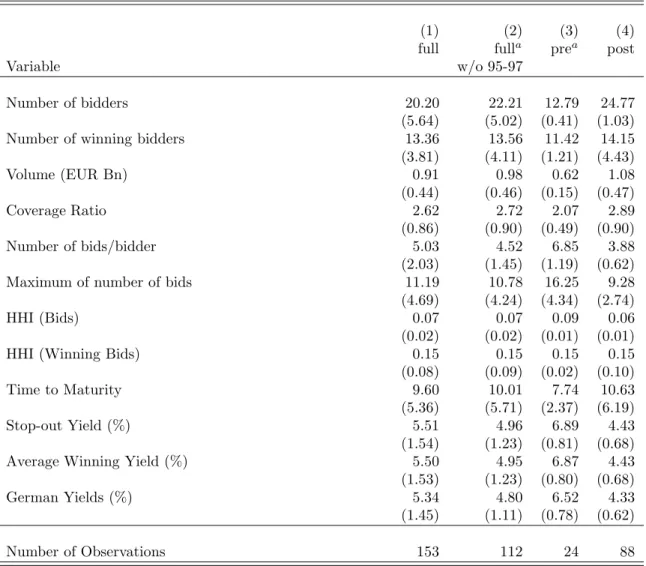
In Table 1 we report summary statistics. In column (1), we report the mean values
and standard deviations of our variables for all auctions. In Column (2), we exclude
auctions from the period 1995 to 1997. These years characterize the transition following
2The reverse is not possible, because with yield tenders only the issue size and maturity were
Figure 1: Development of Government Bond Yields in Europe, 1993-2006
2
4
6
8
10
12
Interest rate
1992m1 1994m1 1996m1 1998m1 2000m1 2002m1 2004m1 2006m1 2008m1 Period
Austria Belgium
Germany Spain
Finland Netherlands
Note: Source ECB.
Austria’s EU accession in 1995 during which the number of bidders steadily increased.
We also exclude the first fourteen auctions, because we could not identify information on
secondary market yields. In Columns (3) and (4), we report the summary statistics for
auctions before 1995 and for auctions after 1997. It can already be seen, that there was
a substantial increase in the number of bidders, and that the average yield in Austria
dropped by 25 basis points more than in Germany (a drop from 6.87 to 4.43 relative to a
drop from 6.52 to 4.33).
2.2
Increase in Bidder Numbers after EU Accession
Austria’s financial markets have become substantially more exposed to competition from
abroad in the context of EU accession in 1995. Only in 1991 capital controls were removed.
By transposing relevant European directives and recommendations into national law, the
”Finanzmarktanpassungsgesetz”, passed in 1993 was instrumental. It contained a new
Table 1: Summary statistics
(1) (2) (3) (4)
full fulla prea post
Variable w/o 95-97
Number of bidders 20.20 22.21 12.79 24.77
(5.64) (5.02) (0.41) (1.03)
Number of winning bidders 13.36 13.56 11.42 14.15
(3.81) (4.11) (1.21) (4.43)
Volume (EUR Bn) 0.91 0.98 0.62 1.08
(0.44) (0.46) (0.15) (0.47)
Coverage Ratio 2.62 2.72 2.07 2.89
(0.86) (0.90) (0.49) (0.90)
Number of bids/bidder 5.03 4.52 6.85 3.88
(2.03) (1.45) (1.19) (0.62)
Maximum of number of bids 11.19 10.78 16.25 9.28
(4.69) (4.24) (4.34) (2.74)
HHI (Bids) 0.07 0.07 0.09 0.06
(0.02) (0.02) (0.01) (0.01)
HHI (Winning Bids) 0.15 0.15 0.15 0.15
(0.08) (0.09) (0.02) (0.10)
Time to Maturity 9.60 10.01 7.74 10.63
(5.36) (5.71) (2.37) (6.19)
Stop-out Yield (%) 5.51 4.96 6.89 4.43
(1.54) (1.23) (0.81) (0.68)
Average Winning Yield (%) 5.50 4.95 6.87 4.43
(1.53) (1.23) (0.80) (0.68)
German Yields (%) 5.34 4.80 6.52 4.33
(1.45) (1.11) (0.78) (0.62)
Number of Observations 153 112 24 88
Note: This table reports the mean values of all our variables. Standard deviations are in parentheses below. Column (1) includes all auctions. Column (2) excludes the transition period 1995 to 1997. Column (3) includes only auctions before 1995 and Column (4) only auctions after 1997. aExcludes first 14 auctions.
service.3 These provisions have resulted in a substantial increased presence of EU based
banks in Austria (with EU subsidiaries holding almost 20% of total bank assets).
From 1991 to 1996 there were between 12 to 15 bidders per auction. Until the end of
1994 only Austrian banks were permitted to bid. EU Common market regulations required
opening participation in the bidding process for all European banks. As a consequence,
the number of bidders increased to an average of almost 25 bidders in the years to follow.
At the end of our sample there were 25 approved bidders, of which only six were Austrian.
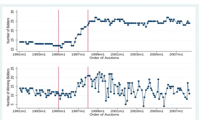
The top panel in Figure 2 shows the evolution of the number of bidders over time.
We plotted a vertical line when Austria joined the European Union in January 1995 and
a second vertical line in January 1998 when the increase in the number of bidders came
to an end. Although the approval of foreign banks started in 1995, we observe a sharp
increase in the number of bidders only later in our sample. The reason for the late increase
is that although in 1995 three foreign banks were admitted some Austrian banks merged.
In 1996, one additional foreign bank was admitted, in 1997, there were nine additional
foreign banks, and in 1998 four additional foreign banks. Afterwards, there were one to
two entrants per year, and some further banks exited due to mergers.4 We thus assume
that the transition process is finished by the end of 1997 and in our further analysis we
drop the observations for the years 1995-1997. The bottom panel in Figure 2 also shows
the number of winning bidders. This number appears to have increased on average, and
so has its variance. After 1997, it rarely happens that all bidders win a positive share in
the auction.
We want to isolate the effect of increased competition and to shed light what may
have happened in the absence of increased bidder numbers. We model the bidding process
with the aim of estimating valuations separately before and after EU accession in the next
section.
3
Model and Estimation
We estimate bidders’ valuations of the auctioned bonds and calculate their surplus. In
this section, we describe the theoretical bidding model and how we estimate bidders’
valuations. We also show the basic estimation results and present evidence on estimated
valuations for the pre-EU period and post-EU period. In Section 4, we then quantify the
effect of competition.
Figure 2: Number of Bidders (top panel) and Winning Bidders (bottom panel)
10
15
20
25
30
Number of Bidders
1991m1 1993m1 1995m1 1997m1 1999m1 2001m1 2003m1 2005m1 2007m1
Order of Auctions
5
10
15
20
25
Number of Winning Bidders
1991m1 1993m1 1995m1 1997m1 1999m1 2001m1 2003m1 2005m1 2007m1
Order of Auctions
Note: Austrian Treasury auctions. Source Oesterreichische Kontrollbank.
3.1
Equilibrium Bidding in Share Auctions
We consider a model of bidding in the spirit of Wilson (1979). We closely follow Kastl
(2011), Horta¸csu and McAdams (2010), and Horta¸csu and Kastl (2012) taking into
ac-count the discreteness of bids.
Auctions. There are T auctions. Each auction t = 1, ..., T is a discriminatory auction of Qt arbitrarily divisible units.
Bidders. There are Nt bidders in auction t. Bidders in each auction are symmetric
and risk-neutral with independent private values (IPV).5
Marginal Valuations. For every auction6, each bidder receives a private signalθ
i drawn
from the distribution F. Signals are distributed independently across bidders as well as
across auctions. The marginal valuation function has the formvi(q, θi). It is increasing in
5The methodology in Kastl (2011) allows for asymmetries by introducingGdifferent groups of bidders
denoted byg such that Nt=P G
g=1N
g
t.Bidders are then assumed to be symmetric only conditional on belonging to groupg. In Section 4, we examine the robustness of our results by allowing for two bidder groups.
θi and weakly decreasing in q.Horta¸csu and Kastl (2012) provide a formal method to test
for the null hypothesis of private values in the Bank of Canada’s three-month treasury-bill
auctions, and do not reject private values in that application. Their test method relies on
the specific institutional setup in the Canadian treasury market, which is not present here.
We do however argue that their results provide support for our assumption of independent
private values in the context of government debt auctions. It can reasonably be argued
that banks have idiosyncratic shocks to their liquidity needs due to deposit flows and the
corresponding reserve requirements. The assumption we impose in our empirical work is
that these shocks are independent conditional on observed macro and secondary market
conditions. In the sequel we drop the index i, as there is no danger of confusion
Gross Utility. Vi(q, θi) =
Rq
0 vi(u, θi)du denotes bidder i’s gross utility when she
re-ceived signal θi and she obtains quantity q.
Action sets. Bidders are required to submit non-increasing bid-schedules bi(.). In
particular, we assume that each bidder’s action set is a triple (bi,qi, Ki) where prices
bi and corresponding cumulative quantities qi are vectors of dimension Ki and Ki is a
finite natural number. We require for 1 ≤ k < Ki that qik < qik+1 and bik > bik+1 and
qik ∈[0,Q¯] where ¯Q≤Q is the maximum quantity bidders are allowed to bid for.
Bid functions. Bidders use pure symmetric strategies. Bidder i’s pure strategy is a mapping from private signals to the set of weakly decreasing bid functions with Ki steps.
A bidder submits a non-decreasing step function yi(p|θi) = PKi
k=1qikI(p ∈ (bik+1, bik]),
where I is the indicator function (note that bik is decreasing in k) and biKi+1 = 0. The
function specifies how much a bidder of type θi demands at price p.
We make two additional assumptions consistent with the auction procedure. First,
we assume that whenever the market clearing price is not unique, the auctioneer uses the
most favorable price from her perspective. Second, bids at the lowest price accepted
(stop-out price) may be subject to pro rata curtailments to provide for a precise representation
of the scheduled issue size.
use interim strategy yi(·|θi) such that the vector y(·|θ) = [y1(·|θ1), . . . , yN(·|θN)] denotes
the vector of submitted bid schedules. Let Qc
i(θ,y(·|θ)) denote the quantity bidder i
obtains given stateθand that bidders are using strategyy(·|θ).Bidderi′sinterim expected
payoffs are given by
Πi(θi) = Eθ−i
Z Qci(θ,y(·|θ))
0
vi(u, θi)du
−
Ki
X
k=1
I(Qci(θ,y(·|θ))> qik)(qik−qik−1)bik
−
Ki
X
k=1
I(qik ≥Qci(θ,y(·|θ))> qik−1)(Qci(θ,y(·|θ))−qik−1)bik, (1)
where qi0 = 0. The first term is the gross-utility the bidder obtains, the second term
is what she pays for quantities on which she is not rationed, and the last term is what
she pays on quantities on which she is rationed. We assume that supply is non-random,
although the OeKB reserves the right to withdraw supply entirely. This happened once
during the sample period, when the yield resulting from the auction exceeded that of
Belgian yields.7
Equilibrium. The equilibrium concept we use is Bayesian Nash equilibrium. A vector of strategies y(·|θ) constitutes a Bayesian Nash equilibrium, if for all bidders i, yi(·|θi)
maximizes her expected utility Πi(θi).
3.2
Estimation of Marginal Valuations
In this section, we describe how we infer the marginal valuations of bidders, vi. Let
Pc(θ,y(·|θ)) denote the market clearing price associated with type vectorθ. Kastl (2012)
7Belgium had historically higher yields because of a considerably higher debt to GDP ratio than
shows that for all steps k but the last step Ki a bidder’s bid function has to satisfy:8
v(qik, θi) =bik+
P r(bik+1 ≥Pc)
P r(bik > Pc > bik+1)
(bik −bik+1) (2)
and at Ki:
biKi =v(¯qi, θi) where ¯qi =supθ−iQ c
i(θi, θ−i,y(·|θ)). (3)
To infer the valuations at the bid steps, we follow the resampling approach proposed
by Horta¸csu and McAdams (2010) and Kastl (2011). The idea is to use observed bid
functions to estimate the distribution of the market clearing pricePc. Since the bid steps
bk are also observed, this allows us to infer marginal valuations v(qik, θi) using (2).
1. We fix bidder iand her bid function yi(p) in auction t.
2. Draw N−1 bid functions with replacement from all bids and compute the residual
supply Q−PN−1
j=1 yj(p).
3. Compute the market clearing pricePcgiven bidderi′sbid functiony
i(p) and whether
bidderi would have won quantity qik at bid bik for all k.
4. Repeat 2.) and 3.) S times. This gives a distribution of market clearing prices for
every bid function yi(p) and hence a estimate of both the numerator and
denomi-nator of the fraction on the right hand side of equation (2).
We perform steps 1 to 4 for every bidder and every auction. In addition, we separate
between the period before 1995 and the period after 1997. Within each period, the bids
are sampled using a four-dimensional kernel including auction-date, issue size, remaining
8Rewriting the first order condition illustrates the trade-off a bidder faces at stepk, equating the cost
and benefit of demanding a lower quantityqik:
P r(bik > Pc> bik+1)(v(qik, θi)−bik) =P r(bik+1≥Pc)(bik−bik+1).
The cost is the loss of surplus (v(qik, θi)−bik) in case the market clearing pricePc is between bik and
maturity, and bidder numbers in the kernel weights.9 We normalize bids by the secondary
market yield of either the auctioned security or a close substitute. We use S = 5000
resamples to estimate the distribution of market clearing prices.
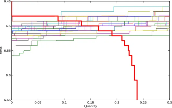
Figure 3 shows 100 randomly drawn residual supply curves and the demand curve of
bidder 35 in auction 21. Since we are considering yield-tenders, we have reversed the
y-axis to be consistent with the exposition of the model. The figure clearly shows that
positive winning probabilities lie within a fairly narrow range.
Figure 3: Bid Function and Random Residual Supplies: Auction 21, Bidder 35
0 0.05 0.1 0.15 0.2 0.25 0.3
6.45
6.5
6.55
6.6
6.65
Quantity
Yields
Note: Own calculations. Source Oesterreichische Kontrollbank.
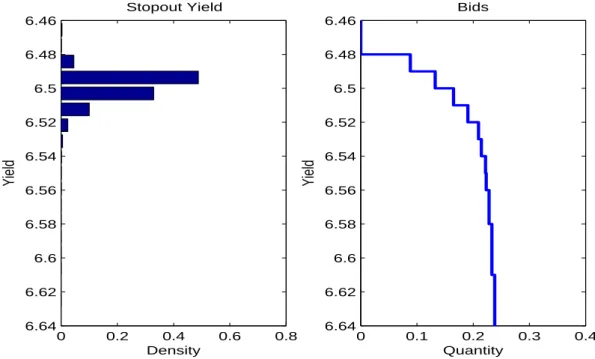
The picture becomes even clearer in Figure 4, which shows that the distribution of the
stop-out price on the left-hand panel has positive density over a range of 10 basis points.
About 90 percent of the mass, however, are over a range of 2 basis points only.
9The bandwidth parameters are set such that for auction t only auctions between t−3 and t+ 3
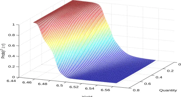
Figure 5 illustrates the estimated probability of winning at a specific quantity-bid
combination. Again, the probability of winning declines very steeply over a very small
range of yields, while for a large range that probability is very close to zero or one.
Figure 6 shows a specific bidder’s bid function and her valuations in auction 21.
Valu-ations for this bidder are up to 4 basis points above her bid. We calculate standard errors
of marginal valuations using a bootstrap. The reported standard errors in the paper are
from a sample of 100 estimates generated by repetitions of the estimation procedure with
a new bootstrap sample of bid functions for the whole sample (see e.g. Table 2).
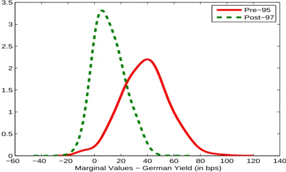
We also present evidence on the estimated valuations for the pre-EU period and
post-EU period. We normalize the valuations by German yields and show them in Figure 7.
We observe a sharp distinction between the two periods and that the difference between
valuations and the German benchmark yield in the latter time period are lower than before
Austria joined the EU. We discuss potential explanations for this shift in valuations once
we have quantified the effect on surplus.
Figure 4: Stop-out Yields, Bids: Auction 21, Bidder 35
6.46
6.48
6.5
6.52
6.54
6.56
6.58
6.6
6.62
6.64
0 0.2 0.4 0.6 0.8
Stopout Yield
Density
Yield
0 0.1 0.2 0.3 0.4
6.46
6.48
6.5
6.52
6.54
6.56
6.58
6.6
6.62
6.64
Quantity
Yield
Bids
Figure 5: Distribution function
0
0.2
0.4
0.6
0.8
6.44 6.46
6.48 6.5
6.52 6.54
6.56 0
0.2 0.4 0.6 0.8 1
Quantity
Yield
Prob(r
c ≥ r)
Note: Own calculations. Source Oesterreichische Kontrollbank.
Figure 6: Bidder valuations: Auction 21, Bidder 35
0 0.05 0.1 0.15 0.2 0.25
6.44
6.46
6.48
6.5
6.52
6.54
6.56
6.58
6.6
6.62
Quantity
Yield
bid
marginal value upper decil median lower decil
Figure 7: Distribution of Bidders’ Valuations pre-EU Period and post-EU Period
−600 −40 −20 0 20 40 60 80 100 120 140
0.5 1 1.5 2 2.5 3 3.5
Marginal Values − German Yield (in bps)
Pre−95 Post−97
Note: Own calculations. Source Oesterreichische Kontrollbank.
4
Quantifying the Effect of Competition
Based on the estimates, we now examine the surplus obtained by bidders in the two
different time periods. Then, we decompose the change in surplus of increased competition
into a strategic effect, due to more aggressive bidding, and a statistical effect, due to
more draws of valuations among bidders. The aim is to quantify the effect of increased
competition following EU accession. Since we cannot actually compute counterfactual
equilibria, we compare auction outcomes under both regimes to a benchmark. To do this,
4.1
Estimating Bidder Surplus
For all auctionst = 1, .., T, we estimate the ex-post surplus Stearned by bidders. Let Qci
be the quantity allocated to bidder i,
St =
Nt
X
i=1
Ki
X
k=1
I(Qci > qik)(qik−qik−1)
+ I(qik ≥Qci(θ,y(·|θ))> qik−1)(Qci(θ,y(·|θ))−qik−1)
·(ˆv(qik)−bik) (4)
and divide this by the issue size Qt to make auctions comparable.
This yields an estimate of the total ex-post surplus earned by bidders in each auction.
To calculate the interim surplus we use the resampling procedure again. For each bidderi
in auctiont, we keep the bid scheduleyi(p|θi) fixed and draw 5000 residual supply curves.
For each of these draws we calculate the surplus using the estimated marginal values.
Finally, we average across the draws to get the interim surplus of bidder iand add up all
the bidders’ surpluses in each auction.
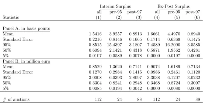
Table 2 reports our estimates of both the interim and ex-post surplus, over the whole
sample period as well as for the periods before and after EU accession. The interim
surplus earned by bidders has dropped by about 3 basis points or 77 percent (see Panel
A). This is a measure in annual yields. Because average time to maturity and average
volume increased after 1997, we also report the respective numbers in million euro in
Panel B. Here we convert the difference between valuation and bid in basis points into the
volume weighted difference between valuation in euro and price paid. According to this
measure the interim surplus dropped from 1.362 to 0.714 million euro or by 48 percent.
The longer maturities and larger volumes thus result in a somewhat smaller proportional
drop in surplus when measured in euro. The results for the ex-post surplus are slightly
more pronounced. Obviously, surplus per bidder, but also surplus per winning bidder,
has declined even more. This is a sharp drop in surplus from a very high level before EU
accession to a level very much in line with other studies (see Kastl (2011)).
Table 2: Interim and Ex-Post Surplus Estimates
Interim Surplus Ex-Post Surplus all pre-95 post-97 all pre-95 post-97
Statistic (1) (2) (3) (4) (5) (6)
Panel A. in basis points
Mean 1.5416 3.9257 0.8913 1.6661 4.4970 0.8940
Standard Error 0.2216 0.8146 0.1665 0.1714 0.6369 0.1475
95% 5.8515 15.4397 3.1807 7.4589 16.2090 3.5585
50% 0.6094 2.1421 0.4318 0.5871 1.9562 0.4281
5% 0.0107 0.0589 0.0078 0.0000 0.0197 0.0000
Panel B. in million euro
Mean 0.8529 1.3620 0.7141 0.9074 1.6189 0.7134
Standard Error 0.1270 0.2984 0.1415 0.0986 0.2461 0.1120
95% 3.0008 6.0393 2.8097 3.3038 6.1207 3.0232
50% 0.3304 0.8241 0.2948 0.3468 0.8724 0.3097
5% 0.0085 0.0194 0.0042 0.0000 0.0080 0.0000
# of auctions 112 24 88 112 24 88
Note: Panel A reports estimates of bidder interim and ex-post surplus as the absolute difference of bids and valuations in basis points. Panel B reports the corresponding volume weighted difference between euro valuation and price paid. Standard errors are calculated using 100 bootstrap replications.
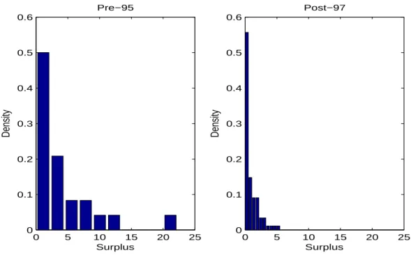
more detailed picture. Even before EU accession most auctions resulted in very small
surplus estimates. However, auctions where large surpluses have been obtained appear
to have become less frequent after EU accession. Overall the variance of outcomes has
been reduced. Figure 8 illustrates the distribution of outcomes as well. It shows that the
increased competition has also stabilized government revenue.
Bidder heterogeneity
One concern with our results might be that the foreign banks that entered the bidding
process after Austria joined the EU are substantially different than Austrian banks. We
therefore relax the symmetry assumption and estimate the interim and ex-post surplus
allowing for two different bidder groups in both periods. We re-estimate the model under
the assumption that banks which participated in both periods draw their valuations from a
Figure 8: Distribution of bidder surplus across auctions
0 5 10 15 20 25
0 0.1 0.2 0.3 0.4 0.5 0.6
Pre−95
Surplus
Density
0 5 10 15 20 25
0 0.1 0.2 0.3 0.4 0.5 0.6
Post−97
Surplus
Density
Note: Own calculations. Source Oesterreichische Kontrollbank.
that participated only after EU accession could be labeled international competitors. We
report the estimation results in the Appendix (Table A.1). We estimate an interim surplus
of 3.8735 basis points in the first period and of 0.8789 basis points in the second period.
These values are very close to the estimated interim surplus under symmetry (3.9257
and 0.8913 basis points). Our results appear to be extremely robust. Consequently, we
maintain the symmetry assumption.
Comparison with Reduced Form Evidence
We now compare our results from the structural model to the results from
difference-in-difference regressions. We compare Austrian and German government bonds and assume
that the yields of German government bonds were not affected by Austria joining the EU.
As Austria is a small country about a tenth of the size and population of Germany, we
consider that this assumption is not too strong. The German bonds are selected so that
they are similar to the Austrian bonds with respect to their maturity. We then regress
one for auctions after 1997 and an interaction between these two dummy variables. The
interaction may measure the effect of increased competition. To control for other
de-terminants, we also include the maturity of the bonds, inflation, GDP growth, a time
trend as well as the interaction of the time trend with auctions after 1997 in our
regres-sions. To account for serial correlation, we include an autoregressive term of order one
(Bertrand et al., 2004). We report the results of the difference-in-difference regressions in
the Appendix (Table A.2). We find that the estimated effect of increased competition on
Austrian government bonds is -0.511 percentage points.
This is a rather strong effect compared to the results from our structural analysis. The
gap can be explained by the accompanied change in valuations that occurred between
the two time periods, as documented in Figure 7. Valuations for Austrian treasuries
increased after EU accession (yields have dropped) relative to German bonds. The modes
of the two distributions are roughly 35 basis points apart, explaining a larger part of
this gap. Presumably, Austrian bonds became more liquid and substitutable to other
European bonds. For instance, only 30%10 of Austrian sovereign debt was held by foreign
institutions in 1995. This number increased to 80% by 2008.11
Isolating the Statistical Effect
We want to quantify to what extent the competitive effect is really due to more aggressive
bidding. Increasing the number of bidders also results in an increase in the number of
draws of valuations. Hence, even without more aggressive bidding there would be a
change in surplus, simply because extreme draws from the distribution of valuations
would become more likely.12
After Austria joined the EU, the number of bidders has increased on average by eleven,
10Annual Report of the Austrian Fiscal Advisory Council. 11ECB, Statistical Data Warehouse.
12This is readily illustrated in a first price sealed bid auction with independent private valuesθ
idrawn from Uniform[0, 1]. Suppose we wish to consider an increase in the number of bidders fromN1 to N2.
The expected surplus of each bidder changes from N 1
1(N1+1) to 1
N2(N2+1). Now, suppose that there are
actually N2 bidders but they bid as if they were onlyN1 bidders. In this case the expected surplus of
each bidder would be N1(N12+1). A fraction of
N2
from roughly 13 bidders to an average of more than 24 bidders. To calculate the
statis-tical effect for auctions before EU accession, we thus perform the following experiment,
employing again a resampling procedure similar to the one used in estimating marginal
values. For each bidder iand each auctiont, we fix her demand. We randomly draw with
replacement Nt −1 + 11 observed demand curves and compute bidder i’s surplus. We
average this surplus acrossS = 5000 resamples. Summing over all bidders’ surpluses gives
an estimate of the surplus in auctiont. The difference between the actual surplus earned
and the surplus under the counterfactual with eleven more bidders is a pure statistical
effect of increasing bidder numbers, as it ignores that bidding behavior will also change
in response to increased bidder numbers. We also perform the corresponding experiment
reducing the number of bidders by eleven for the period following EU accession. Figure
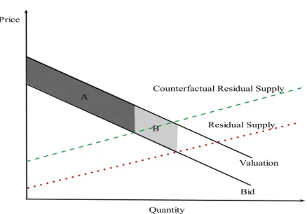
9 illustrates this statistical effect.
Figure 9: Statistical effect
For illustrative purposes, we use linear bid functions and assume that a change in the
number of bidders only affects the intercepts and not the slopes of the residual supply
function. When there are only 13 firms, the market clearing price is given by the
intersec-tion of a bidder’s demand funcintersec-tion and the residual supply (dotted line). Since this is a
B. Now increasing the number of bidders results in a reduced residual supply given by
the dashed line, causing a higher equilibrium stop-out price (lower yield) and the bidder
winning a lower quantity. Its surplus is given the by the dark grey area A only. The
reduction in surplus due to the statistical effect is thus given by the light grey areaB.
Table 3 presents the results. Columns (1) and (2) illustrate the effect of increasing
the actual number of bidders in each pre-95 auction by eleven. In Panel A, we find that
just increasing bidder numbers without changing strategic behaviour before 1995 would
reduce surplus by roughly 63 percent (going from 3.9257 basis points to 1.4707 basis
points). Panel B provides the effect of increasing competition in bidder surplus in million
euro. Increasing the number of bidders decreases their surplus by 64% (going from 1.362
to 0.497 million euro). Columns (3) and (4) illustrate the effect of reducing the number of
bidders in the post-97 auctions by eleven. Reducing bidder numbers by eleven after 1997
would increase surplus in basis points (in million euro) by 45 (41) percent. Hence, the
strategic effect through more aggressive bidding appears to account for a large fraction of
the estimated change in surplus.
4.2
Evaluation of auction mechanism and allocative efficiency
Finally, we examine how increased competition has affected the efficiency of the auction
mechanism. We ask how the discriminatory auction performs in terms of revenue (interest
paid and funds raised) and surplus (left to bidders) relative to the widespread alternative
mechanism, namely a uniform auction. As in a discriminatory auction, the uniform
auction aggregates bids to find the market clearing price, but bidders pay the market
clearing price for all units they purchase. Whether a discriminatory auction is superior
to a uniform auction has been a long standing debate in the literature. Theoretically,
these auction formats cannot be ranked (see e.g. Ausubel et al. (2015)) and it therefore
becomes an empirical question. While we cannot solve for the equilibrium strategies in a
uniform auction, we consider a hypothetical uniform price auction with truthful bidding
Table 3: Interim and Counterfactual Surplus Estimates
Increasing Decreasing bidder # pre-95 bidder # post-97
counter- counter-actual factual actual factual
Statistic (1) (2) (3) (4)
Panel A. in basis points
Mean 3.9257 1.4707 0.8913 1.2934
Standard Error 0.8146 0.4326 0.1665 0.1929
95% 15.4397 7.1853 3.1807 4.3179
50% 2.1421 0.3269 0.4318 0.7204
5% 0.0589 0.0029 0.0078 0.0527
Panel B. in million euro
Mean 1.3620 0.4970 0.7141 1.0099
Standard Error 0.2984 0.1632 0.1415 0.1555
95% 6.0393 2.4361 2.8097 3.3673
50% 0.8241 0.1409 0.2948 0.4024
5% 0.0194 0.0011 0.0042 0.0304
# of auctions 24 24 88 88
# of bidders 12.79 23.79 24.77 13.77
# of winning bidders 9.62 13.33 12.54 10.15
Note: Panel A reports interim and counterfactual surplus as the absolute difference of bids and valuations in basis points. Panel B reports the corresponding volume weighted difference between euro valuation and price paid. Columns (1) and (2) illustrate the effect of increasing the number of bidders in the pre-95 auctions by eleven assuming bidding behaviour remains the same. Columns (3) and (4) illustrate the effect of reducing the number of bidders in the post-97 auctions by eleven assuming bidding behaviour remains the same. Standard errors are calculated using 100 bootstrap replications.
(2010).13
Table 4 shows the difference in performance between the hypothetical uniform auction
and the discriminatory auction, both in terms of interest rates (basis points) and revenue
(million euro). Panel A illustrates the performance from the government’s perspective,
i.e. a reduction in basis points is a favorable result for the government, corresponding to
increased revenue in euros. Overall the hypothetical uniform auction does not perform
13Kastl (2011) shows that when bidders are constrained in the number of steps they bid, bidders may
submit bids above their marginal valuations (in our case demand even lower interest on the government bonds). To provide a more conservative evaluation of the relative efficiency of the discriminatory auction, we also consider a hypothetical uniform auction where bidders bidvkat stepk+ 1. As this is not defined at the first step, we assume that the first bid isb1=v1+ (v1−v2). This results in even lower equilibrium
significantly better in terms of revenue (interest paid in terms of basis points).14
How-ever, Panel A also shows that before 1995, the hypothetical uniform would have saved
the government 1.6274 basis points (or increased its revenue by 0.46 million euro).
Af-ter 1997, the difference becomes significantly negative indicating an advantage for the
discriminatory auction.
Table 4: Auction mechanism
in basis points in Mill. euro all pre-95 post-97 all pre-95 post-97
Statistic (1) (2) (3) (4) (5) (6)
Panel A. Revenue difference
Mean -0.1593 -1.6274 0.2411 -0.0876 0.4595 -0.2368
Standard Error 0.1763 0.7479 0.0601 0.0690 0.2425 0.0472
95% -3.2532 -14.0865 -0.5688 -1.3638 -1.1548 -1.4074
50% 0.2501 0.2723 0.2474 -0.1408 -0.0849 -0.1617
5% 1.5009 2.6721 1.2847 1.3042 4.1436 0.3694
Panel B. Surplus difference
Mean 0.4168 0.0208 0.5248 0.3563 0.0367 0.4435
Standard Error 0.1547 0.6141 0.0836 0.0666 0.2062 0.0597
95% 2.0560 5.6938 1.5197 1.4675 2.3011 1.4493
50% 0.4379 0.4077 0.4400 0.2874 0.1164 0.3120
5% -2.1596 -7.6804 0.0110 -0.7827 -2.9451 0.0217
# of auctions 112 24 88 112 24 88
Note: This table reports the difference in performance between the hypothetical uniform auction and the discriminatory auction. Panel A reports the effect on government revenue; Panel B reports the effect on bidders’ surplus. In columns (1) (3), we report the difference in basis points, while columns (4) -(6) show the difference in million euro valuation and price paid. Surplus in basis points is the absolute difference of yield bid and valuation. Surplus in euro is the corresponding volume weighted difference between euro valuation and price paid. Standard errors are calculated using 100 bootstrap replications.
Panel B illustrates the effects of the alternative auction format on bidder surplus.
The uniform auction leaves bidders a .4168 basis points higher surplus on average over
the sample period. The difference in surplus is even larger under increased competition
than before 1995. It may at first be surprising that the hypothetical uniform auction
14Overall revenue differences are negative both in basis points and euro (Columns 1 and 4), which
can improve both revenue for the government and increase bidders surplus as it is the
case for the period before 1995. The reason is that under limited competition before EU
accession bidders were regularly shading bids even below the market clearing price heavily.
This leads to a re-allocation of shares to bidders with high valuations but bids below the
clearing price in the discriminatory auction. Bidders’ surplus increases, as they only pay
the uniform price rather than their bid on inframarginal units won. The government
benefits from the higher market clearing price. After EU accession increased competition
results in bidders shading much less around the market clearing price. This limits the
scope for improving efficiency through re-allocating units to bidders with high valuations
at marginal units. Moving to a uniform price has a smaller effect on the market clearing
price. While bidders benefit from a lower price on the inframarginal units, this results in
a loss in revenue for the government.
We finally look at the allocative efficiency of the discriminatory auction mechanism
by re-allocating the shares won to the highest inferred valuations. That is, we re-arrange
quantity bids by sorting them according to our estimates of marginal valuations (as the
hypothetical uniform would do). The results are reported in columns (1)-(3) of Table
5. We find that this mechanism would on average reallocate 16% of quantities won.
This amount seems substantial at first and does not change significantly with increased
competition. We then look at the value weighted reallocated share of total surplus, and
calculate the percentage change in efficiency due to the discriminatory auction in percent.
The results are reported in columns (4)-(6) of Table 5. We see that the efficiency increase
from truthful bidding is very small, 0.09% before 1995, and 0.02% after 1997. Our results
for the post 1997 period are comparable to Horta¸csu and McAdams (2010), who report a
value of about 0.02%. If we add the changes in bidders’ surplus and revenues as reported
in Table 4, we see that the efficiency loss equals on average 500,000 euro per auction
Table 5: Allocative efficiency and total surplus
Allocation Total surplus
in percent
all pre-95 post-97 all pre-95 post-97
Statistic (1) (2) (3) (4) (5) (5)
Mean 15.5835 17.6786 15.0122 0.0368 0.0941 0.0212
Standard Error 0.8944 1.7728 0.9402 0.0054 0.0161 0.0054
95% 42.8944 47.6964 41.2075 0.1794 0.5504 0.0804
50% 12.7119 13.5232 11.5499 0.0069 0.0224 0.0053
5% 0.0000 1.0660 0.0000 0.0000 0.0003 0.0000
# of auctions 112 24 88 112 24 88
Note: This table reports the percentage difference in allocation (columns (1) - (3)) and total surplus between the hypothetical uniform auction and the discriminatory auction (columns (4) - (6)). Standard errors are calculated using 100 bootstrap replications.
5
Conclusions
We use recently developed methods to estimate bidders’ marginal values for the bonds
purchased. Knowledge of the marginal valuations allows us to quantify the effect of
in-creased competition on bidder surplus. We find that overall surplus decreases significantly,
but by a much smaller amount than what reduced form regressions would have suggested.
A shift in the distribution of marginal valuations indicates that Austrian bonds have also
become a more attractive product due to increased liquidity and substitutability. This
is mirrored by the fact that the share of Austrian sovereign debt held by foreign
institu-tions increased by 50 percentage points between 1995 and 2008. The change in surplus
itself appears to be largely due to more aggressive bidding. We also find that while
un-der limited competition before EU accession a change in the auction format may have
improved surplus extraction and efficiency, under increased competition the question of
References
Ausubel, L. M., Cramton, P., Rostek, M., and Weretka, M. (2015). Demand reduction
and inefficiency in multi-unit auctions. Review of Economic Studies, 81(4):1366–1400.
Bertrand, M., Duflo, E., and Mullainathan, S. (2004). How much should we trust
differences-in-differences estimates? The Quarterly Journal of Economics, 119(1):249– 275.
Black, S. E., Devereux, P. J., and Salvanes, K. G. (2008). Staying in the classroom and
out of the maternity ward? the effect of compulsory schooling laws on teenage births.
The Economic Journal, 118(530):1025–1054.
Bresnahan, T. F. and Reiss, P. C. (1991). Entry and competition in concentrated markets.
Journal of Political Economy, 5:977–1009.
Elsinger, H. and Zulehner, C. (2007). Bidding behavior in Austrian treasury bond
auc-tions. Monetary Policy and the Economy, 2:109–125.
Fevrier, P., Preget, R., and Visser, M. (2004). Econometrics of share auctions. mimeo,
CREST.
Fort, M., Schneeweis, N., and Winter-Ebmer, R. (2011). More schooling, more children:
Compulsory schooling reforms and fertility in europe. Working Paper No 1111, The
Austrian Center for Labor Economics and the Analysis of the Welfare State.
Horta¸csu, A. and Kastl, J. (2012). Valuing dealers’ informational advantage: A study of
Canadian treasury auctions. Econometrica, 80(6):2511–2542.
Horta¸csu, A. and McAdams, D. (2010). Mechanism choice and strategic bidding in
di-visible good auctions: An empirical analysis of the Turkish treasury auction market.
Huck, S., Normann, H.-T., and Oechssler, J. (2004). Two are few and four are many:
Number effects in experimental oligopolies. Journal of Economic Behavior &
Organi-zation, 53(4):435–446.
Kastl, J. (2011). Discrete bids and empirical inference in divisible good auctions. The
Review of Economic Studies, 78(3):974–1014.
Kastl, J. (2012). On the properties of equilibria in private value divisible good auctions
with constrained bidding. Journal of Mathematical Economics, 48(6):339–352.
Selten, R. (1973). A simple model of imperfect competition, where 4 are few and 6 are
many. International Journal of Game Theory, 2(1):141–201.
Waschiczek, W. (2005). The impact of EU accession on Austria’s financial structure.
Monetary Policy and the Economy, 2:117–129.
Weiss, L. W. (1989). Concentration and price. MIT Press Cambridge, MA.
A
Appendix: Results with two bidder groups
The method illustrated by Kastl (2011) allows for bidder heterogeneity. We drop the
assumption of homogeneity, assume two groups in each period, and estimate the interim
and ex-post surplus. Before 1995, the first group of banks consists of those that dropped
out after the 56-th auction which is in the transition period and the second group consists
of the remaining banks. After 1997, the first group of banks consists of those that joined
after the 56-th auction and the second group consists again of the remaining banks. Note,
we cannot identify banks and thus we cannot define Austrian and foreign banks. We thus
tried various cutoff points between the 38-th and 66-th auction. We chose the 56th auction
as immediately after this auction, there is a sharp increase in the number of bidders. The
results shown in Table A.1 are however robust to the choice of the cut-off point.
Table A.1: Interim and Ex-Post Surplus Estimates with Two Bidder Groups
Interim Surplus Ex-Post Surplus all pre-95 post-97 all pre-95 post-97
Statistic (1) (2) (3) (4) (5) (6)
Panel A. in basis points
Mean 1.5206 3.8735 0.8789 1.6405 4.4014 0.8875
Standard Error 0.1935 0.7799 0.1337 0.1588 0.6446 0.1123
95% 5.8350 15.5936 3.2202 7.3397 16.0945 4.0506
50% 0.5656 2.1413 0.4081 0.5248 2.1537 0.3863
5% 0.0099 0.0555 0.0072 0.0000 0.0112 0.0000
Panel B. in million euro
Mean 0.8510 1.4140 0.7736 0.9068 1.6748 0.7765
Standard Error 0.0628 0.2742 0.1392 0.0635 0.2588 0.1107
95% 2.8344 5.9552 2.6876 3.1945 6.1652 3.1376
50% 0.3315 1.0322 0.2853 0.3470 0.9977 0.2939
5% 0.0080 0.0198 0.0042 0.0000 0.0082 0.0000
# of auctions 112 24 88 112 24 88
B
Appendix: Reduced Form Evidence
In Table A.2, we report the difference-in-difference regression results in more detail. In
Column (1), we report the results of our basic specification. The time trend is negative
indicating that yields have decreased over the years, while the time trend after the year
1997 is positive indicating that yields decline in a less pronounced way. We also observe
that the yields of Austrian government bonds are on average 0.441 percentage points
(44.1 basis points) higher than the yields of German government bonds. The yields of all
government bonds are by 2.021 percentage points lower after joining the EU. The
esti-mated effect of increased competition on Austrian government bonds is -0.511 percentage
points. This is a rather strong effect. We observe that maturity, inflation rate and GDP
growth carry the expected signs. A longer maturity is associated with higher yields, i.e.,
an increase in the maturity of a bond by one year increases the yield by 0.038 percentage
points. GDP growth and inflation also have a positive effect on yields. When inflation
increases by one percent, the yields increase by 0.155 percent, whereas when GDP grows
by one percent, the yields increase by 0.110 percent. The estimate of the AR(1) term is
equal to 0.832 and significantly different from zero.15
We next examine the robustness regarding the definition of the transition period. In
Column (2), we assume that the transition process was already finalized in the year
1996. None of our results change significantly. The estimated effect of the increased
competition on Austrian government bonds is -0.498, only slightly larger than in our
preferred specification. In Columns (3) and (4), we present the robustness of our estimates
to placebo treatments. We might be concerned that the increase in bidder numbers picks
up some additional unspecified time effect in Austria or Germany. In particular, we are
concerned about the general convergence of interest rates in the euro area at the time.
To test for this, we use placebo treatments. Similar to Black et al. (2008) and Fort et al.
(2011), we introduce such a treatment and add an hypothetical increase in competition
before and after Austria actually joined the EU. These placebo reforms should not have
Table A.2: Difference-in-difference results
Variable (1) (2) (3) (4)
Constant 7.059 7.062 7.088 7.458
(0.201) (0.201) (0.219) (0.189)
Maturity 0.038 0.041 0.039 0.040
(0.004) (0.004) (0.004) (0.004)
Inflation Rate 0.155 0.151 0.173 0.080
(0.032) (0.031) (0.033) (0.030)
GDP Growth 0.110 0.108 0.102 0.096
(0.017) (0.017) (0.018) (0.015)
Time trend -0.053 -0.053 -0.061 -0.057
(0.004) (0.004) (0.007) (0.004) Time trend×Auctions after Austria joining EU 0.040 0.038 0.048 0.059 (0.004) (0.004) (0.007) (0.004)
Austria 0.441 0.438 0.439 0.400
(0.076) (0.079) (0.095) (0.069) Auctions after Austria joining EU -2.021 -1.831 -2.262 -3.638 (0.211) (0.197) (0.290) (0.253) Auctions after Austria joining EU×Austria -0.511 -0.498 -0.537 -0.403 (0.096) (0.097) (0.140) (0.098)
Auctions after Placebo Date 0.225 -1.001
(0.173) (0.101)
Placebo Date×Austria 0.028 -0.061
(0.163) (0.087)
AR(1) 0.832 0.815 0.830 0.839
(0.039) (0.039) (0.039) (0.037)
Observations 250 266 250 250
Adjusted R-squared 0.96 0.95 0.96 0.97
Note: The dependent variable is the yield of Austrian and German government bonds. Placebo dates are February 8, 1994 in Column (3) and April 6, 2004 in Column (4). In Column (2) we assume that the transition process was already finalized at the end of 1996. In all other columns, it is the year 1997. Consequently there are more observations in (2). Standard errors are shown in parentheses below the estimated coefficients.
had any impact on Austrian government bonds. If we find an impact, our results might
be driven by other unobserved mechanisms. Adding placebos before (Column 3) and after
Austria joined the EU (Column 4) slightly alter the estimates of the original treatment,