本文 Thesis 総合研究大学院大学学術情報リポジトリ A1857本文

(1)

Short-distance correlation functions and non-

perturbative renormalization of quark

currents in lattice QCD

Masaaki TOMII

Doctor of Philosophy

Department of Particle and Nuclear Physics

School of High Energy Accelerator Science

SOKENDAI (The Graduate University for

Advanced Studies)

定

(2)

(3)

SOKENDAI

(T ^HE G ^RADUATE U NIVERSITY FOR _A DVANCED _S TUDIES ₎

D

^OCTORAL

T

^HESIS

Short-distance correlation functions and

non-perturbative renormalization of quark

currents in lattice QCD

Author:

Masaaki TOMII

Supervisor: Prof. Shoji HASHIMOTO

A thesis submitted in fulfillment of the requirements for the degree of Doctor of Philosophy

in the

School of High Energy Accelerator Science Department or Particle and Nuclear Physics

(4)

(5)

iii

Abstract

Short-distance correlation functions and non-perturbative renormalization of quark currents in lattice QCD

by Masaaki TOMII

Precise predictions of the Standard Model (SM) are important for the search of new physics. Precision of the SM predictions needs to be improved for comparisons with forthcoming experiments. Uncertainty of the SM predictions mainly arises from the contribution of Quantum Chromodynamics (QCD), which is the theory of strong interaction of quarks, anti-quarks and gluons. This is because QCD cannot be treated by perturbation theory at low energies and the parameters of QCD such as the strong coupling constant have large uncertainty compared to other SM parameters.

Correlation functions of quark currents provide a rich source of information on the QCD vacuum at various scales ranging from perturbative to non-perturbative regions. At short distances, they become mostly perturbative due to the asymptotic freedom of QCD. Using high order perturbation theory, they can be used to determine the strong coupling constant. At long distances, on the other hand, the correlation functions carry the information about hadron spec- trum and the low energy constants of QCD, which are the parameters in the chiral perturbation theory.

Correlation functions can be calculated from first principles using lattice QCD. In lattice QCD, the spacetime is discretized and compactified with some boundary conditions. Then, the degrees of freedom of the system in lattice QCD become finite and numerical path integral is feasible using the Monte Carlo method. Taking the infinite volume limit and the continuum limit for the correlation functions on the lattice, one can obtain the correlation functions in the continuum.

Comparison of the correlation functions in the continuum theory and on the lattice may determine fundamental quantities of QCD. In fact, lattice QCD is usually applied to calculate hadron masses and decay constants from the correlation functions at long distances. Similarly, the comparison at short distances can in principle provide a determination of the strong coupling constant. The comparison at short distances needs to be performed after eliminating lattice artifacts. The lattice calculation at short distances suffers from unphysical discretization effect which becomes more significant as the distance becomes small. A careful investigation of the discretization effect is, therefore, necessary for the precise determination of the strong coupling constant.

(6)

In this thesis, we analyze short-distance correlation functions both on the lattice and in the continuum, and investigate the region where the lattice results agree with the continuum theory after removing the lattice artifact. The lattice simulation is carried out on 14 gauge field ensembles generated by the JLQCD collaboration. The ensembles contain 2 + 1 flavors of sea quarks described by the Möbius domain-wall fermions, which realize precise chiral symmetry on the lattice. The pion masses on these ensembles are in the region 220–500 MeV. The lattice spacings are 0.044 fm, 0.055 fm, and 0.080 fm. We subtract the discretization effects within the mean field approximation. We extrapolate lattice results to the physical pion mass and the continuum limit.

Vector, axial-vector, scalar, pseudoscalar channels of the correlation functions in perturbation theory are available to the four-loop level. Using such well-advanced results, we investigate the convergence property of perturbative expansions. Slight deviation of the correlation functions at short distances from those in perturbation theory is explained by the Operator Product Expansion (OPE), which accommodates some non-perturbative effects in the correlation functions by expanding a product of operators into a series of composite operators.

We utilize the correspondence of continuum and lattice correlation functions for the renormalization of quark currents. It turns out that although the correlation functions on our lattice ensembles suffer from significant discretization effect in the perturbative region, the analysis including OPE allows us to determine the renormalization constants at slightly longer distances, where the discretization effects is well-managed. We obtain the renormalization constants of the vector current and the scalar density with the precision of O(1%) or less.

Using the result of the renormalization, we test the consistency between the correlation functions on the lattice and experiments. We calculate the vector and axial-vector correlation functions from the experimental results of spectral functions obtained through the hadronic tau decays by the ALEPH collaboration. We verify that the experimental correlation functions are in good agreement with our lattice results.

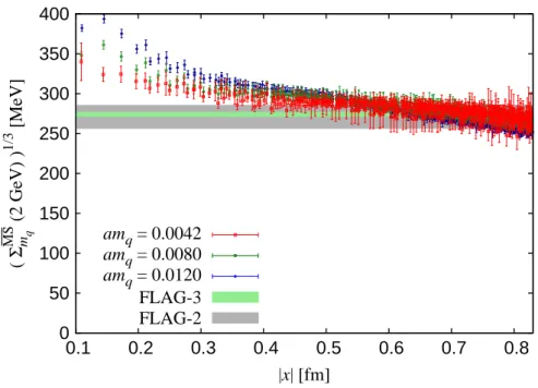
The result of the renormalization is also applied to an analysis of the chiral condensate, which is an order parameter of the spontaneous breaking of chiral symmetry in QCD and plays an important role in the chiral perturbation theory. We extract the chiral condensate from current correlators in the OPE regime. This result agrees with the world average of lattice calculation of 2 + 1 flavors QCD.

(7)

v

Acknowledgements

First of all, I express my deep gratitude to Prof. Shoji Hashimoto, my supervisor, for his great advices, continuous regards, and many important discussions for three years even though he has been very busy with a hectic schedule. With out his supports, I could not have studied so far.

I also thank M. Hayakawa for teaching me a lot of important things as a researcher and showing me his attractive passion. I appreciate H. Matsufuru and T. Kaneko’s effort to secure large disk storages /xwork** and to create my account on the workstations scdl360d.kek.jp and scbc2fe.kek.jp. This study is done in the JLQCD collaboration. I thank H. Fukaya, J. Noaki, G. Cossu, B. Fahy, and all other JLQCD members for many discussion, comments, and teachings. I could have discussions with other professional researchers, F. Knechtli, P. Boyle, T. Izubuchi, C. Lehner, and H. Ohki, and many researchers in KEK. I thank all of these people.

My research activity is successful in virtue of several supportive programs and related peole. My trips to JPS meetings, lattice conferences and other workshops are aided by the Student Travel Reimbursement program managed by SOKENDAI and SH’s grant, the Grant-in-Aid of the Japanese of Educations No. 26247043. The trip to BNL is aided by The Short-Stay Abroad Program managed by SOKENDAI. I thank M. Oishi, a secretary of the lattice group in KEK Theory Center, and members of Postgraduate Education Unit in KEK for their help with the procedures for these trips. I was employed by KEK as a research assistant (RA). Numerical simulations are carried out on Hitachi SR 16000 and IBM System Blue Gene/Q (BGQ) at KEK under a support of its Large Scale Simulation Program (Nos. 13/14-04,14/15-10). The JLQCD collaboration thanks PB for the optimized code for BGQ.

Finally, I am grateful to my family for continuous encouragement and supports.

Masaaki Tomii

(8)

(9)

vii

List of Figures

1.1 A sketch of current correlators. . . 2 2.1 Perturbative expansion of the vector correlator calculated with the coupling con-

stant as(1/|x|). . . 11 2.2 Perturbative expansion of the vector correlator calculated with the coupling con-

stant as^(µ^BLMx ). . . 11 2.3 View of the convergence of the perturbative expansion of the vector correlator at

|x| = 0.2, 0.3, 0.4, 0.5 fm as functions of the scale µ^∗xof the coupling constant. . . 12 2.4 Perturbative expansion of the vector correlator calculated with the coupling con-

stant as^(µ^∗,optx ) at the optimized scale. . . 13 2.5 Scalar correlator renormalized at 1/|x| in the MS scheme calculated by a pertur-

bative series of as(1/|x|). . . 15 2.6 Scalar correlator renormalized at 2 GeV in the MS scheme calculated by a pertur-

bative series of as(1/|x|). . . 15 2.7 Scalar correlator renormalized at 2 GeV in the MS scheme at the four-loop level

at|x| = 0.2, 0.3, 0.4, 0.5 fm as functions of µ^∗x^{and µ}^′x^. . . . 16 2.8 View of the convergence of the perturbative expansion of the scalar correlator

renormalized at 2 GeV in the MS scheme at|x| = 0.2, 0.3, 0.4, 0.46 fm as functions of the scale µ^∗_xof the coupling constant. . . 17 2.9 Scalar correlator renormalized at 2 GeV in the MS scheme calculated with the

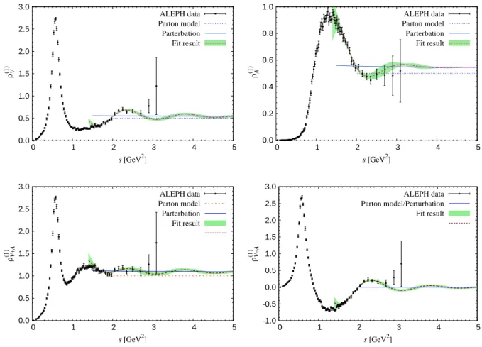
optimized scales µ^′_x= µ^{′ opt}_x and µ^∗_x= µ^∗,opt_x . . . 18 2.10 Spectral functions measured by the ALEPH collaboration for four channels

V, A, V + A, V − A plotted with the fit result based on the resonance model. ^{. .} ²⁷ 2.11 Vector and axial-vector correlators calculated from the ALEPH spectral functions,

perturbation theory, and resonance based model. . . 29 2.12 Decomposition of the contribution of the spectral function to the vector correla-

tor. . . 30 2.13 Decomposition of the contribution of the spectral function to the axial-vector cor-

relator. . . 30 3.1 Pseudoscalar correlator without reducing the discretization effect, plotted with

the corresponding mean field approximation and its asymptotic behavior in the long distance limit. . . 36

(12)

3.2 Pseudoscalar correlator after subtracting the discretization effect in the mean

field level. . . 36

3.3 Separation of the pseudoscalar correlator into four regions of θ. . . 38

3.4 Same as Fig. 3.3 but for the vector channel. . . 38

3.5 Detailed view of Fig. 3.4 in 0^◦ ≤ θ < 20^◦^{and 20}^◦ ≤ θ < 30^◦^. . . . 39

3.6 Pseudoscalar and vector correlators divided by the tree level continuum correlator after applying the tree level correction by the multiplicative manner. . . 40

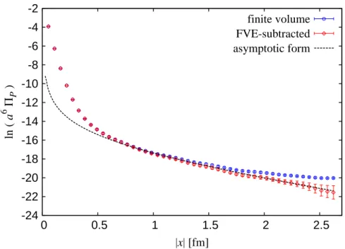
3.7 Pseudoscalar correlator in the time-direction (|x| = t) before and after subtracting the finite volume effects, plotted with the asymptotic form (3.12) in the long distance limit. . . 41

3.8 Pseudoscalar correlator before and after subtracting the finite volume effects. . . 42

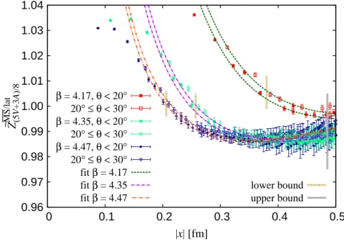
4.1 ^Z^e_V^MS/lat(a; x) and eZ_A^MS/lat(a; x) at three different input masses. . . 48

4.2 Z^e_{(5V +3A)/8}^MS/lat (a; x) calculated on the same ensembles as in Fig. 4.1. . . 48

4.3 Z^e_{(5V +3A)/8}^MS/lat (a; x) at three different lattice spacing with Mπ ∼ 300 MeV. . . ⁴⁹

4.4 ^Z^e(S+P )/2+(V −A)/16^MS (2 GeV, a; x) at three different lattice spacing with Mπ ∼ 300 MeV. . . . 52

5.1 R_{V +A}calculated at the same ensembles as in Fig. 4.2, plotted with the prediction of perturbation theory (dashed curve) and the result of the experiment (bands). 54 5.2 Same as Fig. 5.1 but calculated at the same ensembles as in Fig. 4.1. . . 54

5.3 Extrapolation of RV +Ato the physical point. . . 55

5.4 RV −A calculated at the same ensembles as in Fig. 4.2, plotted with result of the experiment with (hatched band) and without the duality violating term. . . 57

5.5 Same as Fig. 5.4 but calculated at the same ensembles as in Fig. 4.1. . . 57

5.6 Extrapolation of RV −Ato the physical point. . . 58

5.7 Chiral condensate calculated from the vector and axial-vector correlator at the same ensembles as in Fig. 4.1. . . 60

5.8 Same as Fig. 5.7 but the result at the same ensembles as in Fig. 4.3. . . 60

A.1 Wick’s rotation from the Minkowski to the Euclidean space in the momentum and coordinate spaces. . . 67

F.1 Same as Fig. 3.3 but for the scalar and axial-vector channels. . . 99

F.2 Z^e_S(x), eZ_P(x) and some combinations of them. . . 100

F.3 Same as Fig. 4.3 but the results at other ensembles. . . 101

(13)

xi

List of Tables

2.1 Some relations between the momentum formula and the coordinate formula through

Fourier transforms. . . 21

3.1 Lattice ensembles used in this work. . . 35

4.1 Result for the renormalization factor of the vector channel. . . 50

4.2 Result for the renormalization factor of the scalor channel. . . 52

5.1 Chiral condensate extracted from the global fit. . . 61

(14)

(15)

1

Chapter 1

Introduction

The Standard Model (SM) of elementary particles forms the basis for the progress in high energy physics. It describes the fundamental particles and their interactions. The formulation of the SM is completed in the 1970s and its validity has been supported by a lot of experiments. At the same time, several experiments have shown small but significant deviations from the SM, which can be understood as signs of new physics beyond the SM. Since these signs must play a key role in the progress in high energy physics, many high energy physicists concentrate their effort on testing the SM.

Recent activities of experimentalists aim at the SM tests by a drastic improvement in the precision in the next decade. For example, Belle II experiment is going to quantify the effects of CP violation focusing on the decay processes of B mesons. The groups at J-PARC and Fer- milab are going to measure the muon anomalous magnetic moment, which may show a sign of new physics, with the precision five times better than the previous experiment at BNL. These experiments are expected to produce results in early 2020s.

On the theory side, researchers are trying to provide SM predictions with the precision which competes with that of the forthcoming experiments. As well known, precise calculations of the contribution of Quantum Chromodynamics (QCD) is the most difficult part in such efforts. The crucial origin of this difficulty is the spontaneous breaking of chiral symmetry in the QCD vacuum. At low energies (≲ 1 GeV), perturbation theory is no longer valid and there are a lot of unpredictable effects such as instanton interactions. At high energies (≫ 1 GeV), where perturbation theory is applicable, precise calculation of the QCD contribution is still difficult because the uncertainty of the strong coupling constant (∼ 0.5%) is quite larger than that of other SM parameters such as the fine structure constant (_{∼ 2 × 10}⁻⁸%). Therefore the under- standing of the vacuum structure and a precise determination of the strong coupling constant are important to achieve precise predictions of the SM.

Correlation functions of quark currents, or briefly current correlators, are useful tools to study these topics. They are defined as vacuum expectation values of a product of quark currents placed at different positions. Figure 1.1 shows a sketch of current correlators with main particles which are related to them. Bullets correspond to the quark currents, which is con- nected with the black solid lines standing for valence quarks which are interacting with gluons

(16)

FIGURE1.1: A sketch of current correlators. Bullets, black solid lines, blue loops and curly lines correspond to quark currents, valence quarks, sea quarks and gluons, respectively.

shown by curly lines. Gluons interact with themselves and with sea quarks as shown by blue loops as well as with valence quarks. In addition to these particles, the photon and leptons are introduced if one takes into account the electromagnetic corrections. There are a number of channels of correlators, which represent the quantum numbers of the corresponding quark currents. Scalar, pseudoscalar, vector and axial-vector channels are widely studied as the simplest cases. An extensive review of correlators was given by Shuryak [1].

Current correlators reflect the property of QCD at any scale region from low-energy to high- energy. At short distances (< 0.1 fm), or equivalently at large external momenta, correlators are mostly perturbative and therefore can be used to determine the strong coupling constant. In this region, the effect of the spontaneous chiral symmetry breaking is negligible and therefore some degeneracies of correlators, such as the vector and axial-vector ones, are realized. On the other hand, correlators at sufficiently long distances (> 1 fm) or small momenta are well described by chiral perturbation theory and carry the information about the low energy constants and the hadron spectroscopy, reflecting the characteristics of the corresponding channels.

Correlators at the middle distances are more complicated. From the viewpoint of perturbation theory, the strong coupling constant blows up and the effect of the spontaneous chiral symmetry breaking contributes significantly as the distance of correlators approaches the typical scale Λ⁻¹_QCDof QCD. From the viewpoint of the hadronic picture, on the other hand, correlators at the middle involve the effects of many excited states. Thus, current correlators may allow us to investigate such non-perturbative properties of QCD as well as the fundamental parameters such as the strong coupling constant and the low-energy constants.

(17)

Chapter 1. Introduction 3

An attempt to understand current correlators at longer distances beyond perturbation theory is based on the Operator Product Expansion (OPE), which was firstly introduced by Wil- son [2,3] and well formulated by Shifman-Vainstein-Zakharov [4–6] for QCD. OPE accommodates some non-perturbative effects by expanding a product of operators into a series of composite operators. Wilson coefficients of OPE, which are the coefficients of the composite operators in the series, are usually calculated perturbatively as a series of the strong coupling constant.

Although OPE is widely used to investigate QCD, it was suggested [7] that OPE does not work well in some cases. For example, the correlator of the scalar or pseudoscalar channel considerably deviates from the prediction of OPE. This fact was verified by phenomenological test [1] and lattice calculations [8,9]. These disagreements are qualitatively understood as the effects of the instanton-induced ’t Hooft interactions [10]. Although some models have been proposed for the quantitative understandings of the inconsistencies [11,12], no definite expla- nation based on the first principle of QCD has been obtained.

There is another approach to understand current correlators in the non-perturbative regime. The non-perturbative property of current correlators is encoded in the spectral functions, which are obtained from e⁺e⁻hadronic annihilations or hadronic decays of the τ lepton. The experimental data of the hadronic τ decays by the ALEPH collaboration [13] were used to obtain the correlators [14]. Indeed the sum rule approach is widely used for the determination of the strong coupling constant [13,15–19], the gluon condensate [19,20], and so on.

The sum rule approach is limited because the experimental data of spectral functions are measured for a limited region of the invariant mass, which is below the mass of the τ lepton for the experiment of hadronic τ decays. In the region without experimental data, the spectral function used to be calculated by using perturbation theory or OPE until the violation of the quark-hadron duality was suggested [21–24]. The essence of the duality violation is that a spectral function calculated perturbatively (or using OPE) may and actually does disagree with experimentally measured one beyond the uncertainty caused by truncations of perturbative expansion (and OPE) in the Minkowski space. After the suggestion of the duality violation, the treatment of the spectral function in the region where experimental data are not available was shifted from perturbative methods to model-based ones [23–30]. Since such analyses are based on models, more reliable treatment of the spectral function such as lattice QCD is desired.

The seminal work on the investigation of current correlators by lattice simulations was done [31] by using a quenched simulation with Wilson fermions for valence quarks. They showed an agreement between the lattice results and the phenomenological analyses with experimental data. Another group [32] performed a similar analysis and their results are roughly consistent with [31]. Several years later, a quenched simulation with the overlap valence quarks was performed for the calculation of correlators [8,9]. In virtue of the exact chiral symmetry of

(18)

overlap fermions, they were able to investigate some combinations of correlators of two chan- nels, e.g. the average V + A or the difference V − A of the vector and axial-vector channels. The former channel V +A is free from the effect of the spontaneous chiral symmetry breaking, while the latter V − A reflects the effect of it. Their lattice result of the V − A channel agreed with the sum rule approach [14] from the hadronic τ decays, while the V + A channel did not agree well. Several years later, the strong coupling constant was determined using the vector and axial- vector correlator in the momentum space calculated with dynamical overlap fermions [33,34]. These previous works are all with one finite lattice spacing and no one has taken the continuum limit.

These comparisons of lattice results and phenomenological ones are achieved by matching the renormalization schemes and scales. In general, renormalization of lattice operators is a necessary step for the lattice QCD calculations of scheme dependent quantities such as the ma- trix elements of the weak scattering and decay processes. Current correlators themselves are applicable to renormalization of quark currents. This renormalization procedure was proposed by [35] and applied to a quenched simulation [36] and a dynamical simulation [37]. Since the conventional scheme of a quantity is usually the MS scheme, the renormalization need perturbative calculations. The perturbative calculations of the (pseudo)scalar and (axial-)vector correlators are nowadays available up to the four-loop calculation [38] except for the quark mass corrections and therefore renormalization to the MS scheme by this method can minimize the uncertainty of perturbative calculations.

In this thesis, we investigate the possibility that current correlators play an important role in understandings of QCD. For example, lattice calculation of current correlators may provide important quantities of QCD such as the strong coupling constant. The determinations, which are achieved by comparing the lattice result with the continuum calculation, need a region of x in which the correlators on the lattice and in the continuum are both precisely calculated. For the determination of the strong coupling constant, for example, the discretization effects on the correlators in the region where the perturbative calculation or the OPE is sufficiently precise need to be under controlled. Therefore, we investigate the presence of the window where both the lattice and continuum calculations are applicable without large uncertainty. The analyses for the following topics are all aimed at this purposes.

At first, we renormalize the quark currents based on the method using the current correlators [35–37]. In this method, the renormalization window, which is the region of x where both the lattice and perturbative calculations are reliable, is needed for a precise renormalization. With careful investigations and managements of discretization effects on the lattice and the convergence of the perturbative calculations, the window is produced and the renormalization factors are determined with the competing precision (≲ 1%) with results from other renormalization methods.

(19)

Chapter 1. Introduction 5

Next, we use the results of the renormalization to compare the lattice result of the current correlators with the phenomenological correlators converted from the latest ALEPH spectral functions [39]. In the calculation of the experimental correlators, we adopt some assumptions to evaluate the spectral function above the mass of the τ lepton, where the experimental data do not exist. We find a good agreement between the lattice calculation and the experiments.

The result of the renormalization is also applied to an analysis of the chiral condensate, which is an order parameter of the spontaneous breaking of chiral symmetry in QCD and plays an important role in chiral perturbation theory. We extract the chiral condensate from the lon- gitudinal component of the axial-vector current correlator. This analysis needs the off-diagonal components of the axial-vector correlator with respect to the Lorentz indices, whose lattice investigation is done for the first time by this work.

The numerical simulation is carried out on the gauge ensembles with 2 + 1-flavor dynamical Möbius domain-wall fermions [40,41] generated by the JLQCD collaboration [42]. Möbius domain-wall fermion, which is an improved implementation of the domain-wall fermion [43, 44], has precise chiral symmetry on the lattice. The chiral symmetry on the lattice is defined by the Ginsparg-Wilson relation [45] and the magnitude of its violation is quantified by the resid- ual mass, which is at the order of 1 MeV or less on our ensembles. The lattice spacings are 0.0439 fm, 0.0547 fm, and 0.0804 fm. The pion masses are in the region 220–500 MeV.

This thesis is organized as follows. In Chapter 2, we give the definitions and summarize the topics of correlation functions in the continuum theory, which are the bases of this study. In Chapter 3, we take account of several lattice artifacts appearing in the correlators. In Chapter 4, we show the results of the renormalization of the vector current and scalar density. In Chapter 5, we discuss the consistency between the lattice calculation and the phenomenological approach and calculate the chiral condensate.

(20)

(21)

7

Chapter 2

Correlation functions in QCD vacuum

2.1 Correlation functions in coordinate space

In this work, we investigate the four channels of point-to-point correlation functions, which are defined as the vacuum expectation value of the product of a couple of the corresponding quark currents with finite separation x,

Π_S(x) = ⟨S(x)S(0)^†⟩, ^ΠP(x) = ⟨P (x)P (0)^†⟩,

ΠV,µν_{(x) = ⟨V}µ(x)Vν(0)^†_⟩, ΠA,µν_{(x) = ⟨A}µ(x)Aν(0)^†_⟩, ^(2.1) where each operator is defined by

S(x) = ¯ud(x), P (x) = ¯uiγ₅d(x),

Vµ(x) = ¯uγµd(x), Aµ(x) = ¯uγµγ5d(x). ^(2.2) Here, the source point is fixed to zero with the assumption of translational invariance. The correlation functions are usually called by a brief name, the correlators.

These correlators are in the four dimensional Euclidean space, i.e. points are separated in the space-like direction. The Euclidean correlators are related to the Minkowski ones by the analytic continuation. The Euclidean correlators dump exponentially at long distances unlike those in the Minkowski space, which show the oscillatory behavior. In the Euclidean space, the time-ordered product for two operators at 0 and x is not needed. The connection of the field theory in the Euclidean and Minkowski spaces is reviewed in Appendix A.

The Study of the correlators in the coordinate space rather than in the momentum space is convenient because those in the coordinate space contain the unphysical contact term only at x = 0 as ∝ δ(x), while contact terms in the momentum are proportional to ∝ 1, q²^{, q}⁴. . .. Since we do not use the correlator at x = 0, we omit this contact term.

For the vector and axial-vector channels, we analyze not only the Lorentz diagonal components but also the off-diagonal ones, which had never been investigated by lattice simulations so far. A combination of the diagonal and off-diagonal parts may provide an important quantity. As an example, we try to extract the chiral condensate through the axial Ward-Takahashi identity (see Sections 2.4, 5.2).

(22)

If one focuses on the diagonal components, the trace Π_{V /A}(x) =^∑

µ

Π_{V /A,µµ}(x) (2.3)

is usually employed. This quantity is Lorentz scalar and its treatment is simple. We call the trace the scalar-contracted (axial-)vector correlator or simply the (axial-)vector correlator.

2.2 Massless perturbation theory

In this section, we discuss the convergence of the perturbative expansion of the massless correlators. Since the scalar and pseudoscalar correlators, as well as the vector and axial-vector correlators, degenerate in the massless perturbation theory, i.e. ΠS ^{= Π}P and ΠV ^{= Π}A, we consider only the two channels ΠS and ΠV.

The perturbative expansion of the vector correlator is written as

Π^MS_V (x) = ⁶ π⁴x⁶

( 1 +

∑∞ i=1

C_i^Va_s(µ_x)ⁱ )

, _(2.4)

with perturbative coefficients C_i^V. Here, as^(µx^{) = α}s^(µx)/π is the strong coupling constant and its scale µxis set as

µ_x= ¹

|x|^. ^(2.5)

One can reorganize the perturbative series using the renormalization group to another scale µ^∗_x, i.e.

Π^MS_V (x) = ⁶ π⁴x⁶

( 1 +

∑∞ i=1

C_i^V(µ^∗_x)a_s(µ^∗_x)ⁱ )

, _(2.6)

which is exact when the perturbative series includes all orders, provided that the coefficients C_i^V(µ^∗_x) are converted appropriately. The conversion formula of the coupling constants is available to four-loop level [46].

Chetyrkin and Maier [38] wrote the perturbative coefficients up to O(a⁴_s) at the renormalization scale µx in the gMS scheme, which is the same as the MS scheme at a scale 2e^−γÊµ_x _≃ 1.123/|x|. Here, γÊ ≃ 0.5772 is Euler’s constant. In our notation, these coefficients correspond to C_i^V(2e^−γÊµ_x).

Since the perturbative expansion truncated at a finite order may depend on µ^∗_x, there is an optimal choice for the scale that leads to the best convergence. One possible recipe to choose the optimal scale µ^∗_xis the Brodsky-Lepage-Mackenzie (BLM) approach [47], which is motivated by an idea of absorbing the higher order contributions of gluon vacuum polarization into the coupling constant. The scale is chosen such that the perturbative coefficient at a²_s becomes independent of the number of flavors nf. This BLM scale µ^BLM_x of the vector correlator thus

(23)

2.2. Massless perturbation theory 9

determined is¹

µ^BLM_x = 2 exp [1

2^(4ζ³^{− 3 − 2γ}^E⁾ ]

µ_x _≃ ^2.7733

|x| ^, ^(2.7)

where ζ3 ≃ 1.202 is the Riemann zeta function at the argument 3.

Using the result of [38] and [46], we obtain the perturbative coefficients C_i^V^(µx), C_i^V(2e^−γ^Eµ_x), and C_i^V(µ^BLM_x ) as

C₁^V(µ_x) = 1,

C₂^V(µ_x) = −5.5269 + 0.34002nf^,

C₃^V(µ_x) = 10.415 − 3.2912nf^{+ 0.12602n}²_f^,

C₄^V(µ_x) = 28.928 + 30.966n_f_{− 2.6652n}²_f + 0.064007n³_f, (2.8)

C₁^V(2e^−γ^Eµ_x) = 1,

C₂^V(2e^−γ^Eµ_x) = −4.8893 + 0.30137nf^,

C₃^V(2e^−γ^Eµ_x) = 5.2517 − 2.6633nf ^{+ 0.10124n}²_f^,

C₄^V(2e^−γ^Eµ_x) = 33.562 + 26.233n_f _{− 2.2001n}²_f + 0.050863n³_f, (2.9)

C₁^V(µ^BLM_x ) = 1,

C₂^V(µ^BLM_x ) = 0.083333,

C₃^V(µ^BLM_x ) = −7.1191 − 1.1478nf+ 0.010414n²_f,

C₄^V(µ^BLM_x ) = −56.886 + 12.283nf− 0.58326n²f + 0.014075n³_f. (2.10) For nf = 3, the corresponding perturbative expansion becomes

Π^MS_V (x)

nf=3 ⁼

6 π⁴x⁶

(1 + a_s(µ_x) − 4.5069as^(µx⁾²

+ 1.6758a_s(µ_x)³+ 99.567a_s(µ_x)⁴+ O(a⁵_s)⁾, (2.11)

Π^MS_V (x)

nf=3 ⁼

6 π⁴x⁶

(

1+as(2e^−γ^Eµx) − 3.9852a^s^(2e^−γ^E^µ^x⁾²

−1.8270a^s^(2e^−γ^E^µ^x⁾³^{+ 93.835a}^s^(2e^−γ^E^µ^x⁾⁴^{+ O(a}⁵s⁾

)

, (2.12)

1To be more precise, the BLM scale (2.7) eliminates the nf-dependence on the perturbative coefficient at two- loop. In fact, the coefficients at three- and four-loop levels in (2.10) depend on nf. Although generalization of the BLM scale setting to any finite order expansions are investigated [48–50], we do not apply it because we vary the scale µ^∗xfor the error estimation as discussed below.

(24)

Π^MS_V (x)

nf=3 ⁼

6 π⁴x⁶

(1+a_s(µ^BLM_x ) + 0.083333a_s(µ^BLM_x )²

−10.469as^(µ^BLMx ⁾³− 24.907as^(µ^BLMx ⁾⁴^{+ O(a}⁵s⁾

). (2.13)

Figure 2.1 shows the vector correlator calculated with (2.11). It is normalized by the tree- level correlator Π^free_V ^{(x) = 6/π}⁴^x⁶. A reasonable convergence is observed only below |x| ∼ 0.15 fm, which is not so large compared to our lattice spacings a = 0.044–0.080 fm. It implies that there is no renormalization window satisfying the condition that the perturbative calculation is convergent and the discretization effects are sufficiently small. The result of the perturbative series (2.12) is similar to that of (2.11). On the other hand, the result of (2.13) shows much better convergence as plotted in Fig. 2.2, implying that the convergence of the perturbative series is actually improved by tuning the renormalization scale µ^∗_x.

In order to choose the optimal scale and estimate the uncertainty of the higher order corrections, we investigate the µ^∗_x-dependence of the perturbative calculation. The µ^∗_x-dependence of the vector correlator is shown in Fig. 2.3 for several distances in the range 0.2–0.5 fm. Since the all-order calculation has to be independent of µ^∗_x, we determine the optimal scale µ^∗,optx as the value which minimizes the µ^∗_x-derivative of the four-loop correlator,

µ^∗,opt_x = e^1.7µx_≃ ^5.5

|x|^. ^(2.14)

The uncertainty of the higher order corrections to the vector correlator is estimated by varying µ^∗_xin the region [¹₂µ^∗,opt_x , 2µ^∗,opt_x ], which is shown in Fig. 2.3 by the gray band.

The expansion at the scale µ^∗,optx reads

Π^MS_V (x)

nf=3

= ⁶

π⁴x⁶

(1 + as(µ^∗,opt_x ) + 3.1431as(µ^∗,opt_x )²

+ 4.8432as(µ^∗,opt_x )³_{− 33.819a}s(µ^∗,opt_x )⁴+ O(a⁵_s)⁾. (2.15) As shown in Fig. 2.4, the choice of µ^∗,optx shows better convergence. The gray region in the figure represents the higher order uncertainty, which is estimated by the maximum difference between the correlator at µ^∗_x ^{= µ}^∗,optx and those at µ^∗_xin [¹₂^µ^∗,optx ^{, 2µ}^∗,optx ].

Next, we consider the scalar correlator. The scalar channel is more complicated due to the scale dependence of the scalar operator S(x). We start from the perturbative series

Π^MS_S (µ_x; x) = ³ π⁴x⁶

( 1 +

∑∞ i=1

C_i^Sa_s(µ_x)ⁱ )

. _(2.16)

Here, both the scales of the operator itself and the coupling constant are set to µx _{= 1/|x|,}

which eliminates the logarithmic terms from the expression. Using the beta function [46] and

(25)

0.0 0.5 1.0 1.5 2.0

0 0.05 0.1 0.15 0.2 0.25 0.3 0.35 0.4 ΠVMS /ΠVfree

|x| [fm] free

1-loop 2-loop 3-loop 4-loop

FIGURE2.1: Perturbative expansion of the vector correlator renormalized in the MS scheme with nf = 3. The results of (2.11) truncated at a⁰_s (fine-dotted), as

(dotted), a²_s(dashed double-dotted), a³_s(dashed dotted), and a⁴_s(solid) are plotted as functions of_|x|.

0.0 0.5 1.0 1.5 2.0

0 0.05 0.1 0.15 0.2 0.25 0.3 0.35 0.4 ΠVMS /ΠVfree

|x| [fm] free

FIGURE2.2: Perturbative expansion of the vector correlator renormalized in the MS scheme with nf = 3. The results of the perturbative series (2.13) at the BLM scale truncated at a⁰s (fine-dotted), as(dotted), a²s (dashed double-dotted), a³_s(dashed dotted), and a⁴s(solid) are plotted as functions of|x|.

(26)

µ_x* [GeV]

Π_V^MS^ (|x| = 0.2 fm) / Π_V^free (|x| = 0.2 fm) estimation range

BLM scale 1-loop 2-loop 3-loop 4-loop

1.05 1.06 1.07 1.08 1.09 1.10

1 2 4 8 16

µ_x* [GeV]

1.07 1.08 1.09 1.10 1.11

1 2 4 8 16

µ_x* [GeV]

1.07 1.08 1.09 1.10 1.11 1.12 1.13 1.14

0.5 1 2 4 8

µ_x* [GeV]

1.07 1.08 1.09 1.10 1.11 1.12 1.13 1.14 1.15 1.16 1.17

0.5 1 2 4 8

FIGURE2.3: Vector correlator renormalized in the MS scheme at the specific distances 0.2 fm (top/left), 0.3 fm (top/right), 0.4 fm (bottom/left), and 0.5 fm (bottom/right) as functions of µ^∗_x. The results truncated at as (dotted), a²_s (dashed double-dotted), a³_s (dashed dotted), and a⁴_s (solid) are plotted. The gray band represents the region in which we estimate the uncertainty of the higher order corrections. The vertical bold line near the lower end of the gray band stands for the BLM scale (2.7).

the anomalous dimension [51,52], one can also write a more general expression

Π^MS_S (µ^′_x; x) = ³ π⁴x⁶

( 1 +

∑∞ i=1

C_i^S(µ^∗_x, µ^′_x)a_s(µ^∗_x)ⁱ )

, _(2.17)

where the first argument µ^∗_x of the perturbative coefficients is the renormalization scale of the strong coupling constant in the perturbative series and the second µ^′_x is the renormalization scale of the scalar operator.

Chetyrkin and Maier [38] gave the perturbative coefficients of correlators at the renormalization scale µ_x^∗ = µ^′_x= 2e^−γÊµ_x, which is C_i^S(2e^−γÊµ_x, 2e^−γÊµ_x) in our notation.

(27)

0.85 0.90 0.95 1.00 1.05 1.10 1.15

0 0.1 0.2 0.3 0.4 0.5

ΠVMS / ΠVfree

|x| [fm]

free 1-loop 2-loop 3-loop 4-loop uncertainty

FIGURE2.4: Perturbative expansion of the vector correlator renormalized in the MS scheme with nf = 3. The results of the perturbative series (2.15) at the optimal scale µ^∗,opt_x truncated at a⁰_s(fine-dotted), as(dotted), a²_s(dashed double-dotted), a³_s(dashed dotted), and a⁴_s(solid) are plotted as functions of_|x|.

Numerically, the perturbative coefficients C_i^S^(µx^{, µ}x) and C_i^S(2e^−γ^Eµ_x, 2e^−γ^Eµ_x) are obtained as

C₁^S(µx, µx) = 0.20294,

C₂^S(µx, µx) = −20.197 + 0.56314nf^,

C₃^S(µx, µx) = 7.8854 − 7.5318n^f ^{+ 0.37635n}²f^,

C₄^S(µ_x, µ_x) = 500.95 + 40.402n_f _{− 5.3403n}²_f+ 0.18479n³_f, _(2.18)

C₁^S(2e^−γ^Eµ_x, 2e^−γ^Eµ_x) = ² 3^,

C₂^S(2e^−γ^Eµ_x, 2e^−γ^Eµ_x) = −17.766 + 0.48193nf^,

C₃^S(2e^−γ^Eµ_x, 2e^−γ^Eµ_x) = −14.656 − 6.3172nf ^{+ 0.32333n}²f^,

C₄^S(2e^−γ^Eµx, 2e^−γ^Eµx) = 450.45 + 25.502n_f _{− 3.8057n}²_f+ 0.14697n³_f. (2.19) For nf = 3, they are

Π^MS_S (µ_x; x)

nf=3⁼

3 π⁴x⁶

(1 + 0.20294a_s(µ_x) − 18.507as^(µx⁾²

− 11.323as^(µx⁾³^{+ 579.08a}s^(µx⁾⁴^{+ O(a}⁵s⁾

), (2.20)

(28)

Π^MS_S (2e^−γ^Eµ_x; x)

nf=3⁼

3 π⁴x⁶

(1 + 0.66667a_s(2e^−γ^Eµ_x) − 16.321as^(2e^−γ^E^µx⁾²

−30.698as^(2e^−γ^E^µx⁾³^{+ 496.67a}s^(2e^−γ^E^µx⁾⁴^{+ O(a}⁵s⁾

). (2.21)

Figure 2.5 shows the convergence of (2.20). The correlator in the figure is normalized by the tree-level one, Π^free_S ^{(x) = 3/π}⁴^x⁶. The scalar channel also shows poor convergence. The BLM scale is not directly applicable for scale dependent quantities. In fact, the BLM scale of the scalar correlator renormalized at µx is unstable, i.e. µ^BLM_x _{≃ 8.8µ}x for Π^MS_S (2e^−γ^Eµ_x; x) while µ^BLM_x _{≃ 4 × 10}³µxfor Π^MS_S (µx; x).

Since the purpose of this work is to determine the renormalization constant at 2 GeV in the MS scheme, we perform the scale evolution of the scalar correlator (2.17) from µ^′_x to 2 GeV by a numerical integral of the mass anomalous dimension [51,52]. Figure 2.6 shows the scalar correlator calculated from the perturbative series (2.20) and the scale evolution. This calculation is convergent only below|x| ∼ 0.06 fm. Such a poor convergence comes from large perturbative coefficients and the large coupling constant as^(µx) in (2.20).

Although the scalar correlator Π^MS_S (2 GeV; x) after the scale evolution has to be independent of both the scales µ^∗_xand µ^′_x, finite order calculations may depend on them. Figure 2.7 shows the dependences on µ^∗_xand µ^′_xof the four-loop results at four representative distances renormalized at 2 GeV in the MS scheme. To choose optimal values of µ^∗_xand µ^′_x, we focus on the region with mild dependence of the correlator. We choose the optimal values of µ^′_x(= µ^{′ opt}_x ) as indicated by the dashed lines in Fig. 2.7. On these lines, the correlator depends on µ^∗_x mildly and the dependence on µ^′_xis also relatively small. Numerically, the choice is

µ^{′ opt}_x = e^0.8µ_x_≃ ^2.2

x ^. ^(2.22)

The detailed dependence of the scalar correlator on µ^∗_xat µ^′_x ^{= µ}^{′ opt}x is shown in Fig. 2.8 for several distances in 0.2–0.46 fm, where we determine the renormalization factor of the scalar operator. These figures show results at each loop order up to the four-loop level. We then choose the optimal value µ^∗,optx of the scale µ^∗_xas the value which minimizes the dependence on µ^∗_x,

µ^∗,opt_x = e^1.05µ_x_≃ ^2.9

x ^. ^(2.23)

We estimate the uncertainty by varying µ^∗_xin a region including µ^∗,optx in the middle as we did for the vector channel. Since the coupling constant blows up as µ^∗_x approaches ΛQCD, we need to avoid too small µ^∗_x. Therefore, our choice is [_1.6¹ µ^∗,optx , 1.6µ^∗,optx ] in order not to use the coupling constant at the scale smaller than 0.75 GeV. The region is shown by the gray band in Fig. 2.8.

(29)

0.0 0.5 1.0 1.5 2.0

0 0.05 0.1 0.15 0.2 0.25 0.3 0.35 0.4 ΠSMS (µx) / ΠSfree

|x| [fm] free

FIGURE2.5: Scalar correlator renormalized at µx in the MS scheme for nf = 3. The results of (2.20) truncated at a⁰_s(fine-dotted), as(dotted), a²_s(dashed double- dotted), a³_s(dashed dotted), and a⁴_s(solid) are plotted.

0.0 0.5 1.0 1.5 2.0 2.5 3.0 3.5

0 0.05 0.1 0.15 0.2 0.25 0.3 0.35 0.4 ΠSMS (2 GeV) / ΠSfree

|x| [fm] free

FIGURE2.6: Scalar correlator renormalized at 2 GeV in MS scheme for nf = 3, which is calculated from the perturbative series (2.20) and the scale evolution. The results truncated at a⁰_s(fine-dotted), as(dotted), a²_s(dashed double-dotted), a³_s(dashed dotted), and a⁴s(solid) are plotted.

(30)

|x| = 0.2 fm

1 2 4

µ_x* [GeV] 1

2 4

µ′ x [GeV]

1.23 1.24 1.25 1.26 1.27 1.28 1.29 1.30

1.31 |x| = 0.3 fm

1 2

µ_x* [GeV] 1

2

µ′ x [GeV]

1.65 1.70 1.75 1.80 1.85 1.90 1.95

|x| = 0.4 fm

0.5 1 2

µ_x^{* [GeV]} 0.5

1 2

µ′ x [GeV]

2.2 2.3 2.4 2.5 2.6 2.7 2.8 2.9

3.0 |x| = 0.5 fm

0.5 1 2

µ_x^{* [GeV]} 0.5

1 2

µ′ x [GeV]

3.0 3.2 3.4 3.6 3.8 4.0 4.2 4.4 4.6 4.8 5.0

FIGURE2.7: Π^MS_S (2 GeV; x)/Π^free_S (x) at the four-loop level at nf = 3. The results at the specific distances 0.2 fm (top/left), 0.3 fm (top/right), 0.4 fm (bottom/left), and 0.5 fm (bottom/right) are shown as functions of µ^∗_xand µ^′_x. The dashed lines stand for our choice of µ^′_x, where the correlator shows small sensitivity to µ^′_xand µ^∗_x.

Setting µ^′_xand µ^∗_xby (2.22) and (2.23), we obtain the following numerical expansion at nf ⁼

3,

Π^MS_S (µ^{′ opt}_x ; x)

nf=3⁼

3 π⁴x⁶

(1 + 3.4029a_s(µ^∗,opt_x ) + 9.7142a_s(µ^∗,opt_x )²

+ 1.7011a_s(µ^∗,opt_x )³+ 26.366a_s(µ^∗,opt_x )⁴+ O(a⁵_s)⁾, _(2.24) whose coefficients are smaller than those in the expansion (2.20), (2.21) especially for the coefficients of O(a⁴_s). Evolving the renormalization scale of the correlator to 2 GeV, we obtain a well