sustainability
Article
The Dynamic Enterprise Network Composition
Algorithm for Efficient Operation in
Cloud Manufacturing
Gilseung Ahn1, You-Jin Park2,* and Sun Hur1
1 Department of Industrial and Management Engineering, Hanyang University, Ansan 15588, Korea;
[email protected] (G.A.); [email protected] (S.H.)
2 School of Business Administration, College of Business and Economics, Chung-Ang University,
Seoul 06974, Korea
* Correspondence: [email protected]; Tel.: +82-2-820-5744
Academic Editor: Ilkyeong Moon
Received: 14 October 2016; Accepted: 23 November 2016; Published: 29 November 2016
Abstract:As a service oriented and networked model, cloud manufacturing (CM) has been proposed recently for solving a variety of manufacturing problems, including diverse requirements from customers. In CM, on-demand manufacturing services are provided by a temporary production network composed of several enterprises participating within an enterprise network. In other words, the production network is the main agent of production and a subset of an enterprise network. Therefore, it is essential to compose the enterprise network in a way that can respond to demands properly. A properly-composed enterprise network means the network can handle demands that arrive at the CM, with minimal costs, such as network composition and operation costs, such as participation contract costs, system maintenance costs, and so forth. Due to trade-offs among costs (e.g., contract cost and opportunity cost of production), it is a non-trivial problem to find the optimal network enterprise composition. In addition, this includes probabilistic constraints, such as forecasted demand. In this paper, we propose an algorithm, named the dynamic enterprise network composition algorithm (DENCA), based on a genetic algorithm to solve the enterprise network composition problem. A numerical simulation result is provided to demonstrate the performance of the proposed algorithm.
Keywords: enterprise network composition problem; cloud manufacturing; genetic algorithm; inventory model
1. Introduction
As consumer demand has changed drastically and quickly, mass customization to deal with the customers’ demands has been popular in manufacturing. The main goal is to provide customized products or services effectively and efficiently, in terms of customer’s specified needs at reasonable prices [1]. It is essential for an enterprise to retain various manufacturing resources, such as design, production, testing, and logistic resources, while being able to change the kinds, and the amounts, of resources in accordance with the demands of customers for realization of mass customization. Unfortunately, it is impossible for an enterprise, especially for small and medium-sized enterprises (SMEs), to retain all of these manufacturing resources, or change the amount of resources to satisfy all of the requirements of customers. This is why mass customization has largely not lived up to its promised potential [2].
Sharing manufacturing resources among multiple enterprises may be a solution to realize mass customization, but it has been difficult to cooperate and share resources among enterprises
because existing manufacturing models have been constructed independently of other enterprises and, as a result, they cannot share the resources efficiently. For this reason, a new integrated manufacturing model based on cloud computing technology, called cloud manufacturing (CM), has been proposed more recently [3]. Owing to cloud computing technology that enables ubiquitous and on-demand network access to a shared pool of configurable computing resources [4], CM can provide a shared manufacturing resource pool that can be managed and operated in a unified and intelligent way.
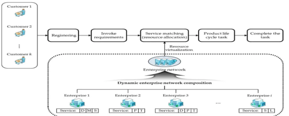
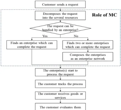
In this sense, various enterprises participating in CM can share manufacturing resources and cooperate with each other to produce highly-customized manufacturing services even though the services are too large or too complex to handle for one enterprise [5]. In addition, CM can deliver reliable, high-quality, and on-demand manufacturing services for the whole lifecycle of manufacturing, such as design, production, testing, and logistics [6], by enabling the enterprises to freely access every manufacturing service in the manufacturing cloud (MC), without certain expertise in the management of resources used. That is, MC is a main component of cloud manufacturing to utilize the manufacturing process in CM. Thus, we use the terms CM and MC separately to distinguish the manufacturing model (CM) and platform (MC), clarifying the manufacturing process in CM. The MC is a manufacturing platform made up of universal and renewable manufacturing resources with flexibility [7]. In the MC, diversified manufacturing resources can be intelligently sensed and connected into the wider Internet, and automatically managed and controlled by means of the Internet of Things (IoT) and related technologies (e.g., radio frequency identification (RFID), wireless sensor network, embedded system, etc.). Then those are virtualized and encapsulated into the MC, which means they are enrolled in the MC with identification factors (e.g., name, inventory level, location). They can be accessed, invoked, and deployed by means of cloud computing technologies, virtualization technologies, and service-oriented technologies after that. MC automatically analyzes customers’ requests to estimate the required resources and the amount of them to complete the requests. After the estimation, MC finds the appropriate enterprise(s) that could successfully complete the request. If the request is so large that two or more enterprises are needed to complete the request, then MC composes the enterprise network for the request. The formal operation process to complete a customer request in MC is presented in Figure1. As seen in Figure1, if the request is too large for an enterprise to complete it (e.g., the request requires various resources or a lot of resources), MC finds and selects two or more enterprises and composes a network of enterprises [8].
Cloud manufacturing is defined by many researchers: Xu [9] defined CM as “a model for enabling ubiquitous, convenient, on-demand network access to a shared pool of configurable manufacturing resources (e.g., manufacturing software tools, manufacturing equipment, and manufacturing capabilities) that can be rapidly provisioned and released with minimal management effort or service provider interaction”. Meanwhile, Wu et al. [10] defined CM as a “customer-centric manufacturing model that exploits on-demand access to a shared collection of diversified and distributed manufacturing resources to form temporary, reconfigurable production lines which enhance efficiency, reduce product lifecycle costs, and allow for optimal resource loading in response to variable-demand customer generated tasking”.
Figure2illustrates the whole life cycle process of CM [11]: First of all, enterprises contract with CM and participate in CM. This contract generates the participation contract cost. Once the enterprise takes part in CM, it is possible to collect the resource information of each enterprise, such as the amount of resources the enterprise currently reserves, which is virtualized and encapsulated in the MC. Customers participating in CM invoke requirements about the products or services they want and the requirements are reorganized to be recognized as demands in CM. Types of resources, due dates, the amount of resources, and so forth, are included in the requests. After that, customer demands are matched with the adequate manufacturing service in the MC considering the information about the resource capabilities of each enterprise. The type of matching requirements and services could be either one-to-one (one enterprise is assigned to the service of one customer), N-to-one (two or more enterprises are assigned to the service of one customer), one-to-N (one enterprise is assigned to the service of two or more customers), or N-to-N (two or more enterprises are assigned to the service of two or more customers). N enterprises compose a temporary production network for one-to-N and N-to-N cases, while there is no need to compose the network for one-to-one and N-to-one cases. Finally, some enterprises in CM may leave CM, which generates a contract cancellation cost.
Figure 2.The whole life cycle process of CM.
shown in Figure1. For convenience, let the amount of every resource be 1. Then, the enterprise alliance that can handle the request from the customer 1 is one of {(enterprise 1, enterprise 2, enterprise 3), (enterprise 1, enterprise 2), (enterprise 1, enterprise 3), (enterprise 3), . . . }. For instance, (enterprise 1, enterprise 2) can handle the demand by sharing D (by enterprise 1), P, and T (by enterprise 2). This indicates that the request can be handled by two or more enterprises (N-to-one) or only one enterprise (one-to-one). Note that enterprise n is not included in any alliance because it does not have either D, P, or T. After an alliance (i.e., temporary production network) is decided to handle the request and the request is fully processed, the alliance is terminated.
Due to the appearance of CM, it is possible for SMEs to perform large-scale and highly customized production by collaborating with other SMEs, but there still remain issues to be solved for practical operation in many aspects. Service selection, scheduling, resource allocation, and capacity-sharing are such issues and, therefore, researchers have recently focused on resolving these issues. For example, Laili et al. [12] analyzed the complex features of cloud services in cloud computing, and based on these features, they suggested a ranking chaos algorithm for service composition selection, and optimal computing resource allocation altogether in the private cloud. In Cao et al. [13], the authors adopted a fuzzy decision-making theory to establish a manufacturing scheduling model in the MC considering four criteria: time, quality, cost, and service. Mai et al. [14] proposed a framework for 3D printing services in the MC to handle several problems of the MC, such as evaluation, service matching, scheduling, etc. Li et al. [15] developed a model to solve industrial robot task allocation problems in CM. This model has three sub strategies, which are the load-balance of robots, minimizing cost, and minimizing processing time, where a genetic algorithm (GA) implements these strategies. Wei et al. [16] adopted an ant colony optimization algorithm for resource allocation problems in CM, where time, cost, quality, and load balance are considered as a multi-dimensional objective function. Tsai et al. [17] employed an improved differential evolution algorithm to optimize task scheduling and resource allocation in a cloud computing environment. Ren et al. [18] analyzed the impact of cooperative relationships between service providers on CM performances, such as the manufacturing task competition rate, service utilization, and service scheduling deviation degree. They showed that the cooperation among enterprises which participate in CM can utilize wasted manufacturing resources, such as idle machines. Argoneto and Renna [19] proposed a framework for capacity-sharing among independent enterprises in CM. The framework, based on a cooperative game algorithm and a fuzzy engine, yields a stable matching among enterprises considering their capacity and geographical locations. Renna [20] developed a decision model for a SME to decide whether to participate or leave a collaborative network, which could be practically applied to CM environments.
As introduced above, research regarding service selection, scheduling, resource allocation, and capacity sharing in CM has been conducted, but there is no previous research considering the dynamic aspects of operation process in CM. In other words, resource allocation or scheduling should be dynamically changed according to dynamically changing customer requests.
Unfortunately, dynamic aspects of the issues in CM have not been fully addressed by the previous researches. For example, the models developed in Cao et al. [13] and Wei et al. [16] yields a manufacturing schedule, and the model developed in Li et al. [15] allocates tasks only before the manufacturing process begins. In other words, their models cannot be applied to real-time situations. As another example, Ren et al. [18] showed the fact that the cooperative relationship between service providers can utilize wasted manufacturing resources, but do not consider the fact that the relationships among manufacturing service providers are changeable in CM.
proposed framework is superior to other frameworks. Ma et al. [23] developed a dynamic task scheduling algorithm based on GA to effectively solve the task scheduling problems in cloud computing environments. Their simulation showed that the proposed algorithm significantly reduced the execution time of task scheduling. Sethanan et al. [24] solved reentrant flow shop scheduling with time windows using hybrid GA, which yields the best solution among meta-heuristic algorithms (simulated annealing, GA, and hybrid GA).
Enterprises which participate in CM should be considered as an inventory unit for scheduling or resource allocation since their resources ensure the circulation of whole manufacturing activities by cooperating with each other in the production network. It is very important, therefore, to compose an enterprise network that handles the requirements from customers (i.e., demands) with minimal costs, and this problem is called the enterprise network composition problem in CM. It is a non-trivial problem since trade-offs exist between costs (e.g. contract cost and opportunity cost of production), and also probabilistic constraints such as forecasted demand and, therefore, it is almost impossible to find the optimal network analytically. This paper proposes a dynamic enterprise network composition algorithm (DENCA) based on a GA to solve the problem dynamically. In other words, DENCA constructs the initial enterprise network and changes the network as demand is changed.
The rest of this paper is organized as follows: Section2describes a research problem called the enterprise network composition problem and introduces assumptions and notations used throughout this paper; Section3proposes an algorithm to solve the problem, and each step of the algorithm is explained in detail; Section4provides a numerical simulation to illustrate the suggested algorithm; and Section5concludes the paper.
2. Enterprise Network Composition Problem
2.1. Description
Since one of the typical characteristics of CM is the pay-per-use of manufacturing resources on demand [5], the cost structures of existing manufacturing models and those of CM are completely different. For example, the task of inventory management for existing manufacturing models is to maintain stock of products or resources [25], while the task for CM is to sustain an appropriate enterprise network to handle various customer requests and minimize the composition cost. Note that the CM task mentioned above is the responsibility of a CM manager, not a manager of an enterprise belonging to CM. Therefore, traditional inventory costs, such as order cost and depreciation cost, are not involved, but enterprise management costs, such as contracts, service invocation, and aggregation, occur in CM [26].
resources an enterprise network has (currently retains). The enterprise management cost, including resource virtualization cost, is the typical example.
It can be intuitively known that there are trade-offs among the costs. For example, if CM contracts many enterprises to participate in CM, then the opportunity cost of production may decrease, while the enterprise management cost will increase. Another example is a trade-off between the participation contract (or contract cancellation) cost and the opportunity cost of production. If a CM manager decides to frequently change the network according to forecasted demands for a flexible operation, then the opportunity cost of production would be minimized, but contract costs and contract cancellation costs would increase. Hence, it is essential to consider these trade-offs for composing a network of enterprises. We call this the enterprise network composition problem throughout the paper.
In Figure3, a dotted rectangle indicates the scope of the paper. We develop an algorithm to compose the enterprise network, which helps CM to match services by ensuring proper levels of demand response. It does not include resource allocation, service matching, and scheduling.
E = , , ⋯ ,
=
PE
Figure 3.Operation process of cloud manufacturing.
2.2. Assumptions and Notations
Initial demand (i.e., demand on day 1) is assumed to be given in advance, while subsequent demands after day 1 must be forecasted. The demands for any manufacturing services are decomposed of each type of required resource. For instance, a demand may be composed of one design resource, two production resources, and one logistics resource. The resources a network retains, but not uses, are always available whenever relevant requests arrive at the MC. If there are not sufficient resources for completing the requests, then the requests will be lost. In addition, contracts regarding enterprise participation in, or withdrawal from, the MC will take effect after a day. In other words, if a company contracts a MC to participate in, or cancel, the contracts to leave the system, then the company will join or leave the system on the next day. Finally, some events to make resources unavailable, such as unexpected maintenance, are not introduced in this paper, but we can introduce the unexpected maintenance into the model by letting the available resources be zeroes during the maintenance period.
Notations used throughout the paper are presented in the following Table1.
Table 1.Notations.
Notation Definition
Ei Enterprisei,i=1, 2,· · ·,n
Iit Indicator variable which represents whether the enterprisethat is,I ijoins the network at daytor not, it=0 or 1
Table 1.Cont.
Notation Definition
Dt
j Demand of Rjat dayt
Dt Vector of demands at dayt, D1t, D2t, · · ·,Dmt
ˆ Dt
j Forecasted demand of Rjat dayt λj(Ei) Ei’s capacity of resource Rj
λj PEt
Current enterprise network’s capacity of resource Rj CIN PEt
Internal management cost of MC ofPEt
CSI(Ei) Cloud service invocation cost of Ei CSA(Ei) Cloud service aggregation cost of Ei CCO(Ei) Participation contract cost of Ei CCW(Ei) Contract cancellation cost of Ei CLO PEt
Opportunity cost of production occurring whenPEtdo not respond demand properly at dayt CSI,Rj Unit cost of cloud service invocation for Rj
CSA,Rj Unit cost of cloud service aggregation for Rj CCO,Rj Unit cost of participation contract for Rj CCW,Rj Unit cost of contract cancellation for Rj CLO,Rj Unit opportunity cost of production for Rj
α Significance level of the risk that demand is unmet (user-defined parameter) τ Number of operation days of MC (user-defined parameter)
3. Dynamic Enterprise Network Composition Algorithm
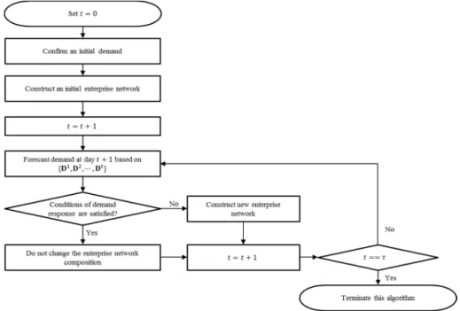
Figure4is a flow chart of the dynamic enterprise network composition algorithm (DENCA) suggested in this research. Initially, the operation day (indicated byt) is set to 0 and initial demand D1is given. Then the CM manager constructs an initial enterprise network that can fully respond to the initial demand with minimal cost. With the networkPEtat daytwhich handles the current demand, the manager forecasts demand at day (t+1) based onD1,D2, . . . ,Dtand decides whether the current networkPEtcan handle the predicted demand ˆDt+1or not. In addition, it should take into consideration that a large portion of resources retained in the current MC may not be used and wasted (i.e., utilization of MC is low) because many unnecessary enterprises are participating in the present MC. Unless the current network is expected to be satisfied with the conditions (the enterprise network is able to handle future demand properly, and resource waste problems should not occur), the manager should construct a new enterprise network and these steps repeat for the entire operating time span.
R = , ⋯ ,
R
, , ⋯ , R
E E R
R C
E E
E E
E E
E E
, R
, R
, R
, R
, R
+
A detailed explanation of the flowchart in Figure4 will be provided from Sections 3.1–3.4. More concretely, Sections3.1and3.2describe how to construct an initial enterprise network and to forecast demand at dayt+1 based on
D1,D2, . . . , Dt , respectively. In Section3.3, we explain how one can check if constraints of the demand response are satisfied and, finally, Section3.4explains the way to construct a new enterprise network when the conditions of the demand response are not satisfied utilizing a genetic algorithm.
3.1. Initial Enterprise Network Composition
The initial enterprise network should cover the initial demands with minimal cost. The formulation for the initial enterprise network composition problem is presented in Equations (1) and (2). The objective function in Equation (1) is to minimize the cost when the initial network is PE1, which consists of the CM internal management cost (CIN(PE1)) and the participation contract cost (∑ni=1 I1
i ×Cco(Ei)
). Note that the contract cancellation and opportunity cost of production are not included in the objective function in Equation (1) because the initial network is constructed to handle the initial demand without any loss. Constraints in Equation (2) imply that the number of resources Rj (j=1, 2,· · ·,m)the initial network possesses must be larger than, or equal to, the initial demand of Rj.
MinZ=CINPE1+ n
∑
i=1
Ii1 ×Cco(Ei)
(1)
subject to:
∑
ni=1Ii1×λj(Ei)≥D1j, for allj=1, 2, . . . , m, Ii1∈ {0, 1} (2) The internal management cost of the MC in Equation (1) is calculated as follows:CIN PEt
=
∑
Ej∈PEt
CSI Ej
+CSA Ej (3)
Cloud service invocation, cloud service aggregation, and participation contraction costs of Eiare calculated in Equations (4)–(6), respectively:
CSI(Ei) = m
∑
j=1
λj(Ei)× CSI, R j
(4)
CSA(Ei) = m
∑
j=1
λj(Ei)× CSA, R j
(5)
CCO(Ei) = m
∑
j=1
λj(Ei)× CCO,R j
(6)
where CSI, Rj, CSA, Rj, and CCO,Rj denote the unit cost of cloud service invocation, cloud service aggregation, and participation contraction for Rj. CSI,Rj is interpreted as the cost to aggregate one additional resource Rj.CSA, Rj andCCO,Rj can be interpreted similarly. Equations (4)–(6) indicate that these costs are directly proportional to the amount and kind of resource Eihas. Thus, the objective function in Equation (1) can be re-written as follows:
MinZ= ∑ Ej∈PE1
( m ∑ j=1
λj(Ei)× CSA, R j
+ ∑m
j=1
λj(Ei)× CSI, R j
)
+ ∑n
i=1 I1
i × m ∑ j=1
λj(Ei)× CCO, R j
!
(7)
The initial enterprise network composition problem can be solved by integer linear programming (ILP), whose decision variableI1
3.2. Resource Demand Forecasting
Time-series analysis methods have been employed to forecast demand of enterprise resources, including cloud computing resources, in many studies. For example, Zhang et al. [28] employed auto-regressive (AR) functions to forecast demand for CPU and memory in a cloud computing environment. LetT(·)be a time-series model for forecasting demandDjt+1 (j=1, 2, . . . , m) at t+1. Then:
Dtj+1=TD1j, · · ·, Dtj+εj =Dˆt+1
j +εj (8)
where the forecasting errorεjis assumed to follow a Gaussian distribution with mean 0 and variance σj2, which is time-independent. Therefore,Dt+1
j is a random variable which also follows a Gaussian distribution with mean ˆDtj+1and varianceσj2. Then we have:
Dt+1= (T(D1), · · ·, T(Dm))T+ε (9)
whereT Dj=TD1
j, · · ·, Dtj
forj=1, 2,· · ·, mandε= (ε1, ε2, · · ·, εm)T.
Note that theDtj denotes the amount of resourcejrequired at dayt. For instance, if a task which requires three resourcejfor two days is arrived at dayt, and there is no other task in CM but the task, then theDtjandDtj+1will be 3.
3.3. Conditions of Demand Response
The condition in Equation (10) helps us determine whether the current network should be reconstructed or not in order to handle the current demands properly and not to waste resources:
P
∑
ni=1 Iit×λj(Ei)<Dˆtj+1
<αforj=1, 2, . . . , m (10)
Inequality in Equation (10) indicates the probability that the capacity of Rj (j=1, 2,· · ·,m)in the current enterprise network is not sufficient for the demand of the next day and should be smaller than user parameterα, the threshold of the risk that demand will not be met. Notice that the value ofα should be small if the loss unit cost is high. By means of a standard normal distribution, the probability can easily be calculated. Another set of inequalities to be considered is the following:
P
∑
Ei∈PEt{PEjt}
Iit×λj(Ei)<Dˆtj+1
<α, forj=1, 2, . . . , m, k=1, 2, . . . , PEt
(11)
Inequality in Equation (11) expresses the probability that an enterprise network could handle the demand properly, even if an arbitrary enterprise currently participating in the MC leaves. This must be larger than 1−α.
3.4. Enterprise Network Recomposition
If the conditions introduced in Section3.3are not satisfied, then the enterprise network should be newly composed. We call this recomposition of the network. Recomposition is noticeably different from the initial network composition because the demand loss probability must be considered, as well as both contract cancellation cost and opportunity cost of production for the network.
The recomposition procedure can be done by solving the following:
MinZ=∑ni=1Iit+1 ×(CSA(Ei) +CSI(Ei)
+∑E i∈/PEt
Iit+1×CCO(Ei)
+ ∑ Ei∈PEt
1−Iit+1
×CCW(Ei)
+ CLO PEt+1
subject to:
P
∑
ni=1Iit+1×λj(Ei)
<Dˆt+1 j
<α, forj=1, 2, 3, . . . , m. (13)
The first term∑ni=1Iit+1 ×(CSA(Ei) +CSI(Ei)
in Equation (12) denotes total cloud service aggregation and invocation costs incurred by enterprises participating in CM. The second term
∑ Ei∈/PEt
Iit+1×CCO(Ei)
is the total contract cost incurred by newly-participating enterprises.
The third term ∑ Ei∈PEt
1−Iit+1
×CCW(Ei)
is the total contract cancellation cost incurred by
newly-leaving enterprises, whereCCW(Ei)is calculated as following:
CCW(Ei) = m
∑
j=1
λj(Ei)× CCW, R j
(14)
Finally,CLO PEt+1
denotes the opportunity cost of production when the enterprise network is PEt+1, which is given by:
CLO PEt= m
∑
j=1
g
∑
Ei∈PEt
λj(Ei), Djt
×CLO, Rj
(15)
whereg∑E
i∈PEtλj(Ei), Dj
tis the amount of loss for R j.
g
∑
Ei∈PEt
λj(Ei),Djt
=
Djt− ∑ Ei∈PEt
λj(Ei), ifDjt> ∑ Ei∈PEt
λj(Ei),
0, otherwise.
(16)
In contrast to the initial network construction, ILP cannot be adopted to recompose the network because of probabilistic constraints. Instead, a metaheuristic algorithm must be used to solve this efficiently and GA is employed in this paper. We represent the structure of chromosomes as a binary string ofnbits where each bit denotes whether a corresponding enterprise participates in the system or not.
4. Numerical Example
This section provides a numerical example to illustrate and compare efficiencies of the suggested algorithm in this study and the branch-and-bound (B and B) algorithm. In Section4.1, we generate a set of simulated data including information of enterprises and estimated demands for an experiment. In Section4.2, we apply DENCA to this simulated dataset.
4.1. Data
We assume that there are 15 enterprises (E1,· · ·, E15)and five resources (R1,· · ·, R5). The amount of resources each enterprise possesses are presented in Table2. Each resource can be a manufacturing resource (e.g., robot arm, 3D printer), a logistic resource (e.g., truck, airplane), etc. As shown, each enterprise has four or five kinds of resources and, therefore, simple inventory models cannot be applied to this problem.
CM is assumed to operate for 30 days (τ = 30), and the actual and forecasted demands of each resource are shown in Table3((a) and (b)), respectively. Forecasted demands are obtained by adding random noiseεj (j=1,· · ·, 5)to actual demands of each resource for 30 days, where
ε1, ε2, ε3 ∼ N 0, 12
and ε4, ε5 ∼ N 0, 0.52
Table 2.Amount of resources each enterprise reserves.
R1 R2 R3 R4 R5
E1 2 0 1 2 1
E2 4 1 2 0 1
E3 3 1 0 3 2
E4 0 2 1 0 5
E5 5 0 2 1 0
E6 1 1 2 2 0
E7 3 2 1 0 1
E8 0 1 1 3 4
E9 2 1 3 1 0
E10 4 0 1 2 2
E11 1 3 1 0 2
E12 2 1 0 1 1
E13 0 4 1 1 3
E14 3 1 2 0 0
E15 0 5 1 2 1
Table 3.The amount of resources each enterprise reserves.
(a) Actual Demands (b) Forecasted Demands
t D1t D2t D3t D4t D5t Dˆt1 Dˆt2 Dˆ3t Dˆt4 Dˆt5
1 12 7 9 7 10 - - - -
-2 12 7 9 7 10 12 7 8 7 9
3 12 7 9 7 10 13 6 9 7 10
4 12 7 9 5 13 11 6 8 5 13
5 15 9 12 5 13 15 6 12 5 13
6 15 9 12 8 13 16 8 10 7 13
7 15 9 12 8 13 13 8 13 7 12
8 10 8 12 8 12 9 7 12 7 11
9 10 8 12 6 12 8 8 11 5 12
10 10 8 11 6 15 10 8 10 5 15
11 12 7 11 7 15 12 6 11 7 14
12 12 7 11 7 15 11 8 11 6 14
13 12 7 9 7 15 13 6 8 6 15
14 14 8 9 10 15 14 7 8 9 14
15 14 8 9 10 11 15 8 8 9 10
16 14 8 9 10 11 14 8 8 10 11
17 14 9 8 10 11 14 8 8 10 10
18 11 10 8 10 11 9 10 7 10 10
19 11 10 8 8 11 11 9 6 7 10
20 11 10 7 8 7 12 9 6 6 6
21 12 10 7 8 7 10 8 7 8 7
22 12 8 7 8 7 12 8 6 8 7
23 12 8 9 7 7 12 6 8 7 6
24 16 8 9 7 5 16 7 7 6 5
25 16 8 11 6 5 17 7 12 5 4
26 16 7 11 6 9 16 7 11 5 8
27 14 7 11 7 9 14 8 10 8 9
28 14 6 9 7 9 13 5 9 8 8
29 13 5 9 6 10 12 3 11 6 10
30 12 3 6 6 10 12 4 6 6 10
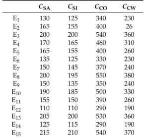
Table 4.Corresponding costs related with each enterprise.
CSA CSI CCO CCW
E1 130 125 340 230
E2 165 155 400 26
E3 200 200 540 360
E4 170 165 460 310
E5 165 155 400 260
E6 135 125 330 230
E7 150 145 370 240
E8 200 195 550 380
E9 150 135 350 240
E10 190 185 500 330
E11 155 150 390 260
E12 110 110 290 190
E13 205 200 530 360
E14 125 115 290 190
E15 215 210 540 370
Table 5.Unit costs of each resource.
R1 R2 R3 R4 R5
CSA,Rk 20 25 20 25 20
CSI,Rk 20 25 15 25 20
CCO,Rk 50 60 40 70 60
CCW,Rk 30 40 30 50 40
CLO,Rk 60 75 60 80 70
4.2. Results
Using the formulation in Section 3.1, we compose the initial network by searching all possible enterprise combinations. In other words, we attempt to find the solution satisfying every constraint and minimizing the costs in Equation (1) from(0, 0, 0, 0, 0, 0, 0, 0, 0, 0, 0, 0, 0, 0, 0) to (1, 1, 1, 1, 1, 1, 1, 1, 1, 1, 1, 1, 1, 1, 1). The optimal initial network, its capacity for each resource, and its related cost are (1, 1, 1, 1, 1, 1, 1, 1, 1, 0, 0, 0, 1, 1, 0), λ1 PE1, . . . , λ5 PE1 = (23, 14, 16, 13, 17), and 18,070, respectively.
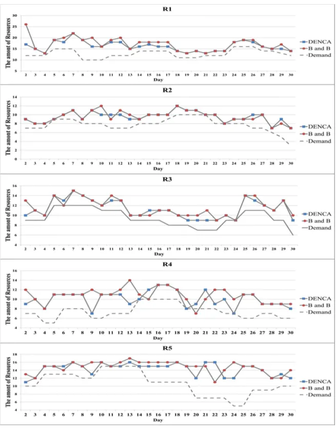
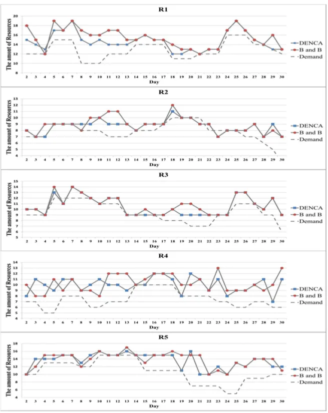
Now, for values α = 0.1 and 0.2, we construct enterprise networks in CM from day 2–30, as explained in Section 3.4, by means of the suggested algorithm, and a B and B algorithm for comparison purpose. The B and B algorithm is employed because it is known to yield good outputs for IP problems in general. Figures5and6illustrate the amount of each resource of the enterprise networks constructed by means of the DENCA and B and B algorithms when α = 0.1 and 0.2, respectively. These figures also include the actual demands for 29 days (from day 2 to day 30).
= .
= .
Figure 6.The amount of each resource the constructed networks own whenα=0.2 and actual demand.
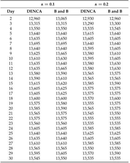
Table 6.Network composition costs by means of the DENCA and B and B algorithms.
α=0.1 α=0.2
Day DENCA B and B DENCA B and B
2 12,960 13,065 12,930 12,960
3 13,315 13,315 13,290 13,300
4 13,550 13,550 13,535 13,545
5 13,640 13,640 13,615 13,640
6 13,635 13,650 13,605 13,605
7 13,695 13,695 13,640 13,640
8 13,640 13,640 13,595 13,605
9 13,625 13,665 13,580 13,610
10 13,610 13,630 13,595 13,605
11 13,635 13,640 13,580 13,630
12 13,635 13,665 13,580 13,630
13 13,580 13,590 13,565 13,575
14 13,590 13,610 13,565 13,565
15 13,615 13,620 13,585 13,590
16 13,605 13,625 13,575 13,575
17 13,605 13,625 13,575 13,575
18 13,600 13,600 13,570 13,600
19 13,575 13,580 13,555 13,575
20 13,585 13,590 13,565 13,575
21 13,565 13,575 13,545 13,550
22 13,575 13,575 13,555 13,555
23 13,560 13,560 13,535 13,535
24 13,605 13,605 13,585 13,585
25 13,640 13,640 13,625 13,625
26 13,635 13,640 13,605 13,605
27 13,610 13,610 13,585 13,585
28 13,565 13,565 13,550 13,550
29 13,595 13,605 13,570 13,590
30 13,545 13,550 13,535 13,535
5. Conclusions
CM can help enterprises (especially SMEs) perform large-scale manufacturing jobs by collaborating with other enterprises, but several critical issues for practical operations remain to be resolved. In this study, we suggested an algorithm based on GA for the enterprise network selection problem, which is one of these problems. This algorithm includes composing an initial enterprise network, forecasting demand, and recomposing the network according to demand forecasts. A numerical example was provided to show that the network constructed by means of the suggested algorithm not only handles the demands better, but also incurs a smaller cost (note that no significant difference was observed between network capacities and actual demands) than the B and B algorithm. In addition, the suggested algorithm is cheaper than the B and B algorithm in terms of computational time.
Since this paper is based on the some assumptions (e.g., the initial demand is given in advance, the forecasting error term follows a Gaussian distribution), this paper may not completely describe and reflect CM situations well. Hence, these assumptions should be eased in our future research. For example, we did not consider the situation that enterprises have trouble in collaborating with each other because of an assumption that enterprises are located near each other. Thus, we will consider collaboration potentials among enterprises based on enterprises’ locations, quality evaluations, etc., in future research.
Author Contributions: Gilseung Ahn, You-Jin Park, and Sun Hur conceived and designed the research; Gilseung Ahn conducted the research and drafted the manuscript. Sun Hur revised the manuscript and You-Jin Park supervised the overall work. All authors read and approved the final manuscript.
Conflicts of Interest:The authors declare no conflict of interest.
References
1. Wang, Z.; Zhang, M.; Sun, H.; Zhu, G. Effects of standardization and innovation on mass customization: An empirical investigation.Technovation2016,48, 79–86. [CrossRef]
2. Ferguson, S.M.; Olewnik, A.T.; Cormier, P. A review of mass customization across marketing, engineering and distribution domains toward development of a process framework. Res. Eng. Des. 2014,25, 11–30. [CrossRef]
3. Li, B.; Zhang, L.; Wang, S.L.; Tao, F.; Cao, J.W.; Jiang, X.D.; Chai, X.D. Cloud manufacturing: A new service-oriented networked manufacturing model.Comput. Integr. Manuf. Syst.2010,16, 1–7.
4. Mell, P.; Grance, T.The NIST Definition of Cloud Computing; National Institute of Standards and Technology: Gaithersburg, MD, USA, 2011.
5. Wu, D.; Greer, M.J.; Rosen, D.W.; Schaefer, D. Cloud manufacturing: drivers, current status, and future trends. In Proceedings of the ASME 2013 International Manufacturing Science and Engineering Conference Collocated with the 41st North American Manufacturing Research Conference, Madison, WI, USA, 10–14 June 2013.
6. Zhang, L.; Luo, Y.; Fan, W.; Tao, F.; Ren, L. Analysis of cloud manufacturing and related advanced manufacturing models.Comput. Integr. Manuf. Syst.2011,17, 458–468.
7. Xu, J.; Chen, P. Study on Objects Ordering for Manufacturing Cloud Platform. In Proceedings of the International Conference on Information Engineering and Applications, London, UK, 26–28 October 2012; pp. 431–437.
8. Huang, B.; Li, C.; Yin, C.; Zhao, X. Cloud manufacturing service platform for small-and medium-sized enterprises.Int. J. Adv. Manuf. Technol.2013,65, 1261–1272. [CrossRef]
9. Xu, X. From cloud computing to cloud manufacturing. Robot. Comput.-Integr. Manuf. 2012, 28, 75–86. [CrossRef]
10. Wu, D.; Rosen, D.W.; Wang, L.; Schaefer, D. Cloud-Based Manufacturing: Old Wine in New Bottles? Procedia CIRP2014,17, 94–99. [CrossRef]
11. Tao, F.; Zhang, L.; Venkatesh, V.C.; Luo, Y.; Cheng, Y. Cloud manufacturing: A computing and service-oriented manufacturing model.J. Eng. Manuf.2011. [CrossRef]
12. Laili, Y.; Tao, F.; Zhang, L.; Cheng, Y.; Luo, Y.; Sarker, B.R. A Ranking Chaos Algorithm for dual scheduling of cloud service and computing resource in private cloud.Comput. Ind.2013,64, 448–463. [CrossRef] 13. Cao, Y.; Wang, S.; Kang, L.; Gao, Y. A TQCS-based service selection and scheduling strategy in cloud
manufacturing.Int. J. Adv. Manuf. Technol.2016,82, 235–251. [CrossRef]
14. Mai, J.; Zhang, L.; Tao, F.; Ren, L. Customized production based on distributed 3D printing services in cloud manufacturing.Int. J. Adv. Manuf. Technol.2016,84, 71–83. [CrossRef]
15. Li, W.; Zhu, C.; Yang, L.T.; Shu, L.; Ngai, E.C.H.; Ma, Y. Subtask Scheduling for Distributed Robots in Cloud Manufacturing.IEEE Syst. J.2015,99, 1–10. [CrossRef]
16. Wei, X.; Liu, H. A cloud manufacturing resource allocation model based on ant colony optimization algorithm. Int. J. Grid Distrib. Comput.2015,8, 55–66. [CrossRef]
17. Tsai, J.T.; Fang, J.C.; Chou, J.H. Optimized task scheduling and resource allocation on cloud computing environment using improved differential evolution algorithm. Comput. Oper. Res. 2013,40, 3045–3055. [CrossRef]
18. Ren, L.; Cui, J.; Wei, Y.; LaiLi, Y.; Zhang, L. Research on the impact of service provider cooperative relationship on cloud manufacturing platform.Int. J. Adv. Manuf. Technol.2016,86, 2279–2290. [CrossRef]
19. Argoneto, P.; Renna, P. Supporting capacity sharing in the cloud manufacturing environment based on game theory and fuzzy logic.Enterp. Inf. Syst.2016,10, 193–210. [CrossRef]
21. Rahman, H.F.; Sarker, R.; Essam, D. A real-time order acceptance and scheduling approach for permutation flow shop problems.Eur. J. Oper. Res.2015,247, 488–503. [CrossRef]
22. Lei, H.; Wang, R.; Zhang, T.; Liu, Y.; Zha, Y. A multi-objective co-evolutionary algorithm for energy-efficient scheduling on a green data center.Comput. Oper. Res.2016,75, 103–117. [CrossRef]
23. Ma, J.; Li, W.; Fu, T.; Yan, L.; Hu, G. A Novel Dynamic Task Scheduling Algorithm Based on Improved Genetic Algorithm in Cloud Computing. InWireless Communications, Networking and Applications; Springer: New Delhi, Germany, 2016; pp. 829–835.
24. Sethanan, K.; Chamnanlor, C.; Chien, C.; Gen, M. Hybrid Genetic Algorithms for Solving Reentrant Flow-Shop Scheduling with Time Windows.Ind. Eng. Manag. Syst.2013,12, 306–316.
25. Basu, R.; Wright, J. Inventory management. InTotal Supply Chain Management; Routledge: London, UK, 2010; pp. 96–108.
26. Chen, F.; Dou, R.; Li, M.; Wu, H. A flexible QoS-aware Web service composition method by multi-objective optimization in cloud manufacturing.Comput. Ind. Eng.2016,99, 423–431. [CrossRef]
27. Cheng, Y.; Zhao, D.; Hu, A.R.; Luo, Y.L.; Tao, F.; Zhang, L. Multi-view models for cost constitution of cloud service in cloud manufacturing system. InAdvances in Computer Science and Education Applications, Proceedings of the International Conference, CSE 2011, Qingdao, China, 9–10 July 2011; Springer: Berlin/Heidelberg, Germany, 2011; pp. 225–233.
28. Zhang, Q.; Zhani, M.F.; Zhang, S.; Zhu, Q.; Boutaba, R.; Hellerstein, J.L. Dynamic energy-aware capacity provisioning for cloud computing environments. In Proceedings of the 9th international conference on Autonomic computing, San Jose, CA, USA, 16–20 September 2012; pp. 145–154.
![Figure 2 illustrates the whole life cycle process of CM [ 11 ]: First of all, enterprises contract with CM and participate in CM](https://thumb-ap.123doks.com/thumbv2/123deta/6882358.248239/3.892.159.735.642.1043/figure-illustrates-life-cycle-process-enterprises-contract-participate.webp)