A uthor(s )
F ujishige, S atoru; S ano, Y oshio; Z han, Ping
C itation
A C M T ransactions on E conomics and C omputation (2018),
6(1)
Is s ue D ate
2018-01-22
UR L
http://hdl.handle.net/2433/228999
R ig ht
©
A C M, 2018. T his is the author's version of the work. It is
posted here by permission of A C M for your personal use. Not
for redistribution. T he definitive version was published in
PUB L IC A T ION, [V olume 6 Issue 1, J anuary 2018, A rticle No.
3] http://doi.acm.org/10.1145/3175496; T his is not the
published version. Please cite only the published version. この
論文は出版社版でありません。引用の際には出版社版を
ご確認ご利用ください。
T ype
J ournal A rticle
The Random Assignment Problem with Submodular Constraints on
Goods
SATORU FUJISHIGE
∗,
Kyoto University, JapanYOSHIO SANO,
University of Tsukuba, JapanPING ZHAN,
Edogawa University, JapanProblems of allocating indivisible goods to agents in an eicient and fair manner without money have long been investigated in the literature. The random assignment problem is one of them, where we are given a ixed feasible (available) set of indivisible goods and a proile of ordinal preferences over the goods, one for each agent. Then, using lotteries, we determine an assignment of goods to agents in a randomized way. A seminal paper of Bogomolnaia and Moulin (2001) shows a probabilistic serial (PS) mechanism to give an ordinally eicient and envy-free solution to the assignment problem.
In this paper we consider an extension of the random assignment problem to submodular constraints on goods. We show that the approach of the PS mechanism by Bogomolnaia and Moulin is powerful enough to solve the random assignment problem with submodular (matroidal and polymatroidal) constraints. Under the agents’ ordinal preferences over goods we show the following.
(1) The obtained PS solution for the problem with unit demands and matroidal constraints is ordinally eicient, envy-free, and weakly strategy-proof with respect to the associated stochastic dominance relation.
(2) For the multi-unit demand and polymatroidal constraint problem the PS solution is ordinally eicient and envy-free but is not strategy-proof in general. However, we show that under a mild condition (that is likely to be satisied in practice) the PS solution is a weak Nash equilibrium.
CCS Concepts: ·Theory of computation→Algorithmic game theory and mechanism design;Discrete optimization;
Additional Key Words and Phrases: Random assignment, probabilistic serial mechanism, ordinal preference, matchings, polymatroids, independent lows, submodular optimization, weak Nash equilibrium
ACM Reference Format:
Satoru FUJISHIGE, Yoshio SANO, and Ping ZHAN. 2017. The Random Assignment Problem with Submodular Constraints on Goods. 1, 1, Article 1 (October 2017), 27 pages.
https://doi.org/10.1145/nnnnnnn.nnnnnnn
1
INTRODUCTION
Problems of allocating indivisible goods to agents in a fair and eicient manner without money have long been investigated in the literature (see, e.g., [1ś6, 17ś22, 26, 28, 31]). Suppose that we are given a ixed feasible (available) set of indivisible goods and a proile of ordinal preferences over the goods, one for each agent. Then, using lotteries, we determine an assignment of goods to agents in a randomized way. A seminal paper of Bogomolnaia
∗The corresponding author
S. Fujishige’s work is supported by JSPS KAKENHI Grant Number JP25280004 and Y. Sano’s work by JSPS KAKENHI Grant Numbers JP15K20885, JP16H03118.
ACM acknowledges that this contribution was authored or co-authored by an employee, contractor, or ailiate of the United States government. As such, the United States government retains a nonexclusive, royalty-free right to publish or reproduce this article, or to allow others to do so, for government purposes only.
© 2017 Association for Computing Machinery. XXXX-XXXX/2017/10-ART1 $15.00
and Moulin [5] shows a probabilistic serial (PS) mechanism to give an ordinally eicient and envy-free solution to the assignment problem.
In this paper we consider an extension of the random assignment problem to submodular constraints on goods in two cases:
(1) Agents have unit demands and the family of feasible sets of goods forms a family of bases of a matroid. (The original problem in [5] is concerned with a matroid having only one base.)
(2) Agents have multi-unit demands and the set of feasible integral vectors of goods forms an integral polyma-troid. (A polymatroid having only one base is treated in [6, 18, 21].)
We show that the approach of the PS mechanism by Bogomolnaia and Moulin [5] is powerful enough to solve the random assignment problem with submodular (matroidal and polymatroidal) constraints. Under the agents’ ordinal preferences over goods we prove the following.
(1) The obtained PS solution for the problem with unit demands and matroidal constraints is ordinally eicient, envy-free, and weakly strategy-proof with respect to the partial order deined by the stochastic dominance relation introduced by Bogomolnaia and Moulin [5].
(2) For the multi-unit demand and polymatroidal constraint problem the PS solution is ordinally eicient and envy-free but is not weakly strategy-proof in general. However, under a mild condition (that is likely to be satisied in practice) the PS solution is a weak Nash equilibrium.
The well-known Birkhof-von Neumann theorem on bi-stochastic matrices shows that every bi-stochastic matrix is expressed as a convex combination of permutation matrices, which plays a crucial role in implementing the PS mechanism developed by Bogomolnaia and Moulin [5]. On the other hand, our extended probabilistic serial mechanism heavily depends on the results of submodular optimization such as the integrality of the independent low polyhedra ([8, 10]), which generalizes the Birkhof-von Neumann theorem.
The present paper is organized as follows. In Section 2 we explain how we are motivated by the seminal paper of Bogomolnaia and Moulin [5]. Section 3 gives some deinitions and preliminaries to be used later. In Section 4 we precisely describe the random assignment problem with submodular (polymatroidal and matroidal) constraints. In Section 5 we show a procedure to ind an extended PS solution in the convex hull of the feasible allocations (as an expected allocation) in an ordinally eicient and fair manner. In Section 6 we examine the issue of strategy-proofness of our solution mechanism. Section 7 shows how to design a lottery eiciently to get the desired expected allocation given in Section 5. Section 8 gives concluding remarks.
The present paper is based on the authors’ working papers [12] and [13].
2
MOTIVATION AND EXAMPLES
In this section we explain our motivation of the present paper through a series of examples of the random assignment problem and their extensions, which hopefully makes our paper more readable for those who are not very familiar with matroids and polymatroids. (Precise deinitions of matroid and polymatroid will be given in Section 3.)
We are interested in obtaining a general model of the random assignment problem, fully generalized in view of the state of the art in combinatorial optimization, to which the PS mechanism of Bogomolnaia and Moulin can naturally be extended. In the history of the developments in combinatorial optimization we have a sequence of successful generalizations of the theory of combinatorial optimization as follows (see, e.g., [10, 27]).
(1) Matchings in bipartite graphs (from around 1930s). (2) From (1) to lows in capacitated networks (from 1950s).
(3) From (1) to matroid intersection (the intersection of two matroids) (from late 1960s).
(We should also mention other successful developments in the theory of combinatorial optimization such as matchings in general graphs and arborescences/branchings in directed graphs, which are not related to the motivation of our present paper.) Another important theoretical development that motivated our present research is the theory of principal partitions [9, 11], which is closely related to convex optimization over polymatroid base polyhedra.
When we found the seminal paper of Bogomolnaia and Moulin [5], we thought that the theory was at the stage of (1) matchings in bipartite graphs and that the probabilistic serial (PS) mechanism shown in [5] was closely related to the monotone algorithm in [9] and [10, Sec. 9.2]. Hence we felt that the results in [5] could naturally be extended to the combinatorial optimization model of (4) mentioned above. Actually, we have found that the PS mechanism of Bogomolnaia and Moulin [5] is powerful enough to have natural extensions to the combinatorial optimization model (4) of independent lows. The full extension of the PS mechanism of Bogomolnaia and Moulin [5] is worth investigating theoretically and it must also be useful for possible applications in the future if not at present.
We hope that readers would duly recognize the potential applicability of our theoretical extensions in practice through (rather toy) examples given below. The issues of ordinal eiciency, envy-freeness, and weak strategy-proofness will be examined later. (LetRbe the set of reals,Zthe set of integers,R≥0the set of nonnegative reals,Z≥0the set of nonnegative integers,R>0the set of positive reals, andZ>0the set of positive integers.) In the following we give six illustrative examples, where the last two examples, Examples 2.5 and 2.6, cannot be modeled by using known PS extensions in the literature.
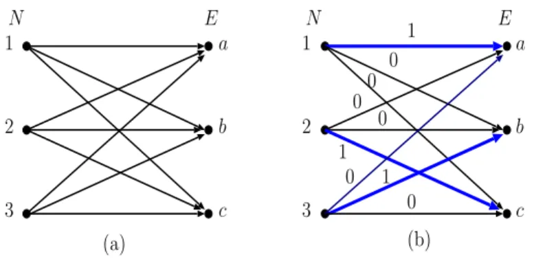
Example 2.1. LetN ={1,2,3}be the set of three agents and suppose that there is only one good (object)e0.
Each agent wants to get the good. This can be illustrated by a graph as in Figure 1 (a). Each feasible assignment
1
3
2 e0
N
1
3
2 e0
1
0
0
(a) (b)
Fig. 1. (a) A simple assignment problem represented by a graph and (b) a feasible{0,1}-flow.
can be identiied with a{0,1}-valued lowφfromN toe0of low value 1 in the graph as in Figure 1 (b). Putting
the set of arcs of the graph asA={(1,e0),(2,e0),(3,e0)}, the set of feasible assignments is represented by the set
of{0,1}-valued vectors in{0,1}A⊂RAasB ={(1,0,0),(0,1,0),(0,0,1)}. Introducing a lottery with a probability distributionponB, we get an expected allocation(p1,p2,p3)with probabilityp1for(1,0,0),p2for(0,1,0), and
p3for(0,0,1). The set of all expected allocations for all possible probability distributionsponBis the convex hull ofB(see Figure 2). Here we do not discuss which expected solution to choose although it is well-known that the solution(13,13,13)obtained by the uniform distribution onBis the fair and strategy-proof solution.
Example 2.2. LetN ={1,2,3}and suppose that we have a setE={a,b,c}of three goods. Each agenti ∈N wants to get one ofEand has a preference order onE. Then any feasible allocation is a perfect matching in the bipartite graphG = (N,E;A)given as in Figure 3 (a). A perfect matching inGcan be identiied with a
O
(1,0,0)
(0,1,0) (0,0,1)
x(1)
x(3)
x(2)
Fig. 2. The set of all expected allocations for Example 2.1.
everye∈E. LetMbe the set of all feasible allocations, i.e., the set of all perfect matchings ofG. We regard every perfect matching inGas a{0,1}-vector inRA. Then every lottery onMdetermines an expected allocation that is a vector in the convex hull Conv(M)ofMinRA. Note that all the possible lotteries onMgenerate exactly the points of the convex hull Conv(M)inRA, which is known as the Birkhof-von Neumann polytope of bi-stochastic matrices. Now the problem is how to determine a solution, a desired expected allocation in Conv(M)and to design a lottery that realizes the solution. This is exactly the model treated by Bogomolnaia and Moulin [5].
1
2
3
a
b
c
1
2
3
a
b
c
(a) (b)
1 0 0 0
0 1
0 1
0
N E N E
Fig. 3. (a) A bipartite graphG=(N,E;A)and (b) a perfect matching as a feasible flow inGfor Example 2.2.
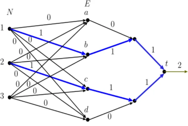
Example 2.3. LetN ={1,2,3}. Now suppose that we have a setE={a,b,c,d}of four goods and that because of some budget constraint only two goods fromEcan be ofered to the agents, while each agent wants to get one good fromEand has a preference order onE. Every feasible allocation for the present problem can be regarded as a{0,1}-valued lowφof low value two fromN toEin the bipartite graphG=(N,E;A)(given as in Figure 4) such that a low of value 0 or 1 enters everyi∈N and a low of value 0 or 1 leaves everye ∈E. Figure 4 shows a feasible allocation that assigns goodcto agent 1 and gooddto agent 2.
1
2
3
a
b
c
d
0
1 0 0
1 0
0 0
0 0 0
0
N E
Fig. 4. A feasible flow in a bipartite graphG=(N,E;A)for Example 2.3.
constraint can be treated as a network low model as in Figure 5, where every feasible allocation can be regarded as a{0,1}-valued lowφ in the graph such that a low of value 0 or 1 enters everyi ∈ N,φsatisies the low conservation law at every internal vertexe ∈E, and a low of value two leaves the exitt, where every arc capacity is equal to one.
1
2
3
a
b
c
d
0
1 0 0
1 0
0 0
0 0 0
0
t
0
1 1
0 2
N
E
Fig. 5. (I) A network-flow representation and a feasible flow for Example 2.3.
Example 2.4. Similarly as in Example 2.3 we may also treat, as a matroidal constraint, the case when at most one good from{a,b}, at most one good from{c,d}, and two goods in total are available. This is a matroidal constraint represented by the direct sum of rank-one uniform matroid on{a,b}and that on{c,d}. As can easily be seen, this can also be formulated as a network low model similarly as in Example 2.3 (see Figure 6). Actually these types of constraints here and in Examples 2.3 are considered by E. Budish et al. [6] as a laminar constraint1, which can be expressed by a directed tree from the setEof leaves toward the root (exit)t with arcs having appropriate capacities. It should further be noted that beyond the laminar constraints represented by directed
trees as considered by Budish et al. [6], we can consider any directed network fromEto exitt, which represents a (poly)matroidal constraint of network type2.
1
2
3
a
b
c
d
0
1 0 0
1 0
0
0 0 0
0 0
0
1
1
0
1
1
t 2 N
E
Fig. 6. (II) A network-flow representation and a feasible flow for Example 2.4.
Moreover, it should be noted that the convex hull of all the{0,1}-valued lows is given by the set of real-valued lows in the associated network, due to the integrality property of lows in networks with integral capacity functions. This gives a basis for constructing a lottery to realize a desired solution.
Example 2.5. LetN ={1,2,3}andE={a,b,c,d}as in Examples 2.3 and 2.4. Suppose that the setBof available subsets ofEis that of all two-element subsets ofEbut{a,b}, i.e.,
B={X |X ⊂E, |X|=2,X ,{a,b}}. (1) This is a graphic matroid, which can be represented by a graphH =(V,E)withEbeing the edge set as shown in Figure 7. Here the feasible sets inBare exactly the edge subsets that form spanning trees ofH.
c
d
a
b
Fig. 7. A graphH=(V,E)with edge setE={a,b,c,d}.
We can consider any matroidal constraints on the set of available subsets of goods.
Example 2.6. LetN ={1,2,3}andE = {a,b,c,d}. Now we suppose thatEis the set of types of goods and there exist multi-units of each goode∈E. As an example consider a polymatroidal constraint of network type shown in Figure 8. In Figure 8 each arc is given an integer capacity, where+∞is regarded as a suiciently large
1
2
3
a
b
c
d
+∞3
1
2
3
t
3
4
2
7
2
1
1
1
+∞ +∞ +∞ +∞ +∞ +∞ +∞ +∞ +∞ +∞ +∞N
E
Fig. 8. A polymatroidal constraint of network type (an integer atached to each arc denotes the arc capacity).
integer. We suppose that each agenti∈Nhas a demandd(i)(the total number of goods of any types) given by
d(1)=3,d(2)=2,andd(3) =3 and the total amount of available goods (of any types) is equal to 7. Then every feasible allocation corresponds to an integral lowφin the network such that (1) the low value entering each
i ∈Nis at mostd(i), (2) the low value leaving the exittis equal to 7, and (3)φsatisies the capacity constraint of every arc and the low conservation at every internal vertex. An integral feasible lowφis shown in Figure 9. An
1
2
3
a
b
c
d
2
0
1
0
0
0
1
1
1 0
0
1
3
0
1
2
3
3
1
t
7
1
1
1
0
N
E
Fig. 9. An integral flowφin the network (an integer atached to each arc denotes the arc flow value), where agent 1 receives two copies of goodaand one copy of goodc.
the set of vectorsx ∈ZE
≥0deined byx(e) =Pi∈Nφ(i,e) (e∈E)for all feasible integral lowsφin the network. SetBis the set of integral bases of a polymatroid of network type, represented by the subnetwork connecting
E={a,b,c,d}with exitt. Besides such polymatroids of network type we can consider any integral polymatroidal set (an integral base polyhedron) of available good vectors inZE
≥0.
3
DEFINITIONS AND PRELIMINARIES
In this section we give deinitions of some concepts from the theory of matroids and polymatroids and also give preliminary lemmas and theorems to be used in the following (see, e.g., [10, 25, 27, 30]).
LetEbe a nonempty inite set. For any subsetX ⊆Edenote byχX the characteristic vector ofX inRE, i.e.,
χX(e)=1 fore ∈X andχX(e) =0 fore∈E\X. We also write χeinstead ofχ{e}fore∈E. A pair(E,ρ)of setEand a functionρ: 2E →R
≥0is called apolymatroid[7] if the following three conditions
hold (also see [10, 27, 30]). (1) ρ(∅)=0.
(2) For anyX,Y ∈2EwithX ⊆Y we haveρ(X) ≤ρ(Y). (3) For anyX,Y ∈2Ewe haveρ(X)
+ρ(Y) ≥ρ(X ∪Y)+ρ(X ∩Y).3
The functionρis called therank functionof the polymatroid(E,ρ). We assumeρ(E)>0 in the sequel.
For a given polymatroid(E,ρ), let B(ρ)(⊆RE)be thebase polyhedronof the polymatroid (see [10]), which is given by
B(ρ)={x ∈RE | ∀X ⊂E:x(X)≤ρ(X), x(E)=ρ(E)}, (2)
where for anyX ⊆Ewe deinex(X) =Pe∈Xx(e). It should be noted that B(ρ) ⊆RE≥0. Moreover, we have the
following relation between the rank functionρand the base polyhedron B(ρ).
ρ(X)=max{x(X) |x ∈B(ρ)} (∀X ⊆E). (3)
Equations (2) and (3) determine a one-to-one correspondence between the set of rank functionsρ : 2E →Rand the set of base polyhedra B(ρ) ⊂RE. It should be noted that the concept of the base polyhedron of a polymatroid is equivalent to that of thecore of a convex gamedue to Shapley [29].
Also consider the lower hereditary closure of the base polyhedron B(ρ)given by
P(ρ) ={x ∈RE | ∀X ⊆E:x(X) ≤ρ(X)}, (4)
which is called thesubmodular polyhedronassociated with polymatroid(E,ρ). The polytope P(+)(ρ) ≡P(ρ)∩RE≥0
is called theindependence polytopeof polymatroid(E,ρ)and each vector in P(+)(ρ)is called anindependent vector. Note that relation (3) holds when we replace B(ρ)by P(ρ)(respectively, P(+)(ρ)) in (3), as well, and P(ρ)uniquely determines the rank functionρ: 2E →R(see Figure 10).
Given a vectorx ∈P(ρ), a subsetX ofEis calledtightforx(orx-tightfor short) if we havex(X)=ρ(X), and there exists a unique maximalx-tight set, denoted by sat(x), which is equal to the union of all tight sets forx. We also have
sat(x)={e∈E | ∀α >0 :x+α χe <P(ρ)}, (5)
which is the set of elementse ∈Efor which we cannot increasex(e)without leaving P(ρ). Moreover, forx ∈P(ρ) ande∈sat(x)deine
dep(x,e) ={e′∈E| ∃α >0 :x+α(χe−χe′) ∈P(ρ)}. (6)
The following fact is fundamental in the theory of polymatroids and submodular functions.
O
x(1) x(2)
P(ρ)
B(ρ)
x(1)
x(2) x(3)
O
B(ρ)
P(ρ)
Fig. 10. Base polyhedraB(ρ)and submodular polyhedraP(ρ).
Lemma 3.1. Given anyx ∈P(ρ)andX,Y ⊆E, if we havex(X)=ρ(X)andx(Y)=ρ(Y), thenx(X∪Y)=ρ(X∪Y) andx(X ∩Y)=ρ(X∩Y). That is, the set ofx-tight sets is closed with respect to the set union and intersection.
Because of this fact sat(x)forx ∈P(ρ)is the unique maximalx-tight set and dep(x,e)fore ∈sat(x)is the unique minimalx-tight set that includese. (See [10] for more details about these concepts and related facts.)
If the rank functionρof a polymatroid(E,ρ)is integer-valued and satisiesρ({e})≤1 for alle ∈E, then(E,ρ) is called amatroid(see, e.g., [25, 30]). When(E,ρ)is a matroid, deine
I={X ⊆E| |X|=ρ(X)}, B={X ∈ I | |X|=ρ(E)}. (7) EachI ∈ Iis called anindependent setandIis thefamily of independent setsof(E,ρ). EachB∈ Bis called a baseandBis called thefamily of basesand consists of all maximal independent sets of(E,ρ)(maximal with respect to set inclusion). Since each ofρ,BandIuniquely determines the matroid onE, we also denote by (E,B)(or(E,I)) the matroid(E,ρ).
For any polymatroid(E,ρ)with an integer-valued rank functionρdeine
BZ(ρ)=B(ρ)∩ZE, PZ(ρ)=P(ρ)∩ZE. (8)
The following is well known (see, e.g., [10]).
Theorem 3.2. When(E,ρ) is a polymatroid with an integer-valued rank functionρ,B(ρ) (resp.P(ρ))is the convex hull ofBZ(ρ)(resp.PZ(ρ)). Moreover, when(E,ρ)is a matroid,BZ(ρ)(orP(+)(ρ)∩ZE)is exactly the set of
all the characteristic vectors of bases(or independent sets)of matroid(E,ρ).
For a polymatroid(E,ρ)and a nonempty subsetF ⊆EdeineρF : 2F →RbyρF(X)
=ρ(X)for allX ⊆F. Then we have a polymatroid(F,ρF), which is called areduction of (E,ρ) byF (orrestriction of (E,ρ) to F). Moreover, deineρF : 2E\F →RbyρF(X) =ρ(F∪X)−ρ(F)for allX ⊆E\F. Then(E\F,ρF)is a polymatroid, called acontraction of (E,ρ)byF. For any nonemptyF1,F2⊆EwithF1⊂F2we putρF2
F1=(ρ F2)
F1, which deines a polymatroid(F2\F1,ρFF12), called aminorof(E,ρ).
For any vectorx ∈RE and any nonempty setA⊆EdeinexA∈RAbyxA(e)=x(e)for alle ∈A. We have the following lemma, which will be used in Section 6.1.1.
(Proof) Suppose that we are given vectorsx,y∈P(ρ)satisfyingx(e)≥y(e) (∀e ∈E\sat(x)). Increase the values ofy(e)for alle∈sat(x)as much as possible while keeping the vector within P(ρ), and let us denote byy′the resulting vector in P(ρ). Then, we have sat(y′) ⊇sat(x). LettingA
=sat(x)andB=sat(y′), ifρ(A) >y′(A), then
ρ(B)−ρ(A) <y′(B)−y′(A) ≤x(B)−x(A).
Sinceρ(A)=x(A), this impliesρ(B)<x(B), a contradiction. Henceρ(A)=y′(A)and(y′)AandxAare bases of
P·A=(A,ρA), the restriction ofPtoA. Hence(y′)E\A∈P(ρ
A), whereρAis the rank function of the contraction
(E\A,ρA)ofPbyA. Sincex(e) ≥y′(e) (∀e ∈E\A)and sat(x)=A, we have sat(y) ⊆sat(y′) ⊆sat(x)=A. □
Simple examples of polymatroids, some of which has already appeared in Section 2, are given as follows.
Uniform matroids: For a positive integerk ≤m(=|E|)every subset of cardinalityk ofEis exactly a base, i.e.,
B={X |X ⊆E, |X|=k}.
Whenk =m(=|E|),Bconsists of only one baseE, which is the unique available set of goods as considered in the literature for the ordinary random assignment problem.
Graphic matroids: For a connected graphG=(V,E)with a vertex setV and an edge setEevery edge subset
that forms a spanning tree ofGis exactly a base, i.e.,(E,B)is the graphic matroid represented by graphG=(V,E) withBbeing the family of edge sets of spanning trees. Note that for anyX ⊆Ethe value ofρ(X)is equal to the maximum size of cycle-free subsets ofX inG.
Symmetric polymatroids: Letд:R→Rbe a nondecreasing concave function withд(0) =0. Deineρ: 2E →R
byρ(X)=д(|X|). Then(E,ρ)is a polymatroid. Note that the concavity ofдcorresponds to the law of diminishing marginal utility in economics.
Linear polymatroids: LetV be a vector space. LetEbe a nonempty inite set and for eache ∈ EletFebe a
inite set of vectors inV. Deineρ: 2E→Rbyρ(X)
=rank(Se∈XFe)for allX ⊆E. Then(E,ρ)is a polymatroid with the integer-valued rank functionρ.
Polymatroids of multi-terminal network lows([23],[10, Sec 2.2]; also see [9, 15]): LetN =(G=(V,A),s,T,c)
be a network, whereG=(V,A)is a graph with a vertex setV and an arc setA,s ∈V is a source,T ⊂V\ {s}is a set of sink terminals, andc:A→R>0is a capacity function of the network. We suppose that there exists no arc leavingT. A functionφ:A→R≥0is called a feasible low inN if it satisies the capacity constraints
0≤φ(a) ≤c(a) (∀a∈A) (9)
and the low conservation constraints
∂φ(v)=0 (∀v∈V\({s} ∪T)), (10)
where the boundary∂φ:V →Rof lowφis deined by
∂φ(v) = X
(v,w)∈A
φ(v,w)− X
(w,v)∈A
φ(w,v) (∀v∈V). (11)
Also deine the out-low∂−φ :T →R
≥0ofφby
∂−φ(v)= X
(w,v)∈A
φ(w,v) (=−∂φ(v)) (∀v ∈T). (12)
Then the set of out-lows∂−φ ∈ RT
≥0 of all feasible lowsφinN is the independence polytope, inRT≥0, of a
polymatroid(T,ρ)onT. For anyX ⊆T the value of rankρ(X)is equal to the maximum low value fromstoX
When the underlying graphG = (V,A)is a star such thatV ={s} ∪T andA={(s,t) |t ∈T}, we have a polymatroid onT with a modular rank functionρsuch thatρ(X)=Pv∈Xc(s,v)for allX ⊆T. Any polymatroid of this kind has a unique base and vice versa.
Consider a capacitated networkN = (G = (V,A),S+,S−,c,(S+,ρ+),(S−,ρ−)) with polymatroids on sets
S+,S−⊂V. HereGis the underlying graph with vertex setV and arc setA, andS+andS−are disjoint subsets of
V and are, respectively, the set of sources (entrances) and that of sinks (exits). Furthermore, we have a capacity functionc : A → R≥0 and a pair of polymatroids(S+,ρ+) and(S−,ρ−). A functionφ : A → Ris called an independent lowinN if it satisies
0≤φ(a) ≤c(a) (∀a∈A), (13)
∂φ(v)=0 (∀v ∈V \(S+∪S−)), (14) ∂+φ∈P
(+)(ρ+), ∂−φ∈P(+)(ρ−), (15) where∂±φ :S±→Rare deined by∂+φ(v)
=∂φ(v)for allv ∈S+and∂−φ(v) =−∂φ(v)for allv ∈S−. Note that (13) is the low capacity constraint for each arc, (14) the low conservation constraint on each internal vertex, and (15) the polymatroidal boundary constraints on the entrance setS+and the exit setS−. The value ∂+φ(S+)(=∂−φ(S−))is called thelow value(or simplyvalue) of the independent lowφ. We may also consider a cost functionγ :A→R, which gives a problem of inding a minimum-cost independent low inN. This is called theindependent lowproblem [8] and is equivalent to what is called thesubmodular lowproblem (see [10]).
We have the following integrality theorem ([8, 10]), which plays a crucial role in validating our approach based on the PS mechanism of Bogomolnaia and Moulin [5].
Theorem 3.4. LetP∗⊂RAbe the set of all independent lowsφin networkN =(G=(V,A),S+,S−,c,(S+,ρ+),
(S−,ρ−)). Ifcandρ±are integer-valued, thenP∗is an integral polytope, i.e.,P∗is a convex polytope such that every extreme point ofP∗is an integral vector. Moreover, the same integrality property also holds if we consider the set of independent lows of ixed integral value∂+φ(S+)(=∂−φ(S−)).
4
DESCRIPTION OF THE RANDOM ASSIGNMENT PROBLEM
Now we give a precise deinition of the random assignment problem with polymatroidal constraints and later examine the problem with matroidal constraints as a special case.
4.1
Model description
LetN ={1,2,· · ·,n}be a set of agents andEbe a set of goods. Each goode ∈Eshould be considered as a type of good and the number of available goodecan be more than one (see Example 2.6). Each agenti∈Nwants to obtain a certain amount of goods of any types, denoted byd(i) ∈Z>0, at most in total. We refer tod(i)as the demand upper boundof agenti. The vectord =(d(i) |i ∈N)∈ZN>0is called thedemand vector. For eachi∈N
ande∈Eletxi(e)be the number of copies of goodethat agentiobtains. Then we must have
xi(E)≡X
e∈E
xi(e) ≤d(i) (16)
for every agenti ∈N. LetB ⊆ZE
≥0be the set of all available vectors of goods in the market that is given by
B=BZ(ρ)for a polymatroid(E,ρ)with an integer-valued rank functionρ(see (8)). Since the sum of vectors P
i∈Nxi must be available in the market, we have the following constraint.
X
i∈N
xi ∈BZ(ρ). (17)
DeineA⊆ZN×E
≥0 to be the set of all functionsφ:N×E→Z≥0such that vectors given byxi =(φ(i,e) |e∈E) for alli ∈ N satisfy (16) and (17). Everyφ ∈Adetermines a feasible allocationxi
=(φ(i,e) |e ∈E)for each agenti ∈N. Note that a functionφ:N×E→Z≥0is identiied with anN×EmatrixP =(φ(i,e) |i ∈N,e ∈E), andxi is with theith row ofP for eachi ∈N.
Consider an independent-low networkN = (G =(S+,S−;A),c,(S+,ρ+),(S−,ρ−)), whereS+ =N,S− =E,
G=(S+,S−;A)is a complete bipartite graph with vertex bi-partition(S+,S−)and arc setA=S+×S−,c(a)= +∞ (a suiciently large positive integer) for alla∈A,(S−,ρ−)is an integral polymatroid with rank functionρ−=ρ appearing in (17), and(S+,ρ+)is a polymatroid with a (modular) rank functionρ+given byρ+(X)
=d(X)for all
X ⊆S+
=N.4For simplicity we also denote the present independent-low network byN =(N,E,d,(E,ρ))(see Figure 11). Then from Theorem 3.2 we can easily see the following.
Lemma 4.1. The setA is exactly the set of integer-valued independent lowsφ : S+ ×S− → Z
≥0 of value
∂+φ(N)=∂−φ(E)
=ρ(E)in networkN =(N,E,d,(E,ρ)).
P= (E, ρ) E
N
N×E
.. .
.. .
.. .
.. . d(1)
d(n)
∂−ϕ∈P(ρ)
∂+ϕ≤d
Fig. 11. An independent-flow networkN.
Because of Theorem 3.4 and Lemma 4.1 we also have the following.
Corollary 4.2. The set of all(real-valued)independent lowsφ of valueρ(E) inN = (N,E,d,(E,ρ))is the convex hullConv(A)of all integer-valued independent lows of valueρ(E)inN.
4.2
Ordinal preference and stochastic dominance relation
We suppose that each agenti∈N has an ordinalpreference≻iover setEof types of goods5, which is a linear ordering ofE. Let agenti’s preference be given by
Li : e1i ≻i e2i ≻i · · · ≻i eim, (18) 4We may be tempted to consider ageneralpolymatroid as(S+,ρ+)on the setS+=Nof agents instead of a modular rank functionρ+. Though the PS mechanism of Bogomolnaia and Moulin can formally be extended to such a general model mathematically, we cannot adapt our arguments to validate the assertions given in the sequel, especialy in Section 6. However, because of Theorem 3.2 the procedure shown in Section 7 for designing a lottery to realize any given expected allocation can be adapted even for such a general model (cf. the model with a bihierarchy structure in [6]).
where{ei
1,ei2,· · ·,emi }=E6andei1is the most favorite (type of) good for agenti. LetLbe the proile of preferences Li (i ∈N).
Since we must make a decision on how to allocate goods in a fair manner without money, we may consider a lottery, which is represented by a probability distributionpoverA, i.e.,p :A→R≥0satisfyingP
φ∈Ap(φ)=1.
Then theexpectedallocation of goods is given by
E{φ}=X
φ∈A
p(φ)φ, (19)
where precisely speaking, the left-hand side is the expectation of a random variableφ with its probability
distributionponAwhileφappearing on the right-hand side is a variable taking on values ofA. It should be noted that the set of all expected allocationsE{φ}of (19) for all possible probability distributionspis exactly the convex hull Conv(A)ofAand that every lottery picks up a point from among Conv(A).
In the following we useN×EmatricesP to express expected allocationsφ ∈Conv(A)by identifyingφwith
P =(φ(i,e) |i∈N,e ∈E), which is often employed in the literature. So we may writeP ∈Conv(A), for example. Whenφcorresponds toP,φis sometimes written asφP.
An eicient and fair expected allocation will be found with respect to thestochastic dominance relation (sd-dominance relationfor short)⪰isdfor each agenti ∈Non expected allocations deined as follows. Recall that we are given a preference proileL=(Li |i ∈N)of (18). For anyP,Q∈Conv(A), puttingPi =(P(i,e) |e ∈E)and
Qi =(Q(i,e) |e ∈E)for alli ∈N, we deine
Pi ⪰isdQi ⇐⇒ ∀ℓ ∈ {1,· · ·,m}:
ℓ
X
k=1
P(i,eik)≥ ℓ
X
k=1
Q(i,eki). (20)
We say an expected allocationP issd-dominatedbyQif we haveQi ⪰sdi Pi for alli ∈NandP ,Q. We say thatP isordinally eicientifPis not sd-dominated by any other expected allocation in Conv(A)(cf. [5]).
Also, we say an expected allocationP isnormalized envy-free([18]) with respect to preference proileL= (Li |i ∈N)of (18) if we have
1
d(i)Pi ⪰ sd
i 1
d(j)Pj (∀i,j∈N), (21)
whered(i)is the integral demand upper bound of agenti ∈N.
4.3
Lotery
When designing a lottery to pick up a solution (a desired expected allocation), it is crucial to see that we have the integrality property of Conv(A)due to Corollary 4.2. Hence, given any (desired) expected allocationE{φ}in Conv(A), we need at most|N| × |E|(extreme) points inAthat has positive probabilities of occurrence because of Carathéodory’s theorem on convex polytopes in order to realize a lottery that gives the expected allocationE{φ}.
Consequently, our problem becomes the following two:
(1) Find a point ¯φ(= E{φ}) from among the polytope Conv(A) in an ordinally eicient and fair manner according to the preference proileL=(Li |i ∈N).
(2) Construct a lottery by inding a representation of ¯φas a convex combination of integral points of polytope Conv(A). The coeicients of the convex combination provide us with positive probabilities of a probability distribution overAthat leads us to ¯φ=E{φ}in (19).
6We have assumed that the preference is strict and complete, i.e.,m
It heavily depends on the structure of the setAof feasible allocations whether we can ind a desired expected solution ¯φand construct a lottery to realize ¯φin a computationally eicient way. Fortunately, it follows from Theorem 3.4 and Corollary 4.2 thatAis the independent low polytope and has a nice combinatorial structure as shown in the literature (see, e.g., [10]). We will see that the probabilistic serial (PS) mechanism by Bogomolnaia and Moulin [5] works surprisingly well for these general problem settings with submodular constraints.
4.4
Brief historical remarks
The problem considered here includes the following as special cases.
(a) The ordinary random assignment problem considered in the literature is mostly the case whered =1∈ZN>0
andB={1} ⊆ZE
>0(e.g., [4, 5, 20]). Here1denotes a vector of all ones of appropriate dimension (determined
by the context).
(b) Kojima [21], Aziz [2], and Heo [18] considered a multi-unit demand case whered ∈ZN
>0andB={b} ⊆ZE>0
for someb∈ZE
>0.
Note that whenBis a singleton set as in (a) and (b) above, the underlying (poly)matroid(E,ρ)has the unique base and the rank functionρis modular.
5
FINDING AN ORDINALLY EFFICIENT AND FAIR EXPECTED ALLOCATION
We irst show a procedure,Algorithm 1, which is an extension of the PS mechanism of Bogomolnaia and Moulin
[5] and will then show that the computed point in Conv(A)is an ordinally eicient and fair expected allocation. Let us deine the basex∗P ∈B(ρ)associated with an allocationP ∈Conv(A)by
x∗P ≡X
i∈N
Pi. (22)
Recall that for eachi ∈N agenti’s preference is given by (18), where{e1i,ei2,· · ·,eim}=Eandei1is the most favorite (type of) good for agenti, andLis the proile of preferencesLi(i ∈N). Based on the collection (a multiset) of the irst (most favorite) elementsei
1of all agentsi∈N, deine a nonnegative integral vectorb(L)∈ZE≥0by
b(L) =
X
i∈N
d(i)χei
1, (23)
where we may havee1i =e1j for distincti,j∈N andd(i)is the integral demand upper bound of agenti∈N.
We also denote the random assignment problem byRA=(N,E,L=(Li |i∈N),d
=(d(i)|i∈N),(E,ρ)). During the execution of the following algorithm the current preference listsLi may get shorter because of removal of exhausted (or saturated) types of goods. Also note thatSpis the set of types of goods saturated at stagep.
ÐÐÐÐÐÐÐÐÐÐÐÐÐÐÐÐÐÐÐÐÐÐÐÐÐÐÐÐÐÐÐÐÐÐÐÐÐÐÐÐÐÐÐÐÐÐÐÐÐÐÐÐÐÐÐÐÐÐÐÐś
Algorithm 1:Extended PS Solution7
ÐÐÐÐÐÐÐÐÐÐÐÐÐÐÐÐÐÐÐÐÐÐÐÐÐÐÐÐÐÐÐÐÐÐÐÐÐÐÐÐÐÐÐÐÐÐÐÐÐÐÐÐÐÐÐÐÐÐÐÐś
Input: Arandom assignment problemRA=(N,E,L,d,(E,ρ)).
Output: An expected allocationP :N×E→R≥0.
Step 0: For eachi∈N putxi ←0∈RE(the zero vector), andx∗←0∈RE.
PutS0← ∅,p←1, andλ0←0.
Step 1: For current (updated)L =(Li |i ∈N), usingb(L)in (23), compute
λp=max{t≥λp−1 |x∗+(t−λp−1)b(L)∈P(ρ)}. (24)
For eachi ∈N putxi ←xi
+(λp−λp−1)d(i)χei
1. Putx∗←x∗+(λp−λp−1)b(L)andSp←sat(x∗).
Step 2: PutTp←Sp\Sp−1.
UpdateLi (i∈N)by removing all elements ofT
pfrom currentLi (i ∈N).
Step 3: Ifρ(Sp) <ρ(E), then putp←p+1 and go to Step 1.
Otherwise (ρ(Sp)=ρ(E)) putP(i,e) ←xi(e)for alli∈N ande ∈E. ReturnP.
ÐÐÐÐÐÐÐÐÐÐÐÐÐÐÐÐÐÐÐÐÐÐÐÐÐÐÐÐÐÐÐÐÐÐÐÐÐÐÐÐÐÐÐÐÐÐÐÐÐÐÐÐÐÐÐÐÐÐÐÐś
As in [5],the parametertin (24) can be considered as time and each agenti ∈N eats the current top goodei1at rated(i)per unit time.
5.1
Examples
To see the behavior ofAlgorithm 1let us consider two illustrative examples given as follows.
Example I(A graphic matroidal constraint and unit demands): Let us consider a familyBof feasible sets given
by
B={X |X ⊂E, |X|=2,X ,{a,b}}. (25) This is a graphic matroid andBis the family of edge subsets of spanning trees of the graph shown as Figure 7 in Example 2.5.
Suppose that preferences of all agents are given as follows.
i ∈N preference Li
1 a≻1b≻1c≻1d
2 a≻2c≻2b≻2d
3 a≻3c≻3d ≻3b
4 b ≻4a≻4d ≻4c
Also suppose that every agent has a unit demand, i.e.,d =1=(1,1,1,1) ∈ZN. Then byAlgorithm 1we get
P =
*. .. . ,
a b c d
1 1/4 0 1/4 0
2 1/4 0 1/4 0
3 1/4 0 1/4 0
4 0 1/4 0 1/4
+/ // /
-,
where
b(L)=
a b c d
1+1+1, 1, 0, 0, S1={a,b}, λ1=1/4 for p=1 and
b(L)=(0,0,1+1+1,1), S2={a,b,c,d}, λ2=λ1+1/4 for p =2,
and each row sum ofP is equal to 1/4+1/4=1/2. Here, recall thatSpis the set of saturated (or exhausted) goods after thepth execution of Step 1 ofAlgorithm 1. Also, vectorsxλ∗
p onTp =Sp\Sp−1forp=1,2 are given by
T1={a,b}, T2={c,d},
xλ∗
1(a)=3/4, x ∗
λ1(b) =1/4, x ∗
λ2(c)=3/4, x ∗
The following example has a polymatroidal constraint and multi-unit demands and supplies.
Example II: ConsiderN ={1,2,3,4}andE={a,b,c,d}again. Let(E,ρ)be a polymatroid with a rank function
given by
ρ(X) =
(
4|X| if|X| ≤2
8 if|X|>2 (∀X ⊆E). (26)
Note that(E,ρ)here is a symmetric polymatroid. Suppose that preferences of all agents are the same as Example I butE={a,b,c,d}should be regarded as a set of types of goods. Let a demand vector be given byd =(4,2,1,1) ∈
ZN. Then byAlgorithm 1we haveP ∈RN×E
≥0 , as anN×Ematrix, given as follows.
P =
*. .. . ,
a b c d
1 16/7 12/7 0 0
2 8/7 0 6/7 0
3 4/7 0 3/7 0
4 0 4/7+3/7 0 0
+/ // /
-,
where
b(L) =
a b c d
4+2+1, 1, 0, 0, S1={a}, λ1=4/7 for p=1 and
b(L) =(0,4+1,2+1,0), S2={a,b,c,d}, λ2=λ1+3/7 for p=2 to get the expected allocationP given above. Also, vectorsx∗λ
p, which are the restriction ofx
∗
P onTp=Sp\Sp−1 forp=1,2, are given by
T1={a}, T2={b,c,d},
xλ∗1(a)=4, xλ∗2(b)=19/7, x∗λ2(c)=9/7, x∗λ2(d)=0.
HencexP∗ =(4,19/7,9/7,0). Note that∅,{a},{a,b,c}, and{a,b,c,d}(=sat(x∗P))are tight sets forx ∗ P.
5.2
Ordinal eficiency
The following theorem can be shown in a very similar way as the corresponding one in [5]. However, it can be seen that the given proof heavily depends on the underlying submodularity structure, especially the one used for the arguments in [9].
Theorem 5.1. Algorithm 1computes an expected allocation inConv(A)that is ordinally eicient.
(Proof) ByAlgorithm 1we get an expected allocationP in Conv(A)together with a chainS0=∅ ⊂S1⊂ · · · ⊂ Sp=E. LetQbe an arbitrary expected allocation in Conv(A)and suppose thatQ =P orQsd-dominatesP. It suices to proveQ=P.
At theqth execution of Step 1 ofAlgorithm 1deine
Fq={i ∈N |ei1∈Tq}. (27)
Let us denoteei
1(the top element in currentLi) at theqth execution of Step 1 byei1(q)and suppose that for some
integerq∗ ≥1 we have
Q(i,ei1(q))=P(i,ei1(q)) (∀q=1,· · ·,q∗−1, ∀i ∈Fq) (28) and we execute theq∗th Step 1. Then, because of Step 1 ofAlgorithm 1we have
X
i∈Fq
SinceQ=PorQsd-dominatesP, it follows from (28) thatQ(i,ei
1(q∗))≥P(i,e1i(q∗))for alli ∈Fq∗. Hence from (28) and (29) we must have
Q(i,ei1(q∗))=P(i,ei1(q∗)) (∀i∈Fq∗), (30)
since we haveP
i∈Fq∗Q(i,ei1(q∗))≤ρ(Sq∗)−ρ(Sq∗−1). Here note that q∗
X
q=1
X
i∈Fq
Q(i,ei1(q))≤ρ(Sq∗). (31)
Now, note that whenq∗=1, Equation (28) is void (and thus holds). Hence, by induction onq=1,· · ·,p, we have
shownQ=P. □
5.3
Envy-freeness
Recall the deinition of normalized envy-freeness given in Section 4.2. We have the following theorem on normalized envy-freeness of the extended PS mechanism. The proof is actually a direct adaptation of the one given by Bogomolnaia and Moulin [5] and Schulman and Vazirani [28] for existing problem settings (also see [18]). It should be noted that byAlgorithm 1every agenti ∈N eatsd(i)units of goods per unit time, which is equivalent to consideringd(i)copies of every agenti ∈N such that each copy of agentihas the same preference as agentibut has a unit demand.
Theorem 5.2. Algorithm 1computes an expected allocationP that is normalized envy-free.
(Proof) It suices to show that for anyi∈N andk ∈ {1,· · ·,m}we have
1
d(i)
k
X
ℓ=1
P(i,eiℓ) ≥
1
d(j)
k
X
ℓ=1
P(j,eiℓ) (∀j ∈N). (32)
Deine
tki = 1
d(i)
k
X
ℓ=1
P(i,eiℓ). (33)
When goodei
kis removed after an execution of Step 1, all goodse i
ℓ (ℓ=1,· · ·,k)have been removed fromE. It
follows that for allj∈N the time spent by agentjto eateiℓ(ℓ=1,· · ·,k)given by the sum of possible values
1
d(j)P(j,eiℓ)for goodse
i
ℓ (ℓ=1,· · ·,k)is withint
i
k. Hence we must have
tki ≥ 1
d(j)
k
X
ℓ=1
P(j,eiℓ) (∀j∈N). (34)
□
6
STRATEGY-PROOFNESS
It is known that the extension of the PS mechanism of Bogomolnaia and Moulin to the case of multi-unit demands cannot be weakly strategy-proof in general ([3, 6, 18, 21]). Therefore, our polymatroidal extension is not weakly strategy-proof in general either.8
Note that a mechanismMisweakly strategy-proof if foreveryinput preference proileLthe mechanismM
gives a solution (an expected allocation)P such that for each agenti∈Nevery misreport of agenti’s preference
8Schulman and Vazirani [28] showed strategy-proofness of the PS mechanism under lexicographic preferences. It is left for future research to
results in a solutionQsatisfying thatQidoes not sd-dominatePi fori. Here the strategy-proofness is concerned with the mechanism.
6.1
Weak Nash equilibria
Let us consider the concept of aweak Nash equilibrium, which is a property of the obtained solution. For agiven input proilewe say that the solutionPobtained by the mechanismMis aweak Nash equilibriumif for each agent
i ∈Nevery misreport of agenti’s preference results in a solutionQsatisfying thatQi does not sd-dominatePi fori. That is, for a weak Nash equilibriumP no agentican improve her expected allocationPi with respect to the sd-dominance relation by any misreport of her preferenceLi.
We examine our polymatroidal extension and give a certain suicient condition9for our solution to be a weak Nash equilibrium. The result, Theorem 6.3, given below seems to be new even for the ordinary multi-unit demand case where the base polyhedron consists of a single base, i.e., B(ρ)={b}for someb∈ZE
>0. In Section 6.2 we also
prove the weak strategy-proofness in the special case of unit demands and matroidal supplies (shown in [13]).
6.1.1 Lemmas.We irst prepare two lemmas to prove Theorem 6.3 concerned with a condition for our solution to be a weak Nash equilibrium.
Let us consider the ‘eating process’ (due to Bogomolnaia and Moulin [5]). ByAlgorithm 1we havecritical times
λ0=0<λ1 <· · ·<λq=ρ(E)/d(N)
computed by (24), whered(N) =Pi∈Nd(i). At each critical timeλk > 0,L is updated by removing all the saturated types of goods fromL.
For each timetwithλk ≤t≤λk+1fork ∈ {0,· · ·,q−1}we put xt∗=xλ∗k +(t−λk)b(Lt),
whereLt =(Lit |i∈N)denotes the currentL=(Li |i ∈N)at timetand
b(Lt)=
X
i∈N
d(i)χei
1
withei
1being the top element (type of good) of currentLit. We putx0∗=0. Note that we have
sat(xt∗) =sat(x∗λk) (∀t∈[λk,λk+1), ∀k ∈ {0,· · ·,q−1}).
Now, suppose that agent 1∈Nhas a preference listL1and misreports her preference as ¯L1. Put ¯L =(L¯i |i ∈N) with ¯Li
=Lifori∈N\ {1}. For any original objectp(a parameter, a vector, etc.) deined under preference proile
L, let us denote by ¯pthe objectpdeined under misreported preference proile ¯L.
For eache ∈ EdeineNP(e) = {i ∈ N | P(i,e) > 0}. For eache ∈ Elett(e) be the time when goode is exhausted (or saturated). Also for eache∈Eandi∈NP(e)letti0(e)be the time when agentistarts eating goode (or the time whenebecomes the top element of currentLi).
Lemma 6.1. LetL1andL¯1be given by
L1:w1≻ · · · ≻ws ≻a≻ · · ·, (35)
¯
L1:w1≻ · · · ≻ws ≻z1≻ · · · ≻zs′ ≻a≻ · · · (36) withP(1,a)>0for some integerss≥0ands′≥1. Suppose thatt¯(a)>t(a). Then, the following three statements hold during the execution ofAlgorithm 1with current timet<t(a).
(a) For eachi ∈N\ {1}we haveei
1 ⪰i e¯1i, wheree1i ande¯i1are the top elements of currentLitforLt and currentL¯it forL¯t, respectively, and⪰iis the order of originalLi.
(b) For eache ∈E\(sat(x¯∗
t)∪ {a})we havext∗(e) ≤x¯t∗(e). (c) sat(x∗
t) ⊆sat(x¯t∗). Moreover, we have
(d) ¯ti
0(a) ≤ti0(a) (∀i∈NP(a)\ {1}).
(Proof) We can easily see fromAlgorithm 1and the deinition ofLand ¯Lthat (a) implies
b(L¯t)(e)≥b(Lt)(e) (∀t∈[0,t(a)), ∀e∈E\(sat(x¯t∗)∪ {a})),
which implies (b). Moreover, (c) follows from (b) and Lemma 3.3, where we restrict the ground set of polymatroid (E,ρ)toE\ {a}sinceais not saturated for bothxt∗and ¯x∗t fort<t(a)by the assumption. Also (d) easily follows from (a) (for allt ∈[0,t(a))).
Hence it suices to show that (a) holds for allt∈[0,t(a)), by induction on the indiceskof critical timesλk and ¯λk. First, note that (a) holds fort ∈[0,min{λ1,λ1¯,t(a)})sinceei1=e¯1i for alli ∈N\ {1}.
We consider the following three cases (A), (B), and (C).
(A) Suppose that (a) holds for allt ∈ [0,λk)for somek ≥1 withλk <t(a)and thatλk is not equal to any critical time for ¯L, i.e., ¯λp <λk <λ¯p+1for somep. Then it follows from Lemma 3.3 that at timet=λk, ifei1for i ∈N\ {1}becomes saturated, thene1i belongs to sat(x¯t∗)and the new (non-saturated)ei1satisiesei1⪰i e¯1i. (Here we employ Lemma 3.3 by restricting the polymatroid toE\ {a}sinceais not saturated forxt∗witht <t(a).) Hence (a) holds fort =λkand then so does for allt ∈[0,min{λk+1,λ¯p+1,t(a)}).
(B) Suppose that (a) holds for allt∈[0,λ¯k)for somek ≥1 with ¯λk <t(a)and thatλp <λ¯k <λp+1for somep.
Then at timet=λ¯kwe have sat(x¯t∗)enlarged and newly saturated ¯ei1is replaced by the next non-saturated one
in ¯Lit, current ¯Li. Hence (a) holds fort =λ¯kand then so does for allt ∈[0,min{λp+1,λ¯k+1,t(a)}).
(C) Suppose that (a) holds for allt ∈[0,λk)for somek ≥1 withλk <t(a)and thatλk =λ¯pfor somep≥1. Then at timet=λ¯p(=λk)we have sat(x¯t∗)enlarged and newly saturated ¯e1i is replaced by the next non-saturated
one in ¯Lit. Also, at timet =λk(=λ¯p), ife1i becomes saturated, thene1i belongs to updated sat(x¯∗t)and the new non-saturatede1i satisiesei1 ⪰i e¯i1for possibly new non-saturated ¯e1i (due to Lemma 3.3). Hence (a) holds for
t=λk(=λ¯p)and then so does for allt∈[0,min{λk+1,λ¯p+1,t(a)}).
This completes the proof of the present lemma by induction. □
Lemma 6.2. Under the same assumption as in Lemma6.1, we have
xt∗(a)(a) ≥x¯t∗¯(a)(a). (37)
(Proof) Suppose that ¯t(a)>t(a)and letpandqbe integers such that ¯λp <t(a)≤λ¯p+1andλq=t(a). It follows from Lemma 6.1 that for allt ∈[ ¯λp,t(a))
sat(xt∗) ⊆sat(x¯t∗), xt∗(e) ≤x¯t∗(e) (∀e∈E\(sat(x¯t∗)∪ {a})). (38) Also we see from Lemma 6.1 and the continuity ofxt∗intthat att=t(a)we have
xt∗(a)(e)≤x¯t∗(a)(e) (∀e∈E\(sat(x¯t∗(a))∪ {a})). (39) Deine ¯yϵ =x¯t∗¯(a)−ϵ for anyϵ with 0<ϵ ≤t¯(a). Then, for a suiciently smallϵ >0 we havea<sat(y¯ϵ)and
¯
xt∗(a)(e)=y¯ϵ(e) (∀e ∈sat(x¯t∗(a))), (40)
¯
xt∗(a)(e)≤y¯ϵ(e) (∀e∈E\sat(x¯t∗(a))). (41)
Increase the values ofx∗
t(a)(e)for alle ∈sat(y¯ϵ)as much as possible while keeping the vector within P(ρ). Lety ∗
be the resulting independent vector. Then we have
PutA=sat(y∗)andB=sat(y¯ϵ). Then,
xt∗(a)(A)−xt∗(a)(B) =y∗(A)−y∗(B) ≥ρ(A)−ρ(B)>y¯ϵ(A)−y¯ϵ(B), (43) where the last inequality follows from the fact thata∈Aanda<sat(y¯ϵ). Hence from (39)ś(43) we have
xt∗(a)(a) >y¯ϵ(a)=x¯t∗¯(a)−ϵ(a). (44)
Since (44) holds for any suiciently smallϵ >0 and ¯xt∗is continuous int, we havext∗(a)(a) ≥x¯∗¯t(a)(a). □
6.1.2 Proof of weak Nash equilibrium.Suppose that we are given an expected allocationP computed by
Algorithm 1. Recall thatNP(e) ={i ∈N | P(i,e) >0}for alle ∈E. The condition of the following theorem is very likely to be satisied in practice. Note that the condition that|NP(e)|,1 for alle∈Emeans that for every good, either more than one agent should compete for it or no agent at all.
Theorem 6.3. Given the solutionP byAlgorithm 1, if we have|NP(e)|,1for alle∈E, then the solutionP is a weak Nash equilibrium.
(Proof) Suppose that|NP(e)|,1 for alle ∈E. Recall that for eache ∈E,t(e)is the time when goodeis exhausted (or saturated). Also for eache ∈Eandi ∈NP(e),t0i(e)is the time when agentistarts eating goode(or the time whenebecomes the top element of currentLi).
For the solutionP, ifP(1,a) =0 for somea∈E, shifting goodainL1toward the end ofL1does not change the solutionP. Hence we can assume
(†) goodsewithP(1,e)>0 appear consecutively inL1from the top ofL1.
Now suppose that for agent 1∈N her preference is given by
L1:a≻ · · · (45)
withP(1,a) >0 and she misreports her preference as ¯
L1:z1 ≻ · · · ≻zs ≻a ≻ · · · (46) with some integers ≥1. Let ¯P be the PS solution obtained under the misreport. WhenL1is replaced by ¯L1, we denotet(e)andti0(e)by ¯t(e)and ¯t0i(e), respectively, for alle ∈Eandi ∈N, and also denotext∗by ¯xt∗.
Suppose that ¯P1 sd-dominatesP1or is equal toP1(i.e., ¯P1 ⪰sd1 P1), where recall ¯P1 = (P¯(1,e) |e ∈ E) and
P1=(P(1,e) |e ∈E). Then it suices to prove ¯P1=P1.
(I) Suppose that ¯t(a) >t(a). Then from Lemma 6.1 (d) and Lemma 6.2 we have ¯
t0i(a) ≤ti0(a) (∀i∈NP(a)\ {1}), (47)
xt∗(a)(a) ≥x¯t∗¯(a)(a). (48)
Now, since ¯t(a) >t(a)andNP(a)\ {1},∅by the assumption, it follows from (47) and (48) that ¯P(1,a) <P(1,a), a contradiction. Hence we have ¯t(a) ≤t(a)and
¯
P(1,a) =t¯(a)−(P¯(1,z1)+· · ·+P¯(1,zs)) ≤t(a) =P(1,a). (49) Since from the assumption that ¯P1 ⪰1sdP1we must have ¯P(1,a)≥P(1,a), it follows from (49) that
¯
P(1,a)=P(1,a), P¯(1,z1)=· · ·=P¯(1,zs)=0. (50) The latter relation in (50) implies
Since shifting elementsz1,· · ·,zs toward the end of ¯L1does not change ¯P, it suices to consider thatL1and ¯L1 are given as
L1:a≻b ≻ · · ·, (51)
¯
L1:a≻z′1≻ · · · ≻ · · · ≻zs′′≻b ≻ · · · (52) for some{z′
1,· · ·,z′s′} ⊆E\ {a,b}with an integers′≥0.
(II) IfP(1,b)=0, then it easily follows from the assumption (†) thatP1=P¯1. Hence supposeP(1,b) >0. Then by
the same arguments as in (I), using Lemma 6.2 again, we can show (1) ¯t(b) ≤t(b),
(2) ¯P(1,b)=P(1,b), P¯(1,z1′) =· · ·=P¯(1,z′s′) =0,
(3) elementsz1′,· · ·,zs′′are saturated at timet=t¯(a)(=t(a))for ¯L
and it suices to consider the case where there is no element betweenaandbin ¯L1.
(III) Further repeating this argument, we can show that ¯P1=P1. □
Theorem 6.3 is rephrased as follows. (Note that matrixP ∈RN×Ehas the row setNand the column setE.)
• If no column ofP contains exactly one non-zero entry, the extended PS solutionPcomputed byAlgorithm 1
is a weak Nash equilibrium.
Theorem 6.3 has very useful practical implications from the point of view of strategy-proofness. The condition that|NP(e)| ,1(∀e ∈ E)is very likely to be satisied when the number|N|of ‘agents’ is signiicantly large, compared with the number|E|of ‘types of goods’ such as the assignment of students to courses.
6.2
Weak strategy-proofness in case of unit demands and matroidal supplies
We show that when the polymatroid(E,ρ)is a matroid and agents have unit demands, the extended PS mechanism (Algorithm 1) is weakly strategy-proof, where the matroidal{0,1}property plays a crucial role.
Consider the random assignment problemRA = (N,E,L = (Li | i ∈ N),d,(E,ρ)) and suppose that the underlying polymatroid(E,ρ)is a matroid and agents have unit demands, i.e.,d =1. We assume thatρ(E)=|N|. Lemma 6.4. Suppose thatL1andL¯1are given by(35)and(36)and thatP(1,a) >0. Suppose thatt¯(a) >t(a). Then we haveP¯(1,a)≤P(1,a). Moreover, we haveP¯(1,a) =P(1,a)(>0)only whenP¯(1,z1)=· · ·=P¯(1,zs′)=0. (Proof) Because of Theorem 6.3 it suices to consider the case where|NP(a)|=1. Suppose thatL1and ¯L1are given by (35) and (36) and thatP(1,a)>0.
Suppose|NP(a)|=1, i.e.,NP(a)={a}. From Lemma 6.2 we have
P(1,a) =xt∗(a)(a) ≥x¯ ∗
¯
t(a)(a)≥P¯(1,a). (53) If|N¯P¯(a)| ≥2, then the last inequality in (53) should hold with strict inequality. Hence it suices to consider the
case where|N¯P¯(a)|=1=|NP(a)|. Moreover, since ¯t(a) >t(a)by the assumption, it follows from (53) that ¯
P(1,z1)+· · ·+P¯(1,zs′) >0. (54) We show that this leads us to ¯P(1,a) <P(1,a).
Increase the values ofxt∗(a)(e) for alle ∈ sat(x¯t∗(a)) as much as possible while keeping the vector within P(ρ). (Here note thata <sat(x¯∗
t(a)) since ¯t(a) >t(a).) Letz
∗be the resulting independent vector. Then, since
X ≡sat(x¯t∗(a))andZ ≡dep(xt∗(a),a)are tight forz∗, we have
z∗(X ∪Z)=ρ(X ∪Z). (55)
Case (i):(Z\ {a})\X ,∅. In this case, it follows from (39) that ¯
x∗t¯(a)(e) >x¯t∗(a)(e) ≥xt∗(a)(e) (∀e ∈(Z\ {a})\X). (56) (Here note that for alle ∈(Z\ {a})\X we have ¯xt∗(a)(e) ≥x∗t(a)(e) >0, where we havext∗(a)(e) >0 because of the deinition ofZ =dep(xt∗(a),a), and henceeis the top element of currentLit of at least one agenti ∈N \ {1} for ¯Lt (as well as forLt) at timet=t(a).) Hence, if ¯x∗¯t(a)(a)=x
∗
t(a)(a), then from (55) and (56) we have ¯
xt∗¯(a)(X ∪Z) >z∗(X∪Z) =ρ(X∪Z), (57)
a contradiction. We thus have ¯P(1,a) =x¯t∗¯(a)(a) <x ∗
t(a)(a) =P(1,a). Case (ii):(Z\ {a})\X =∅. In this case, it follows from (55) that
P(1,a) =x∗t(a)(a)=z∗(X∪ {a})−z∗(X)=ρ(X ∪ {a})−ρ(X)=1, (58)
where note thatX∪Z=X∪ {a}andP(1,a)>0. It follows from (54) that ¯P(1,a)=x¯t∗¯(a)(a)<1=P(1,a). □ It should be noted that the above proof in Case (ii) depends on the matroidal{0,1}property.
Theorem 6.5. When the underlying polymatroid(E,ρ)is a matroid and agents have unit demands, the extended PS mechanism given byAlgorithm 1is weakly strategy-proof.
(Proof) The present theorem can be shown similarly as Theorem 6.3, based on Lemma 6.4. □
7
DESIGNING A LOTTERY
Now we examine how to compute an expression of the solutionP, obtained byAlgorithm 1, as a convex
combination of integral (possibly extreme) pointsQ(k) (k ∈K) of Conv(A)as follows.
P =
X
k∈K
νkQ(k), (59)
whereνk >0 for allk ∈KandPk∈Kνk =1.
We will show that we can always compute a required convex combination representation (59) in an eicient way (seeAlgorithm 2given in Section 7.2). With the aid of polymatroidal results achieved in [8ś10, 16, 24] we can construct a lottery to attainP by inding the expression as in (59).
7.1
Computing the probability distribution
The proposedAlgorithm 2for eiciently computing an expression (59) is basically a standard procedure to obtain an expression of a given point in a polytopeP∗by a convex combination of its extreme points10, but it is crucial how eiciently we can compute an end point of the intersection of a line and a base polytope ([16, 24]) and can identify the unique minimal face ofP∗containing any given point inP∗([10]).
PutP∗
=Conv(A). For the expected allocation matrixP(or independent lowφP) and basex∗P ∈B(ρ)computed byAlgorithm 1we irst consider the unique minimal face ofP∗containingφ
P.
10This is an adaptation of a standard procedure for inding an expression of a given pointxin a relative interior of a polytopePas a convex
Denote byD(x∗
P) the set of all tight sets forx∗P in B(ρ), whereD(x∗P)is closed with respect to the binary operations of set union and intersection and is a distributive lattice, due to Lemma 3.1 (also see [10]). Let a maximal chain ofD(x∗
P)be given by ˆ
C: ˆS0=∅ ⊂ · · · ⊂Sˆp=E. (60) The chain of tight sets obtained during the execution ofAlgorithm 1is a subchain of (60). A maximal chain ˆCis determined by the dependence structure associated with dep(xP∗,e)for alle ∈Eand can be computed in strongly polynomial time ([10]).
For eachq=1,· · ·,pconsider the minor, denoted byPq, of polymatroid(E,ρ)obtained by its restriction to ˆSq followed by the contraction of ˆSq−1. The minorPqis the polymatroid on ˆTq≡Sˆq\Sˆq−1with the rank functionρq given by
ρq(X)=ρ(X ∪Sˆq−1)−ρ(Sˆq−1) (∀X ⊆Tˆq). (61)
Also denote byxq∗the restriction ofx∗P to ˆTq(=Sˆq\Sˆq−1). Thenxq∗ is a base of the polymatroid(Tˆq,ρq), i.e.,
xq∗ ∈B(ρq). Note thatxP∗is a base of the direct sum⊕pq=1Pqof minorsPq(q=1,· · ·,p). Let ˆρbe the rank function of polymatroid⊕pq
=1Pq. It should be noted that because of the maximality of chain ˆC, for eachq=1,· · ·,pthe
base polyhedron B(ρq) ⊆RTˆq is of dimension|Tˆq| −1 and basexq∗ is within the relative interior of B(ρq)and thatx∗
Pis within the relative interior of the base polyhedron B(ρˆ)of⊕ p
q=1Pq, which is the unique minimal face of
B(ρ)containingxP∗. (See [10, Chapter II].) Put
ˆ
A0={a∈A|φP(a)=0}, (62)
ˆ
A+
=A\Aˆ0, (63)
ˆ
I ={i ∈N |∂+φP(i)=d(i)}. (64)
Then, deine a face ofP∗containingφP by
P∗(φP)={φ∈P∗ | ∀i ∈Iˆ:∂+φ(i)=d(i), ∀a∈Aˆ0:φ(a)=0, ∂−φ ∈B(ρˆ)}. (65)
We can show the following lemma.
Lemma 7.1. The polytopeP∗(φ
P)is the unique minimal face ofP∗containingφP. (Proof) In the system of inequalities (and equations) that deinesP∗, the givenφ
P satisies∂+φP(i)=d(i)for all
i ∈Iˆ, φP(a) =0 for alla ∈Aˆ0, and
∂−φP(X)=ρ(X) (∀X ∈ D(x∗P)), (66) which includes all the inequalities forP∗satisied with equality byφP. Note that (66) is implied by
∂−φP(X) =ρ(X) (∀X ∈ C(xP∗)), (67) sinceD(xP∗)is a distributive lattice andρis modular on D(xP∗). Also note that the system of equations (67) together with∂−φP ∈ B(ρ) is equivalent to∂−φP ∈ B(ρˆ). Hence (65) deines the unique minimal face ofP∗
containingφP. □
We can easily see that polytopeP∗(φP) given by (65) is the set of feasible lows of valueρ(E) in another independent low network which we denote by ˆNφP. Here ˆNφP consists of the bipartite graphG=(S+,S
−;A) withS+
=N,S− =E, andA=N×E, a capacity function ˆc:A→R≥0with ˆc(a)=0(a∈Aˆ0)and ˆc(a) =c(a) (a∈Aˆ+), a polymatroid(E,ρˆ)onS−
=E, and a polymatroid onS+=N given by the direct sum of polymatroids (Iˆ,ρ1˜ )and(N\Iˆ,ρ2˜ )with ˜ρ1(X)=d(X)forX ⊆Iˆand ˜ρ2(X)=min{d(X),ρ(E)−d(Iˆ)}forX ⊆N\Iˆ, where ˆA0,
ˆ