Efficient Mining of Closed Frequent Continuities by Projected Window List Technology

(1)

ClosedPROWL: Efficient Mining of Closed Frequent Continuities by

Projected Window List Technology

Kuo-Yu Huang, Chia-Hui Chang and Kuo-Zui Lin

^∗

Abstract

Mining frequent patterns in databases is a fundamental and essential problem in data mining research. A continuity is a kind of causal relationship which describes a definite temporal factor with exact position between the records. Since continuities break the boundaries of records, the number of potential patterns will increase drastically. An alternative approach is to mine closed frequent continuities. Mining closed frequent patterns has the same power as mining the complete set of frequent patterns, while substantially reduc- ing redundant rules to be generated and increasing the ef- fectiveness of mining. In this paper, we propose a method called projected window list technology for the mining of frequent continuities. We present a closed frequent continuity mining algorithm, ClosedPROWL. Experimental result shows that our algorithm is more efficient than previously proposed algorithms.

Temporal databases, association rules, Min- ing methods and algorithms

1 Introduction

Mining frequent patterns in databases is a fundamental and essential problem in data mining. Over the past few years, a considerable number of studies have been made in frequent pattern mining. There are various di- rections in pattern mining, such as frequent itemsets, sequential patterns, frequent episodes [4], periodic patterns [1], frequent continuities [3, 5], etc. The fundamental paradigm of association rule mining (e.g. frequent itemsets) identifies correlations between objects in transaction databases (market baskets) without tak- ing any ordering of the objects into account. Such rules can be useful for decisions concerning product pricing, promotions, store layout and many others.

In addition to the mining tasks on transaction databases, there are also works on temporal association mining, which concerns the occurrences of events along time, e.g. frequent episodes, periodic patterns, frequent

∗The authors are with the department of Comupter Science and Information Engineering, National Central University, Tai- wan. Email: [email protected], [email protected], [email protected]

continuities, etc. To distinguish these two kinds of mining tasks, prior researches [5] use the term intra- transaction associations for the former mining tasks and inter-transaction association for the latter ones. As suggested in [5], inter-transaction associations are better for trend prediction than intra-transaction associations. For instance, the investors may be more interested in a rule like “When the price of stock TSMC goes up for two consecutive days, the price of stock UMC will go up with 60% probability on the third day.” This kind of the temporal association with definite temporal relationships between stocks can be envisioned as a tool for describing and forecasting of the behavior of temporal databases.

The above rule can be generated from frequent continuities [3], an inter-transaction association which cor- relates the definite time with each object. The problem is first introduced by Tung et al in [5], where an algorithm called FITI (First Intra Then Inter) is proposed for mining frequent continuities. FITI is a three-phase algorithm. The first phase discovers intra-transaction itemsets. The second phase transforms the original database into another database to facilitate the mining of inter-transaction associations. The third phase follows the Apriori principle to perform a level-wise mining. In order to make search quickly, FITI is devised with serval hashing structures for pattern searching and generation. Similar to Apriori-like algorithms, FITI could generate a huge number of candidates and require several scans over the whole database to check which candidates are frequent. Therefore, Huang et al. introduce a projected window list (PROWL) technique [3] which enumerates new frequent continuities by concatenating frequent items in the time lists of the following time slots (called the projected window list) of an existent frequent continuity. PROWL utilizes memory for storing both vertical and horizontal formats of the database, therefore it discovers frequent continuities without candidate generation. Note that PROWL was designed to mining frequent continuity from a sequence of events instead of a sequence of eventsets.

Since inter-transaction associations break the boundaries of transactions, the number of potential con-

(2)

tinuities and the number of rules will increase drastically. This reduces not only efficiency but also effective- ness since users have to sift through a large number of mined rules to find useful ones. Although compressed continuity (and the corresponding algorithm COCOA) [2] reduces the number of continuities, they are not the minimum set that can represent all continuities. They are simply continuities that are composed of closed frequent itemsets. Therefore, we focus on discovering closed frequent continuities which have no proper super-continuity with the same support in databases.

What are super-continuity and sub-continuity? Given two continuities P = [p1, p2, . . . , pu] and P^′ = [p^′1, p^′2, . . . , p^′_v], we say that P is a super-continuity of P^′ (i.e., P^′ is a sub-continuity of P ) if and only if, for each non-* pattern p^′_j (1 ≤ j ≤ w), p^′_j ⊆ pj+o is true for some integer o. The integer o is also called the offset of P . For example, continuity P = [AC,E,BD] is a super-continuity of continuity P^′ =[E, B,*], since the pattern E (B, resp.) is a subset of the (BD, resp.) with offset 1. On the contrary, continuity P^′′ =[E,B,AC] is not a sub-continuity of P , since P^′′ can not map to P with a fixed offset. It is worth mentioning that if we don’t consider the offset in the continuity matching, the continuity P^′ will not be a sub-continuity of continuity P.

The problem of closed frequent continuity mining is similar to frequent continuity mining [3], except for the closed constraint. Mining closed frequent continuities has the same power as mining the complete set of frequent continuities, while substantially reduce redundant rules to be generated and increase the effective- ness of mining. Therefore, the problem is formulated as follows: given a minimum support level minsup and a maximum time window bound maxwin, our task is to mine all closed frequent continuities from temporal database with support greater than minsup and window bound less than maxwin.

2 The ClosedPROWL Algorithm

Similar to FITI [5] and COCOA [2], the ClosedPROWL algorithm also consists of three phases. The first phase involves the mining of closed frequent intra-transaction itemsets. The idea is based on the observation that a closed continuity is composed of only closed itemsets and don’t care characters (see Theorem4.3). Since the third phase of the algorithm requires the time lists of each intra-transaction itemset, this phase is mined using a vertical mining algorithm, CHARM [6], for closed frequent itemsets mining.

The second phase is database transformation, where it encodes each closed frequent itemset (abbreviated C.F.I.) with a unique ID. Next, based on the time

lists of the C.F.I together with the encoding table, we construct a recovered horizontal database.

In the third phase, we discover all closed frequent continuities from the recovered horizontal database by concatenating a frequent continuity with its closed frequent itemsets using depth first enumeration. For ease exposition, we first define the projected window list below.

Definition 2.1. Given the time list of a continuity P, P.timelist = {t1, t2, . . . , tk} in the database D, the projected window list (PWL) of P with offset d is defined as P.P W Ld = {w1, w2, . . . , wk} , wi= ti+d for 1 ≤ i ≤ k. Note that a time slot wi is removed from the projected list if wi is greater than |D|, i.e. wi≤ |D| for all i.

For each frequent 1-continuity P , or equivalently closed frequent itemset (C.F.I.), the mining steps are as follows:

1. Calculate the projected window list (PWL) with offset 1 from P.timelist. Find all frequent C.F.I. in P.P W L1by examining the recovered horizontal database.

2. Then apply subitemset-pruning strategy to remove unnecessary extensions.

3. For each remaining C.F.I. x, generate a new frequent continuity P · [x]. Step 1 to 3 are applied re- cursively to find all frequent continuities until the size of (P · [x]).P W L1 becomes less than the re- quired counts specified by minsup or the window of a continuity is greater than maxwin.

4. Finally, we apply subcontinuity-checking to remove non-closed frequent continuities.

Starting from any 1-continuity P , all frequent continuities having prefix P can be generated by concatenating P with a closed frequent eventset in P.P W L or the don’t care character without candidate generation. As with the PROWL algorithm [3] and COCOA [2], the timelists (vertical format) record the locations of a continuity, while the recovered database (horizontal format) is used for fast access to see what itemsets are frequent enough to extend current frequent continuity. What makes ClosePROWL different is Step 2 and 4, where we incorporate the property of closed continuities to reduce the search space.

Sub-itemset pruning: For two C.F.I. x and y in the project window list of a continuity P , if Sup(P · [x]) = Sup(P · [y]), the sub-itemset pruning works as following properties:

(3)

Mining Task Phase I Phase III Algorithm

Continuity Frequent Itemset FITI-3 FITI

PROWL PROWL+

Compressed FITI-3 ComFITI

Closed Frequent Itemset PROWL COCOA

Closed PROWL+Pruning ClosedPROWL

Table 1: Comparison of various mining tasks

1. If x ⊂ y, then remove x since all extensions of P ·[x] must not be closed.

2. If x ⊃ y, then remove y since all extensions of P ·[y] must not be closed.

3. If x.timelist = y.timelist and neither x ⊂ y nor x ⊃ y, then remove both x and y, since all extensions of P · [x] and P · [y] must not be closed. In order to make the pruning efficient, we devise a hash structure, PHTab (prune header table) with P Hsize buckets. All C.F.I.s with the same support counts are hashed into the same bucket. Each entry in the same bucket records a frequent ID x of the current continuity P , the time list of P · [x], and the support count of P · [x]. The comparison of two frequent C.F.I. x and y in the projected window lists of a continuity P is restricted to the frequent IDs in the same buckets with the same support.

The sub-itemset pruning technique removes the non-closed sub-continuity of closed frequent continuities with zero offset since the pruning is invoked within a local search of a continuity. For those sub-continuities of closed frequent continuities with non-zero offset, they can still be generated in the mining process. Therefore, we need a checking step (Step 4) to remove non-closed continuities. Again, a hash structure, FCTab (frequent continuity table), is devised to facilitate efficient sub- continuity checking using the following as the hashing function:

bkN um= Sup(P )%BucketSize. (2.1)

The correctness of the pruning technique and the overall algorithm can be proven by the theorems in Appendix A and B respectively.

3 Experiments

In this section, we report the performance study of the proposed algorithm on synthetic data. Since the three phases of the proposed algorithms have good correspon- dence with three phases of the FITI algorithm, it is pos- sible to mine various continuities by combining various Phase Is with Phase IIIs of FITI (called FITI-3) and

PROWL. We already know the mining process of FITI. Combining frequent itemset mining with Phase III of ClosedProwl without pruning produces the same result with FITI. If we mine closed frequent itemsets at Phase I and apply FITI-3 or PROWL, we will get compressed frequent continuities. We call the algorithms ComFITI and COCOA, respectively. Finally, the closed frequent itemset mining at Phase I combined with PROWL and the pruning strategies at Phase III results the mining of ClosedPROWL for frequent closed continuities. The combinations are shown in Table 1. We compare the five algorithms using synthetic data.

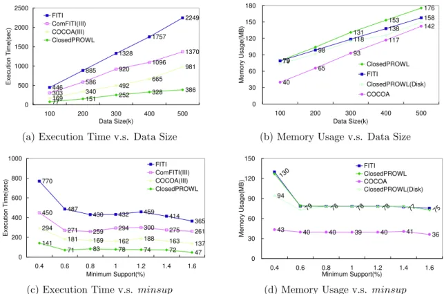
The synthetic data sets which we used for our experiments were generated using the generator described in [2]. We start by looking at the performance of ClosedPROWL with default parameter minsup = 0.6% and maxwin = 5. Figure 1(a) shows the scalability of the algorithms with varying database size. Closed- PROWL is faster than FITI (by a magnitude of 5 for

|D| = 500K). The scaling with database size was lin- ear. Therefore, the scalability of the projected window lists technique is proved. Another remarkable result is that COCOA performs better than ComFITI for the same mining task (compressed frequent continuity mining). The reason for the considerable execution time of FITI and ComFITI is that they must count the sup- ports of all candidate continuities. The memory requirement of the algorithms with varying database size is shown in Figure 1(b). In this case, the number of frequent continuities and closed frequent continuities are 13867 and 1183 respectively. The compression rate (# of closed frequent continuities /# of frequent continuities) is about 9%. As the data size increases, the memory requirement of ClosedPROWL, COCOA and FITI increases as well. However the memory usages of FITI and ClosedPROWL are about the same at |D| = 100K and the difference is only 18MB at |D| = 500K, with an original database of 12.2 MB. Since ClosedPROWL requires additional memory to maintain frequent continuities (F CT ab), we modify the algorithm to disk-resident ClosedPROWL (labelled ClosedPROWL(Disk)). As il- lustrated in Figure 1(b), the memory requirement of the ClosedPROWL(Disk) is thus less than FITI but more

(4)

446 885

1328 1757

2249

303 586

920 ¹⁰⁹⁶

1370

169 ³⁴⁰

492 ⁶⁶⁵

981

77 ¹⁵¹

252 ³²⁸ ³⁸⁶

0 500 1000 1500 2000 2500

100 200 300 400 500

Data Size(k)

Execution Time(sec)

FITI ComFITI(III) COCOA(III) ClosedPROWL

79

131

176

79

98

118

138

158

40

65

93

117 153 142

0 30 60 90 120 150 180

100 200 300 400 500

Data Size(k)

Memory Usage(MB)

ClosedPROWL FITI

ClosedPROWL(Disk) COCOA

(a) Execution Time v.s. Data Size (b) Memory Usage v.s. Data Size

770

487 430 432 ⁴⁵⁹ ₄₁₄

365 450

271 ₂₅₉ ²⁹⁴ ³⁰⁰ 275 ₂₆₁

294

181 ₁₆₉ ₁₆₂ 188 ₁₆₃

141 137

71 ⁸³ 78 74 72 ₄₇

0 200 400 600 800 1000

0.4 0.6 0.8 1 1.2 1.4 1.6

Minimum Support(%)

Execution Time(sec)

FITI ComFITI(III) COCOA(III) ClosedPROWL

13⁰

79 78 78 78 77 ₇₅

43 ₄₀ ₄₀ ₃₉ ₄₀ ₄₁

36 94

0 30 60 90 120 150

0.4 0.6 0.8 1 1.2 1.4 1.6

Minimum Support(%)

Memory Usage(MB)

FITI ClosedPROWL COCOA

ClosedPROWL(Disk)

(c) Execution Time v.s. minsup (d) Memory Usage v.s. minsup Figure 1: Performance comparison I

than COCOA for subitemset pruning (P HT ab). The runtime and memory usage of FITI and Closed- PROWL on the default data set with varying minimum support threshold, minsup, from 0.4% to 1.6% are shown in Figures 1(c) and (d). Clearly, Closed- PROWL is faster and more scalable than both FITI and ComFITI with the same memory requirements (by a magnitude of 5 and 3 for minsup = 0.4% respectively), since the number of frequent continuities grows rapidly as the minsup diminishs. ClosedPROWL and ClosedPROWL(Disk) require 129MB and 94MB at the minsup= 0.4%, respectively. Thus maintaining closed frequent continuities (F CT ab) in ClosedPROWL needs 35MB main memory approximately. Meanwhile, we can observe that the pruning strategies of ClosedPROWL increase the efficiency considerably (by a magnitude of 2) through the comparison between ClosedPROWL and COCOA in Figure 1(c). In summary, projected window list technique is more efficient and more scalable than Apriori-like, FITI and ComFITI, especially when the number of frequent continuities becomes really very large.

4 Conclusion

In this paper, we propose an algorithms for the mining of closed frequent continuities. We show that the three- phase design lets the projected window list technique, which was designed for sequences of events, also appli- cable to general temporal databases. The proposed algorithm uses both vertical and horizontal database formats to reduce the searching time in the mining process. Therefore, there is no candidate generation and multi- pass database scans. The main reason that projected window list technique outperforms FITI/ComFITI is that it utilizes memory for fast computation. This the same reason that later algorithms for association rule mining outperform Apriori. Even so, we have demon- strated that the memory usage of our algorithms are actually more compact than the FITI/ComFITI algorithm. Furthermore, with subitemset pruning and sub- continuity checking, ClosedPROWL successfully discov- ered efficiently all closed continuities. For future work, maintaining and reusing old patterns for incremental mining is an emerging and important research. Fur- thermore, using continuities in prediction is also an in- teresting issue.

(5)

Acknowledgements This work is sponsored by Na- tional Science Council, Taiwan under grant NSC93- 2213-E-008-023.

References

[1] K. Y. Huang and C. H. Chang. Smca: A general model for mining synchronous periodic pattern in temporal database. IEEE Transaction on Knowledge and Data Engineering (TKDE), 2005. To Appear.

[2] K. Y. Huang, C. H. Chang, and K.-Z. Lin. Cocoa: An efficient algorithm for mining inter-transaction associations for temporal database. In Proceedings of 8th European Conference on Principles and Practice of Knowledge Discovery in Databases (PKDD’04), volume 3202 of Lecture Notes in Computer Science, pages 509–511. Springer, 2004.

[3] K. Y. Huang, C. H. Chang, and K.-Z. Lin. Prowl: An efficient frequent continuity mining algorithm on event sequences. In Proceedings of 6th International Confer- ence on Data Warehousing and Knowledge Discovery (DaWak’04), volume 3181 of Lecture Notes in Com- puter Science, pages 351–360. Springer, 2004.

[4] H. Mannila, H. Toivonen, and A. I. Verkamo. Discov- ering frequent episodes in event sequences. Data Min- ing and Knowledge Discovery (DMKD), 1(3):259–289, 1997.

[5] A. K. H. Tung, H. Lu, J. Han, and L. Feng. Ef- ficient mining of intertransaction association rules. IEEE Transactions on Knowledge and Data Engineer- ing (TKDE), 15(1):43–56, 2003.

[6] M. J. Zaki and C. J. Hsiao. Charm: An efficient algorithm for closed itemset mining. In Proceedings of 2nd SIAM International Conference on Data Mining (SIAM 02), pages 457–473, 2002.

Appendix A

Lemma 4.1. _Let _P ₌ _[p₁_{, p}₂, . . . , pw] and Q = [q1, q2, . . . , qw] be two frequent continuities and P.timelist = Q.timelist. For any frequent continuity U , if P · U is frequent, then Q · U is also frequent, vice versa.

Theorem 4.1. _{Let P = [p}₁_{, p}₂, . . . , pw, pw+1] and Q = [p1, p2, . . . , pw, p^′_w+1] be two continuities. If pw+1 ⊂ p^′_w+1 and Sup(P ) = Sup(Q), then all extensions of P must not be closed.

Proof. Since pw+1 is a subset of p^′_w+1, wherever p^′_w+1 occurs, pw+1 occurs. Therefore, P.timelist ⊇ Q.timelist. Since Sup(P ) = Sup(Q), the equal sign holds, i.e. P.timelist = Q.timelist. For any extension P · U of P , there exists Q · U (Lemma 4.1), such that Q · U is a super-continuity of P · U, and (P · U ).timelist = P.P W L|U |^TU.timelist= Q.P W L|U |^TU.timelist= (Q · U ).timelist. Therefore, P· U is not a closed continuity.

Theorem 4.2. _{Let P = [p}₁_{, p}₂, . . . , pw, pw+1] and Q = [p1, p2, . . . , pw, p^′_w+1] be two continuities. If pw+1 ⊂ p^′_w+1 and Sup(P ) = Sup(Q), then all extensions of P must not be closed.

Proof. Consider the continuity U = [p1, p2, . . . , pw, pw+1∪ p^′w+1]. U.timelist=P.timelist^T Q.timelist. Since P.timelist = Q.timelist, we have U.timelist=P.timelist=Q.timelist. Using Theorem 4.2, all extensions of P and Q can not be closed be- cause Sup(U ) = Sup(P ) = Sup(Q).

Appendix B

We also prove the correctness of the ClosedPROWL algorithm below.

Lemma 4.2. The time list of a continuity P = [p1, p2, ...., pw] is P.timelist =^T^w_i=1pi.P W Lw−i.

We define the closure of an itemset p, denoted c(p), as the smallest closed set that contains p. If p is closed, then c(p) = p. By definition, Sup(p) = Sup(c(p)) and p.timelist= c(p).timelist.

Theorem 4.3. A closed continuity is composed of only closed itemsets and don’t care characters.

Proof. Assume P = [p1, p2, . . . , pW] is a closed continuity, and some of the pis are composed of non-closed itemsets. Consider the continuity CP = [c(p1), c(p2), . . . , c(pW)], CP.timelist = Tw

i=1^c(pⁱ^{).P W L}^w−i ⁼

Tw

i=1^pⁱ^{.P W L}^w−i= P.timelist. Therefore, P is not a closed continuity. We thus have a contradiction to the original assumption that P is a closed continuity and thus conclude that “all closed continuities P = [p1, p2, . . . , pW] are composed of only closed itemsets and the don’t-care characters”.

Theorem 4.4. The ClosedPROWL algorithm generates all closed frequent continuities.

Proof. First of all, the anti-monotone property “if a continuity is not frequent, all its super-continuities must be infrequent” is sustained for closed frequent continuities. According to Theorem 4.3, the search space composed of only closed frequent itemset covers all closed frequent continuities. ClosedPROWL’s search is based on a complete set enumeration space. The only branches that are pruned as those that do not have sufficient support. The sub-itemet pruning only removed non-closed continuities (Theorem 4.2). Therefore, ClosedPROWL cor- rectly identifies all closed frequent continuities. On the other hand, sub-continuity checking remove non-closed frequent continuities. Therefore, the ClosedPROWL algorithm generates all and only closed frequent continuities.