Entry by Merger:
Estimates from a Two-Sided Matching Model with Externalities
Kosuke Uetakey Northwestern University
Yasutora Watanabez Northwestern University August 2012
Abstract
As …rms often acquire incumbents to enter a new market, presence of desirable acquisition targets a¤ect both merger and entry decisions simultaneously. We study these decisions jointly by considering a two-sided matching model with externalities to account for the “with whom” decision of merger and to incorporate negative externalities of post-entry competition. By estimating this model using data on commercial banks, we investigate the e¤ect of the entry deregulation by the Riegle-Neal Act. After proposing a deferred acceptance algorithm applicable to the environment with externalities, we exploit the lattice structure of stable allocations to construct moment inequalities that partially identify the banks’ payo¤ function including potential (dis)synergies. We …nd greater synergies between larger and healthier potential entrants and smaller and less-healthy incumbent banks. Compared with de novo entry, entry barriers are much lower for entry by merger. By prohibiting de novo entry, our counterfactual quanti…es the e¤ect of the deregulation.
Keywords: Entry, merger, two-sided matching, partial identi…cation, Riegle-Neal Act
We thank Hiroyuki Adachi, David Besanko, Ivan Canay, Jeremy Fox, John Hat…eld, Marc Henry, Hide Ichimura, Michihiro Kandori, Mike Mazzeo, Aviv Nevo, Rob Porter, Mark Satterthwaite, Matt Shum, Junichi Suzuki, Jeroen Swinkels, Rakesh Vohra, Yosuke Yasuda, and especially Fuhito Kojima, Isa Hafalir, and Elie Tamer, for their valuable comments and suggestions. We also thank Xiaolan Zhou for kindly sharing her data on bank mergers.
yDepartment of Economics, Northwestern University, 2001 Sheridan Road, Evanston, IL 60208. Email: uetake@northwestern.edu
1
Introduction
Firms often use mergers and acquisitions to enter new markets.1 In such cases, presence of desirable acquisition targets a¤ects not only merger decisions but also entry decisions at the same time. For example, a …rm may choose not to enter a market if it cannot …nd a good target incumbent for acquisition. In some markets, entry barriers for de novo entry can be so high that acquiring an incumbent may be the only pro…table way to enter. Thus, entry and merger decisions are joint decisions, and should not be separately studied in those markets. Moreover, as entry by merger impacts the competitive structure of markets, studying entry by merger may have important policy implications.2
In this paper, we study entry and merger decisions jointly in the U.S. commercial banking industry where entry by merger is prevalent. In particular, we investigate the e¤ect of the Riegle-Neal Act (the Act), which deregulated the intra-state de novo entry for 13 states that had not deregulated it at the time of the Act.3 In these 13 states, the legal barrier
for de novo entry was eliminated by the Act in 1997. Using data on bank behavior in the regional markets of these 13 states for the period right after the Act took e¤ect, we study how the Act a¤ected entry and merger decisions.
To study the banks’ behavior, we consider a model in which the “with whom” decision of the merger and the post-entry (and post-merger) competition are addressed simultaneously. We do so by combining a standard entry model (Bresnahan and Reiss, 1991, and Berry, 1992) with a two-sided matching model with contracts (Hat…eld and Milgrom, 2005). For the “with whom” decision, two features are particularly important: i) the payo¤ from merger depends on potential (dis)synergy, which signi…cantly di¤ers across pairs of …rms (we specify a synergy function to quantify potential (dis)synergies), and ii) the merger decision is not a unilateral one because the target …rm must agree to the merger contract. Re‡ecting these features, we adopt a matching model. Speci…cally, we consider a one-to-one two-sided matching model in which …rms are partitioned into two sides, incumbents (I) and
1A signi…cant fraction of market entry is reported to be by merger. Yip (1982) reported that more than one-third of entries in 31 product markets in the United States over the period 1972-1979 were by acquisition. Among 558 market entries into the United States by Japanese companies during 1981-1989, Hennart and Park (1993) found that entry by merger accounted for more than 36%.
2Enty by merger has been an important antitrust issues. The Federal Trade Commission (FTC) explicitly considers “potential new competitors” in its Merger Guidelines. A classic case is the FTC’s decline of a merger attempt by Procter & Gamble (P&G) and the Crolox Corporation in 1967. FTC argued that P&G was the most likely potential entrant in the household bleach industry, and that P&G’s acquisition of Clorox would eliminate P&G as a potential competitor, which would substantially reduce the competitiveness of the industry.
potential entrants (E), because the vast majority of the mergers in our data are mergers between one incumbent and one potential entrant.4
Regarding how we incorporate the e¤ect of post-entry competition into the matching model, we follow a standard entry model (Bresnahan and Reiss, 1991, and Berry, 1992) in which the e¤ect of competition on pro…t is modeled as a decreasing function of the number of operating …rms. Considering this e¤ect of competition on pro…t (negative externalities), a …rm chooses the best option out of the three types of optionsfEnter with merger, Enter without merger, Do not enterg.5 Because the pro…t of a …rm depends not only on the
…rm’s matching (merger partner) but also on the merger and entry decisions of other …rms (e.g., whether another incumbent is acquired by a potential entrant), the model we consider becomes a two-sided matching modelwith externalities.
Considering externalities in a matching model poses a challenge (see, e.g., Sasaki and Toda, 1996, and Hafalir, 2008). This is because, with externalities, payo¤s depend not only on matching but also on the entire assignment of who match with whom. The solution concept in such a case thus has to take into consideration, for each deviation, what the entire assignment would be in addition to with whom the deviating players would match. To incorporate what the assignment would be after each deviation, Sasaki and Toda (1996) and Hafalir (2008) propose anestimation function that maps each deviation to an expectation about the possible assignments following the deviation. Despite taking this approach, the model with general form of externalities is complex and the existence of a stable matching requires strong conditions. In our case, however, complexities are reduced by the fact that the externalities take a particular form — it depends only on the aggregate number of operating …rms negatively (i.e., negative network externalities). Hence, we can modify the estimation function approach so that the estimation is only about the aggregate number of operating …rms.
As we incorporate externalities, the de…nition of stability as a solution concept has to be modi…ed accordingly. In addition to the regular de…nition of stability (i.e., individual rationality and no-blocking-pair condition), we require what we call consistency of esti-mation: The estimated number of operating …rms should be consistent with the actual number of operating …rms. Because we can show that the number of actual operating …rms is decreasing function of the estimated number of operating …rms (i.e., as the estimation on the number of operating …rms increases, less …rms have incentive to enter.), we can prove
4This fact re‡ects the types of market we observe: our data is from small regional markets where average number of incumbents are less than 5 (see Section 3 for the detail), thus mergers between incumbents or mergers involving more than two incumbents tend to be infeasible due to antitrust concerns.
the existence of a solution. We do so by proposing a generalized Gale-Shapley algorithm with externalities. The algorithm is a nested …xed point algorithm that has Hat…eld and Milgrom’s (2005) generalized Gale-Shapley algorithm as an inner loop conditional on the estimated number of operating …rms in the market. The outer loop searches for the …xed point of the estimated number of operating …rms so that it satis…es the consistency of estimation.6
Another challenge is an econometric one: the model has multiple equilibria and the parameter cannot be point-identi…ed without imposing some equilibrium selection rules. Instead of imposing equilibrium selection rules, we take the partial-identi…cation approach exploiting the lattice property of the equilibrium. Though the econometrician cannot tell which equilibrium is played in the observed data, the equilibrium characterization provides upper and lower bounds for the equilibrium payo¤s for each …rm. To be more precise, all incumbents have the highest equilibrium payo¤ in incumbent(I)-optimal equilibrium, and the lowest equilibrium payo¤ in potential entrant(E)-optimal equilibrium. All other equilibrium payo¤s are bounded by these two. Hence, the payo¤ corresponding to the observed outcome is bounded above and below by these extremum equilibrium payo¤s, from which we construct moment inequalities for incumbents. Similarly, all potential entrants obtain the highest payo¤ in E-optimal equilibrium and so on. Thus, we can construct moment inequalities using these equilibrium characterizations without the knowledge of the equilibrium selection rule.
The identi…ed set can be reduced further by considering other equilibrium properties on top of the moment inequalities in payo¤s. In all equilibria, the model predicts a unique number of operating …rms and a unique number of mergers (the result is analogous to the
lone wolf theorem and the rural hospitals theorem. See, e.g., Roth, 1986, and Hat…eld and Milgrom, 2005). Using these properties, we construct moment equalities on the number of operating …rms in addition to the moment inequalities on payo¤s.
Identi…cation of the model, including the identi…cation of the synergy function, is ob-tained by two types of exclusion restrictions. The …rst type of exclusion restriction is a standard one used in the entry model literature following Berry (1992) and Ciliberto and Tamer (2009): we consider a variable that a¤ects a …rm’s own payo¤ but not the other …rms’ pro…ts. The second type of exclusion restriction takes advantage of match-speci…c characteristics: we consider a variable that in‡uences only the (dis)synergy between the pair of …rms, but do not in‡uence the pro…ts of the …rms of the pair if they enter without merger and the (dis)synergy of any other combination of …rms. Using the second exclusion
restriction, we can make any merger to be less attractive than not entering. Then, the model become equivalent to the regular entry model because entering without merger and not entering are the only viable choices in such cases. Thus, we can use the …rst exclusion restriction to identify payo¤s for entering without merger in the same way as the regular entry model is identi…ed. Now, given the payo¤ of entering without merger is identi…ed, the synergy function can be identi…ed from the variations in merger probabilities and in …rm characteristics.
Based on the moment equalities and inequalities discussed above, we estimate the model using Andrews and Soares’s (2010) generalized moment selection. In computing the sample analogue of the moments, we run the generalized Gale-Shapley algorithm with externalities in order to obtain both I-optimal and E-optimal equilibria for each simulation draw for each market.
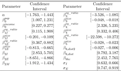
We …nd a signi…cant di¤erence in entry barriers for incumbents, potential entrants, and entry by merger. The entry barrier for potential entrants is much higher than that of the incumbents as well as that of entry by merger, causing a signi…cant fraction of entry by potential entrants to take the form of merger and acquisition. Concerning the (dis)synergies from mergers between di¤erent types of …rms, bank characteristics a¤ect (dis)synergy di¤erently across the sides of incumbents and potential entrants. We …nd that synergy between potential entrants with a larger asset size and higher equity ratio and incumbents with a lower equity ratio tends to be much higher. This may re‡ect the pattern in the data that large and healthy banks enter new markets by buying incumbents with less-healthy balance sheets.
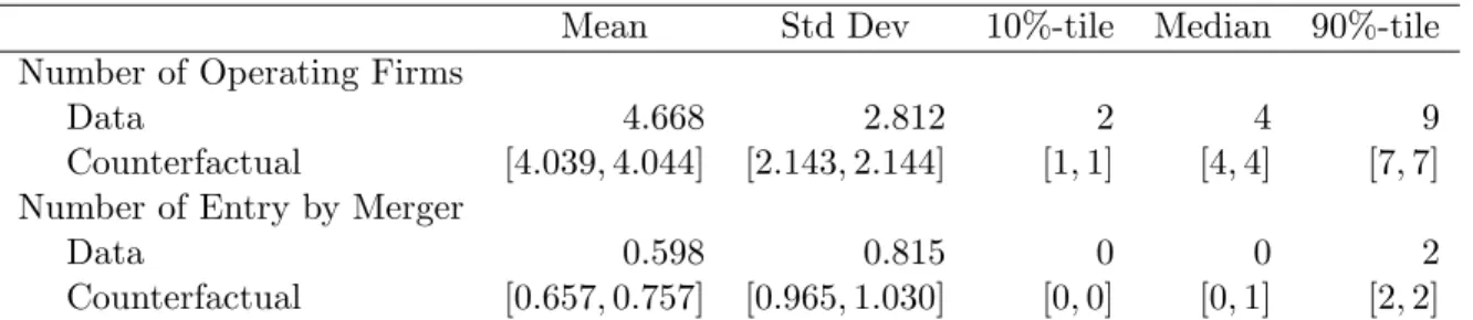
Finally, we conduct a counterfactual policy experiment to assess the e¤ect of the Act. We …nd the number of banks operating in a market would have decreased if de novo entry by potential entrants had not been deregulated by the Act. Prohibition of de novo entry provides stronger incentive to enter by merger for potential entrants, and accordingly we …nd that the number of entry by merger increases if de novo entry were prohibited.
In the rest of the paper, we present a two-sided matching model in Section 2 after discussing the related literature in Section 1.1. All proofs for Section 2 are in Appendix A. We document the data in Section 3, and then provide the econometric speci…cation, identi…cation, and estimation procedure in Section 4. Section 5 reports the results of the estimation and the counterfactual experiment. Finally, we conclude in Section 6.
1.1 Related Literature
a new approach to estimate a matching model with non-transferrable utility.7 Only a few
papers estimate matching models with non-transferrable utility. Gordon and Knight (2009) consider merger of school districts, and their speci…cation on match quality is similar to our synergy function, though they consider a one-sided matching model (roommate problem). Also their paper is close to ours as they run an algorithm to …nd a stable matching in their estimation. Sorensen (2007) studies the matching between venture capitalists and entrepreneurs, and estimates the model under the assumption that players have aligned preferences. Boyd et al. (forthcoming) similarly estimate a two-sided matching model between teachers and schools by running the Gale-Shapley algorithm with the assumption that the school-optimal stable matching is realized. Similarly with a known equilibrium selection mechanism, Uetake and Watanabe (2012) propose another estimation strategy for a two-sided matching model with non-transferable utility using Adachi’s (2000) prematching mapping. In environments with only aggregate-level data available, Echenique, Lee, Shum, and Yenmez (forthcoming) study testable implications of stable matchings. In a similar environment, Hsieh (2011) proposes a modi…ed deferred acceptance algorithm to study identi…cation and estimation. These two papers di¤ers from ours as they consider aggregate-level data while we use individual-aggregate-level data. Our paper also di¤ers from these papers in that we consider matching with contracts. Finally, a number of papers estimate matching models with transferrable utility.8 Among these, Akkus and Hortaçsu (2007) and Park (2011) are close to ours in that they study the merger of banks and mutual funds, respectively. Our paper adds to these papers by explicitly considering the e¤ect of post-merger competition. The second strand of the related literature is the large and growing theoretical literature on matching.9 Our paper builds on Hat…eld and Milgrom (2005, hereafter denoted as HM), who study a matching model with contract. In fact, our theoretical characterization is derived using the nested …xed-point algorithm, which contains HM’s generalized Gale-Shapley algorithm as the inner loop. HM characterize the set of stable allocations for the matching model with contract. HM show that the set of stable allocations in two-sided matching with contracts has lattice property and proves the existence using Tarski’s …xed-point theorem.10 We follow their approach and incorporate two additional features; we
allow externalities and participation decisions. In matching models, a player’s individual rationality condition is about whether he has incentive to be matched with others, but not about his participation to the matching market. We explicitly consider the incentive to
7Although there is a transfer, our model is a model with non-transferrable utility. This is because players do not value transfers in the same way.
8See, e.g., Choo and Siow (2006), Fox (2010), Galichon and Salanié (2010), Bacarraet al. (2012), and Chiappori, Salanié, and Weiss (2010) .
9See, e.g., a survey by Roth (2008).
“participate,” and make the preference dependent on the number of “participants,” which is the externalities we consider.
To the best of our knowledge, Sasaki and Toda (1996) and Hafalir (2008) are the only papers that investigate a two-sided matching model with externalities. Both papers consider a very general form of externalities. Analyzing such matching models is di¢cult because preference is de…ned over the set of assignments rather than matchings. Hence, regular de…nition of “stability” or “deviation” are not su¢cient to analyze such a model because a deviating pair’s preference also depends on how other agents would react to their deviation, not just their matching. To model how other agents would react to a player’s deviation, both papers use what they call the estimation function approach. Estimation functions specify the expectations on the assignment (i.e., what the matching among all players would be) after each deviation. They prove that a strong requirement on the estimation function is necessary in order to guarantee the existence of stable matching. Based on their estimation function approach while considering a particular form of externalities (the payo¤ depends only on the number of operating …rms in the market), we show the existence and provide characterizations.
The third strand of the literature is the literature on estimating entry models following Bresnahan and Reiss (1991) and Berry (1992), where the …rms’ underlying pro…t functions are inferred from the observed entry decisions.11 We add to this literature by examining the entry and merger decisions jointly. We do so by combining two-sided matching model with the entry model. Our approach is similar to Ciliberto and Tamer (2009) in using a set estimator to address multiplicity of equilibria. Also, our identi…cation argument builds on their identi…cation results. Complementary to our study, Perez-Saiz (2012) considers a similar question and adopts an extensive form game for the merger and entry process in the U.S. cement industry. He models merger decisions to be conditional on entry decisions, while these decisions are joint decisions in our model. Other related studies include Jia (2008) and Nishida (2012) that characterize the equilibrium of an entry model with correlated markets as a …xed point in lattice and solve for it to estimate the model. Our paper di¤ers from theirs in that ours make no equilibrium selection assumption and construct moment inequalities exploiting the lattice properties.
The fourth strand is the literature on horizontal merger decisions. In spite of the large literature considering the e¤ects of mergers, studies on the endogenous horizontal merger decision itself are limited.12 Kamien and Zang (1990) show limits to monopolization through mergers, and Qiu and Zhou (2007) point out the importance of …rm heterogeneity in horizon-tal mergers. Gowrisankaran (1999) develops a computable dynamic industry competition
1 1Other recent contributions include Mazzeo (2002) and Seim (2006).
model with an endogenous merger decision. Pesendorfer (2005) …nds the relationship be-tween market concentration and the pro…tability of mergers using a repeated game with merger decision. In a model with de novo foreign direct investment and cross-border merger and acquisitions, Nocke and Yeaple (2007) show the importance of …rm heterogeneity as key determinants. Our paper adds to this literature by empirically investigating the role of …rm heterogeneity in merger decisions.
Finally, our paper is also related to the literature studying banks’ branching decisions. Ru¤er and Holcomb (2001) use data from California and investigate the determinants of a bank’s expansion decision by building a new branch and acquiring an existing branch, respectively. Their results show that a large bank would be likely to enter a new market by acquisition, but not through building a new branch, which is consistent with our result that larger potential entrants have higher synergy ceteris paribus. Wheelock and Wilson (2000) study the determinants of bank failures and acquisitions using a competing-risks model. Consistent with our …nding, they show that less capitalized banks are more likely to be acquired for the period between 1984 and 1993. Cohen and Mazzeo (2007) estimate an entry model with vertical di¤erentiation among retail depository institutions, and …nd evidence of product di¤erentiation depending on market geography.
2
Model
We model the entry and merger decisions as a two-sided matching problem with externali-ties. We build the model combining models of entry (Bresnahan and Reiss, 1991, and Berry, 1992) and two-sided matching with contracts (Hat…eld and Milgrom, 2005). After describ-ing the model, we propose the solution concept that addresses externalities, N-stability. Then, we provide characterizations of theN-stable outcomes: the set ofN-stable outcomes forms a complete lattice, and the two extremum points of the set can be obtained by run-ning a deferred acceptance algorithm that we propose. We use these characterizations for identi…cation and estimation of the model.
2.1 A Matching Model of Entry and Merger
We consider a static entry model in which …rms can use merger and acquisition as a form of entry in addition to regular entry without merger. In particular we integrate entry and merger decisions into a two-sided matching model between an incumbent …rm (denoted by
We adopt a two-sided matching model because mutual consent between the two parties is required for a merger. In particular, we consider one-to-one two-sided matching instead of coalition formation, one-to-many matching, or many-to-many matching for the reason that the vast majority of mergers in our data are one-to-one mergers between an incumbent and a potential entrant. This fact re‡ects the types of market we observe: our data is from small regional markets where average number of incumbents are less than 5 (see Section 3 for the detail), thus mergers between incumbents or mergers involving more than two incumbents tend to be infeasible due to antitrust concerns. Finally, we consider a matching model instead of a speci…c extensive form game because the details about individual merger process (such as how investment banks and FDIC are involved in each case, how both sides negotiate the merger contract, etc.) are not observable in general.
Our matching model adds two features to a regular two-sided one-to-one matching model with contracts by i) considering two outside options (the decisions of “enter without merger” and “not to enter”), and ii) incorporating externalities that depend on the number of oper-ating …rms (network externalities).
Firms on both sides have three types of choices. Potential entrant ecan choose not to enter (denoted by fog), enter by itself (denoted by feg), or merge with incumbent i with a merger contract kei (denoted by fkeig). Merger contracts are bilateral ones between a
potential entrant and an incumbent, and each …rm can sign only one merger contract with a …rm on the other side. A contract kei = (e; i; pei) speci…es a potential entrant and an
incumbent pair and the terms of the merger, pei 2P, where the set of merger terms P is
…nite as in HM.
Similarly to potential entrants, incumbentihas three types of choices: it can choose not to enter (denoted byfog), enter by itself (denoted by fig), or merge with potential entrant
ewith a merger contract kei (denoted by fkeig).
We denote the set of merger contracts by K E I P. Note that the set of merger contracts does not include the case where a potential entrant or incumbent does not enter the market or the case where they enter by themselves. Let the set of merger contracts in which entranteis involved be Ke and in which incumbentiis involved be Ki, i.e.,
Ke=
[
i2Ifkeig, and Ki=
[
e2Efkeig: We also de…ne the set of available choices foreand ias
Ke=Ke[ feg [ fog and Ki =Ki[ fig [ fog:
For simplifying the notation, we de…ne K= [
j2E[I
Payo¤s depend on the outcome of the matching game. Because we consider entry and merger decisions after which …rms compete, a …rm’s payo¤ is a¤ected not only by its entry and merger decisions but also by other …rms’ entry and merger decisions. Hence, we need to consider a model with externalities due to post-entry competition. To address these externalities, we follow Bresnahan and Reiss (1991) and Berry (1992) and assume that the number of operating …rms,N, negatively a¤ects the payo¤ of the …rm (note thatN depends on entry and merger decisions jointly). Furthermore, as non-monetary components such as a manager’s idiosyncratic taste over the potential merger may play an important role in the actual merger decisions, e.g., Malmendier and Tate, 2008), we allow the payo¤ of a …rm to depend not only on the pro…t but also on other factors. We denote the payo¤ of incumbent
ias
i(kei; N) = 1i i(kei; N) +"ei i(i; N) = 1
i i(i; N) +"ii
i(o; N) = 0
if …rmimerges with …rm ewith contractkei,
if …rmienters without merger,(se
if …rmidoes not enter,
where i(; N) is the monetary pro…t with N operating …rms, "ei and "ii are idiosyncratic
shocks, and i is a parameter that captures the relative importance of idiosyncratic shocks
to the monetary pro…t. Re‡ecting the negative externalities of the post-entry competition as in the empirical entry literature, we assume i(k; N)< i(k; N 1)for allk2Ki[ fig.
Also, as we assume "ei and "ee to be continuously distributed, the preferences are strict
generically.
In the same way, we can write potential entrant e’s payo¤ as
e(kei; N) = 1e e(kei; N) +"ie e(e; N) = 1e e(e; N) +"ee e(o; N) = 0
if …rme merges with …rmiwith contract kei,
if …rme enters without merger, if …rme does not enter,
where e(; N)is the monetary pro…t withN operating …rms,"ei(6="ie) and"eeare
idiosyn-cratic shocks, and e is a parameter that captures the relative importance of idiosyncratic
shocks. We do not impose "ei = "ie since acquiring and target …rms may have
heteroge-nous preferences on the potential merger. As in the case of the incumbents, we assume
e(k; N)< e(k; N 1)for all k2Ke[ feg, and preferences are strict generically.
Note that the model is a matching model with non-transferable utility, though the terms of the merger contract may include transfers between the …rms. This is because we allow i and e to be di¤erent across …rms, re‡ecting the fact that factors not directly
and shareholder interests are misaligned as in Jensen and Meckling (1976). Other sources could be di¤erences in CEOs’ overcon…dence on merger decisions (Malmendier and Tate, 2008) and variations in manager’s strategic ability on entry decisions (Goldfarb and Xiao, 2011).
2.2 Solution Concept: N-Stable Outcome
2.2.1 Estimation Function and Chosen Set
We extend the solution concept of stable allocation of Hat…eld and Milgrom (2005) to our environment with externalities. Considering externalities in two-sided matching is di¢cult in general (Sasaki and Toda, 1996, Hafalir, 2008). This is because preference is dependent not only on one’s own matching (as in the case without externalities), but also on how other players are matched with each other (i.e., the entire assignment). This dependence of preference on the entire assignment requires us to consider how players expect the reaction of other players in thinking about the de…nition of stability that is appropriate for the matching model with externalities.
In order to describe the way each player expects how other players are matched with each other, we follow Sasaki and Toda (1996) and Hafalir (2008) to use theestimation function
approach. In a matching model with externalities, if a pair of players deviates (dissolves the match), each member of the pair has to think not only about their own matching but also about how other players (including his/her previous partner) are reacting to the deviation because preferences are de…ned over assignment rather than matching.13 Sasaki
and Toda (1996) and Hafalir (2008) de…ne the estimation function as a mapping from the set of possible matches to the set of matchings of all players, which speci…es the expected assignments resulting from a deviation. In our notation, the estimation function of …rm j, denoted by Nj, isNj :Kj ! K if we consider a general form of externalities.
In our environment, however, we focus on the (network) externalities that enter into the …rm’s payo¤ only through the number of operating …rms in the market, N (note that this depends on the outcome of matchings of other …rms as well).14 Thus, we de…ne the estimation function for …rm j as Nj : Kj ! R+, a mapping from the possible choices to
1 3To illustrate this point, suppose Players A and X are currently matched. If Player A deviates to form a blocking pair with Player Y, Player A has to consider not only that Player Y has incentive to be matched with A, but also what other players, including Player X, would do after the deviation, because the entire outcome (rather than just whom Player A is matched with) a¤ects Player A. Thus, Player A’s expectations about the possible entire outcomes after the deviation are crucial.
1 4This assumption can be relaxed in some dimensions such as the case that the …rms are vertically di¤erentiated as in Mazzeo (2002). Suppose each …rm has its type based on some observable …rm speci…c characteristics such as high, medium, and low quality or for- and non-pro…t. Denote the number of total operating …rms for each type byNs; s = 1;2; :::; S. Then, the payo¤ can depend on the total number of operating …rms for eachtype: j(fkg;(Ns)S
theestimated number of operating …rms.15 For example,N
e(e) = 3denotes that potential
entrant e estimates the number of operating …rms to be 3 ife enters the market without merger, and the function Ne( ) speci…es the estimated number of operating …rms for all
other possible choicesoandkei as well, such asNe(o) = 2and Ne(kei) = 5. This restriction
on the form of externalities allows analysis and characterization to be more tractable than those of existing works.
Now we describe the choice by …rms given the estimation function. In order to represent the choice by a potential entrant given the set of available merger contracts Ke and the
estimation functionNe, we de…ne thechosen set from merger contracts Ce(Ke;Ne)foreas
the following:
Ce(Ke;Ne) =
(
?if maxf e(o;Ne); e(e;Ne)g maxk2Kef e(k;Ne)g
kei if e(kei;Ne) e(k;Ne); 8k2Ke;
where e(k;Ne) e(k;Ne(k))by suppressing kfromNe(k). This set is the best available
merger contract given the available set of contractsKe, which can be a null set if no merger
contract is more attractive than de novo entry and no entry. Similarly, we de…ne the chosen set from merger contracts for incumbentigiven the available set of contractsKi as follows:
Ci(Ki;Ni) =
(
?if maxf i(o;Ni); i(i;Ni)g maxk2Kif i(k;Ni)g
kei if i(kei;Ni) i(k;Ni); 8k2Ki;
which also can be a null set if no merger contract is more attractive than de novo entry and no entry.
In addition to the chosen set from merger contracts, we also need to track the choice of …rms including no entry and entry without merger. We denote thechosen set for incumbent
ibyCi(Ki;Ni)and for potential entrantebyCe(Ke;Ne), which is either the most preferred
merger contract available to …rm j inKj, entry without merger, or no entry, i.e.,
Ci(Ki;Ni) = argmaxk2Kif i(k;Ni)g;
Ce(Ke;Ne) = argmaxk2Kef e(k;Ne)g:
The di¤erence between the chosen set from merger contracts and the chosen set is that
Ci(K;Ni)andCe(K;Ne)take the null set if any merger contract inK is not preferred to no
entry or entry without merger, whileCi(Ki;Ni) andCe(Ke;Ne)specify the optimal choice
among Kj for each player, which may include no entry or entry without merger.
2.2.2 N-Stability
In matching models without externalities, a matching is stable if it satis…es i) the no-blocking-pair condition and ii) individual rationality. The no-no-blocking-pair condition re-quires that there be no pair of players who are weakly better o¤ than they would be with their current match. Individual rationality requires that no player form a couple that is less preferable than being unmatched. Our version of stability adds to the standard de…nition of stability in two ways. First, to address the issue resulting from the presence of external-ities, we modify the solution concept of '-stability in Sasaki and Toda (1996) and Hafalir (2008).16 Second, we slightly modify the individual rationality so that …rms can choose to be unmatched in two ways: …rms can choose “not to enter the market” (fog) or “to enter the market without merger” (figand feg).
Externalities require an additional condition on the regular solution concept of stability because the players have anestimation functionabout what might happen after each choice, and the behavior of players needs to be consistent with the estimation function. Sasaki and Toda (1996) and Hafalir (2008) call this condition '-admissibility. They use this condition to de…ne their solution concept for matching models with externalities (called '-stability). We follow their approach and consider a solution concept that incorporates our estimation functionN discussed above (our estimation function is simpler than theirs), which we call N-stability.
The way we incorporate the estimation functionN to our solution concept is by requiring the “consistency” of the estimation function, i.e., each …rm’s estimation on the number of operating …rms equals the actual number of operating …rms. In order to de…ne consistency, let us …rst de…ne correspondence , which maps from the set of all the …rms’ estimation functions and the set of available contracts to positive real numbers. This correspondence, , computes the resulting number of operating …rms given the chosen set of all players and estimation functionN =fNjgj2E[I, i.e.,
(K;N) = 1 2
2
4NE+NI
X
j2E[I
pj(o;K;Nj) +
X
j2E[I
pj(j;K;Nj)
3 5;
wherepj(k;Kj;Nj) is a probability distribution over the setCj(Kj;Nj) de…ned as follows:
pj(k;Kj;Nj) =
8 > < > :
1
qk
0
iffkg=Cj(Kj;Nj)
ifk2Cj(Kj;Nj) and fkg 6=Cj(Kj;Nj)
ifk =2Cj(Kj;Nj)
;
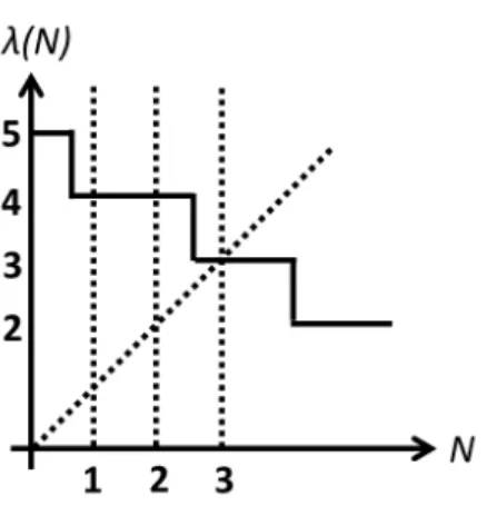
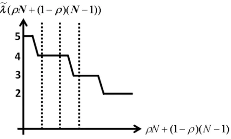
Figure 1: An example of (K; N) for a given K (we suppress the dependence on K). N
is estimation on number of entering …rms, and (K; N)is the resulting number of entering …rms given estimationN. We show that (K; N)is decreasing inN in Lemma 1. 45-degree line corresponds to consistency of estimation.
where P 2C
j(Kj;Nj)q = 1 with q 2 [0;1]. The correspondence simply returns the number of operating …rms. Figure 1 presents an example of . Note that we usepj(o;K;Nj)
instead of 1 Cj(K;Nj) =o to allow for mixing of choices by the players in a nongeneric
case when Cj(Kj;Nj) is not a singleton (i.e., fkg 6= Cj(Kj;Nj)). Such non-generic case
may occur if a …rm is indi¤erent between alternatives. For a generic case that the chosen set is singleton (i.e.,fkg=Cj(Kj;Nj)), the choice probability for the alternative is 1. As the
correspondence aggregates choice probabilities of each …rm, these imply that the range of
(; ) is R+:
We allow mixing of choices by a player in a nongeneric case of indi¤erence in order to guarantee the existence of a solution.17 Indi¤erence occurs, for example, in a nongeneric case where a …rm’s pro…t from entering alone happens to be zero. Such cases occur for some speci…c values ofN, corresponding to the vertical jump of (K; N)in Figure 1 where
(K; N) takes a set value between two integers. In such a case, we consider that the …rm may mix between the indi¤erent choice alternatives with probabilityqk fork2Cj(Kj;Nj).
This implies that is in fact a correspondence (becauseqkcan take any value withqk2[0;1]
and P 2C
j(Kj;Nj)q = 1 ), which we later use to apply Kakutani’s Fixed Point Theorem to guarantee existence of the solution as discussed further in Section 3.2.
1 7Note that the discreteness is one of the reasons why guaranteeing existence of stable matching is di¢cult in general when externalities are present. In our case, we approach this di¢cutly by relying on the fact the indi¤erence occurs in a particular way as described (and thus we allow for mixing), so that we can show existence and characterize the stable outcome.
Now we can write the consistency requirement: the set of available choices K and estimation function N are such that the number of operating …rms equals the estimated
number of …rms, i.e.,
Condition 1 (Consistency of Estimation) A set of available choices and estimation function(K;N) is consistent if
Nj(kj)2 (K;N); 8j 2 E [ I;
where kj 2Cj(K;Nj).
In Figure 1, this condition corresponds to the point on 45-degree line where intersects. This is because the estimated number of operating …rm equals the resulting number of operating …rms.
The second modi…cation to the standard de…nition of stability is that we allow two out-side options: entry without merger and no entry. In the standard de…nition of individual rationality for matching models, players compare being unmatched to matching with some-one. In such cases players can unilaterally choose to stay in the market alsome-one. In our case, the players choose one of the better outside options if they were not matched, and they can make this decision unilaterally. We write this condition as follows18:
Condition 2 (Individual Rationality) A set of available choices and estimation func-tions (K;N) is individually rational if 8j 2 E [ I;@ek2Kj s.t.
j(ek;Nj) j(Cj(K;Nj);Nj).
The last condition we require is theno-blocking-contract condition. It requires that there exist no merger contracts to which …rms from both sides would be willing to deviate. This condition is a standard one to de…ne stability in a two-sided matching model with contracts (see, e.g., HM). To de…ne this condition, let us …rst de…ne the set of merger contracts included in the set of outcomes K by K, i.e.,K =Sj2E[IKjn(fog [ fjg). This is simply
the set of merger contracts chosen given K. Using this notation, the no-blocking-contract condition can be written as follows:
Condition 3 (No Blocking Contracts) A set of available choices and estimation func-tions (K;N) admits no blocking contracts if @ek K s.t. ek6=K and
e k=[
i2ICi(K[ek;Ni) =
[
e2ECe(K[ek;Ne).
Now we de…ne our solution concept of N-stabile outcome using the three conditions de…ned above.
De…nition 1 (N-stable outcome) A set of available choices and estimation functions (K ;N ) is a N-stable outcome if Conditions 1,2, and 3 are satis…ed.
In the next section, we propose a deferred acceptance algorithm, which accommodates externalities in order to show the existence of N-stable outcomes, and provide characteri-zations. We use those characterizations as the basis of our estimation strategy.
2.3 A Generalized Gale-Shapley Algorithm with Externalities
In this section, we show the existence of N-stable outcome by proposing a generalized Gale-Shapley algorithm with externalities, and also show some of the properties of the N-stable outcome, which we use for our identi…cation and estimation. The algorithm we propose uses HM’s generalized Gale-Shapley algorithm as an inner loop conditional on the estimated number of …rms. The outer-loop adjusts …rms’ estimation in order to …nd the estimated number of operating …rms,N , such that it equals the actual number of operating …rms, i.e., satisfying the Consistency of Estimation, N =Nj(kj)2 (K ;N ) (Condition
1).
First, we consider an estimation functionN that is part of the de…nition of theN-stable outcome. We use the following estimation function: 8j2 E [ I,8k2Kj,
Nj(k) =N,
for some N < NE +NI.19 This describes that the number of estimated operating …rms remains unchanged by …rm j’s choice k. In other words, there are certain number of …rms that the market can accommodate, and …rm j’s choice does not a¤ect this number. Note that this estimation function does not exclude the case of other …rms changing their behavior.20
1 9Note that we do not allowN =N
E+NI for the reason that there always exist some potential entrants that do not enter in our data.
2 0Baccara et al.(2012) also consider matching with externalities, and they assume that player’s behavior does not change after any deviation. Using estimation function approach, their assumption in our context can be described as follows:
Nj(k) =
8
<
:
N ifk=j N 1ifk=kjl
N 1ifk=o.
Note that this estimation function does not necessarily imply their assumption (while their assumption implies this estimation function). This is because the above estimation function only concerns theaggregate
One property related toN plays an important role for us to show existence through our algorithm: the number of operating …rms given estimation N is weakly decreasing in N. This property is directly driven by the property that the payo¤ of the …rms negatively de-pends onN. Because is a correspondence, we de…ne function min(K;N) min (K;N)
and max(K;N) max (K;N), which are simply functions that take the minimum and maximum values of the correspondence (K;N), to illustrate this property.
Lemma 1 Given the estimation function Nj(k) = N; 8k 2 K, the functions min(K;N)
and max(K;N) are weakly decreasing in N. Also, (K;N) is upper-hemicontinuous.
All the proofs are in Appendix A. This Lemma implies that as the estimation becomes optimistic (with a small number of operating …rms), the number of …rms that actually enter increases, and vice versa. This property, combined with HM’s generalized Gale-Shapley algorithm, yields a …xed point forN using the algorithm we propose below.
Our algorithm is a nested …xed-point algorithm that consists of inner and outer loops. The inner loop is a variation of HM’s generalized Gale-Shapley algorithm conditional on an estimated number of …rms, and the outer loop is a simple minimization algorithm that runs to …nd a …xed point corresponding to the consistency of estimation (Condition 1).
A Generalized Gale-Shapley Algorithm with Externalities
1. (Outer Loop) Set N = 0 as an initial value forN:Use any minimization routine21 to
minimize min(K; N) N .
2. (Inner Loop) Run the following (E-proposing) generalized Gale-Shapley algorithm given N:
(a) Initialize KE =K,KI =?:
(b) All e2 E choose feg;fog, or make the o¤er that is most favorable to efrom KE to members of I.
(c) Alli2 I considerfig;fog, and all available o¤ers, then hold the best, and reject the others.
(d) UpdateKE by removing o¤ers that have been rejected. UpdateKI by including newly made o¤ers.
deviations. We provide the existence result and an algorithm to …nd a stable outcome for this estimation function in the Supplementary Material. The idea is to combine the generalized Gale-Shapley algorithm with externalities we propose and the EM algorithm for the distribution of players with di¤erent types of estimations.
2 1Because min(K; N) N is quasiconvex in N, global minima can easily be obtained by any
(e) If there is no change to KE and KI, count the number of operating …rms
min(K
E\KI; N) and go to Step 3. Otherwise, return to Step (b).
3. (Outer Loop) If the convergence criterion of the minimization routine is not satis…ed, obtain N for the next round from the minimization routine, and go to step 2. If the convergence criterion of the minimization is satis…ed, terminate the algorithm.
We can also consider I-proposing algorithm, which would entail making the following changes to Step 2 above: substituting KI =K, KE =? with KE = K, KI = ? in (a); e withiin (b); iwith ein (c); and KE with KI andKI with KE in (d).
The inner loop of our algorithm corresponds to HM’s generalized Gale-Shapley algorithm because the estimation ofN is …xed. In each round each potential entrant o¤ers a merger contract to an incumbent or chooses either of the outside options in step (b), and each incumbent holds the best contract o¤ered or either of the outside options in step (c). The set of available contracts forI,KI, starts with an empty set and expandsmonotonically as more o¤ers are (cumulatively) made each round. The set of available contracts for E,KE, starts with the entire set of contracts in step (a), and itmonotonically shrinks as o¤ers are rejected each round. HM show the existence of stable allocation and the characterization using this (inner-loop) algorithm as follows.
Theorem 1 (Hat…eld and Milgrom (2005)) (i) The E-proposing inner loop converges to the E-optimal stable allocation given N, K E(N), and the I-proposing inner loop con-verges to the I-optimal stable allocation given N,K I(N);
(ii) The set of stable contractsK E(N)is unanimously the most preferred set of contracts among all of stable contracts forE and unanimously the least preferred forI, and vice versa for K I(N);
(iii) The number of operating …rms (K; N) is the same for all stable allocations given
N;
(iv) An unmatched …rm in a stable allocation is also unmatched in any stable allocation given N:
Parts (iii) and (iv) of Theorem 1 are the so-called “rural hospitals theorem” (Roth, 1986). In our case, this indicates that the set of …rms that are unmatched is the same for all stable outcomes,22 which in turn implies that the number of operating …rms, (K;N), is
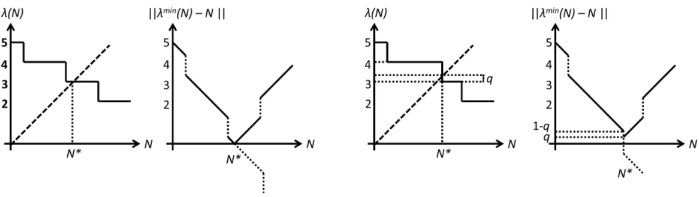
Figure 2: Finding consistent N. The two pictures on the left correspond to the case whereN is an integer. The two pictures on the right correspond to the case where there is mixing, with probabilityq. The function min(K; N) N is quasi-concave, and converges globally toN by applying any regular minimization alogorithm. In the …gure, we suppress the dependence of min on K.
the same for all stable outcomes givenN.23 Thus, (K;N)is the same in bothE-proposing
and I-proposing algorithms.
Given this property of the inner loop, the outer loop of our algorithm …nds the estimated number of operating …rms N satisfying the consistency condition, N 2 (K;N). The following proposition shows there exists suchN.
Proposition 1 There exists N such that N 2 (K ;N ).
Now, using Theorem 1 together with Proposition 1, we show that our algorithm con-verges to a stable outcome.
Theorem 2 The generalized Gale-Shapley algorithm with externalities globally converges to an N-stable outcome. If the algorithm starts from (KE; KI) = (K;?), then it converges
to theE-optimalN-stable outcome,K E. Similarly, if the algorithm starts from(KE; KI) =
(?;K), then it converges to the I-optimal N-stable outcome,K I.
However, in our case of one-to-one matching with contract, preferences of both sides satisfy these two conditions. Therefore, we can show that the set of unmatched …rms is identical in any stable outcome given
N.
Figure 2 describes the global convergence of min(K; N) N , which assures the con-vergence of the generalized Gale-Shapley algorithm with externalities. Monotonicity of inN implies that the function min(K; N) N monotonically decreases belowN and it monotonically increases above N , and the function is quasi-convex. In Case A where N
is an integer, the algorithm stops when min(K; N) N is minimized at N with value of 0. In Case B where N is not an integer, the algorithm stops when min(K; N) N
is minimized at N with value of q, which corresponds to the probability of the indi¤erent …rm entering the market.
The following two corollaries are useful to characterize anN-stable outcome in terms of payo¤s and the number of operating …rms, which give us the basis of the inference discussed in the estimation section. Let us …rst de…ne the number of mergers given an allocation K
as (K;N).
Corollary 1 (i) TheE-proposing andI-proposing generalized Gale-Shapley algorithms with externalities terminate at the same N .
(ii) An unmatched …rm j in an N-stable outcome is also unmatched in any N-stable outcome, and the payo¤ of …rm j is the same in anyN-stable outcome.
(iii) In any N-stable outcome(K ;N ), the number of mergers is uniquely determined, i.e.,Nmerge= (K ;N ) 8(K ;N ).
Parts (i) and (ii) of Corollary 1 state that the number of operating …rms does not depend on the selection of equilibrium, and is uniquely determined. Part (ii) also implies that the payo¤ for an unmatched …rm is also uniquely determined. Hence, we can obtain the payo¤ of unmatched …rms in any N-stable outcome using theE-optimal and I-optimal N-stable outcomes, i.e., for any …rm j choosing not to enter or entry without merger,24
j(K ;N ) = j(K
E
;N ) = j(K
I
;N ). (1)
Also, part (iii) of Corollary 1 implies the following equality for the number of mergers,
(K ;N ) = (K E;N ) = (K I;N ). (2) We use these equalities to construct moment equalities in our estimation.
Corollary 2 The E-optimal N-stable outcome is preferred to any other stable outcome by alle2 E and the least preferred by all i2 I, i.e., for any N-stable outcomeK ,
e(K
E
;N ) e(K ;N ) and i(K ;N ) i(K
E
;N ) (3)
2 4We use j(K ;N )to denote j(k
for the E-optimal N-stable outcome.
Similarly, the I-optimal N-stable outcome is preferred to any other stable outcome by alli2 I and the least preferred by all e2 E, i.e., for any N-stable outcomeK ,
i(K
I
;N ) i(K ;N ) and e(K
I
;N ) e(K ;N ) (4)
for the I-optimal N-stable outcome.
This corollary generalizes part (ii) of Theorem 1 to our environment, and states that any equilibrium payo¤s for incumbents are bounded above by the payo¤ in the I-optimal N-stable outcome and below by the payo¤ in theE-optimalN-stable outcome, and that any equilibrium payo¤s for potential entrants are bounded above by the payo¤ in theE-optimal N-stable outcome and below by theI-optimalN-stable outcome. We use these inequalities to construct moment inequalities in our estimation.
3
Data
Before presenting the estimation and identi…cation, let us discuss the data we use in the estimation. The banking industry in the U.S. provides us with an interesting and important change in federal regulation. The Riegle-Neal Interstate Banking and Branching Act of 1994 (the Act), enacted in 1997, permitted banks to establish branches nationwide by eliminating all barriers to interstate banking at the state level. Another regulation this legislation eliminated, which is more important for this study, is the regulation onintrastatebranching, and more speci…cally the regulation on de novo entry for intrastate branching. Before this legislation went into e¤ect, 13 states prohibited intrastate de novo branching and permitted branching only by merger, while the other 37 states fully permitted intrastate branching.
We use the data on commercial banks in the U.S. from the local markets of these 13 states in which intrastate branching became fully permitted by the Act, which allows us to study the e¤ect of the intrastate branching regulation on the market structure.25 Because the Act became e¤ective as of June 1, 1997, we use data for the period between July 1, 1997 and June 30, 2000. We obtain our main data on the branching of commercial banks from the Institutional Directory of the Federal Deposit Insurance Cooperation (FDIC). We augment the …nancial data of the banks with data from the Central Data Repository of the Federal Financial Institutions Examination Council. The data we construct contains information on the location of all branches and the …nancial statistics of every FDIC insured bank that had at least one branch in one of 13 states during the data period. The data also
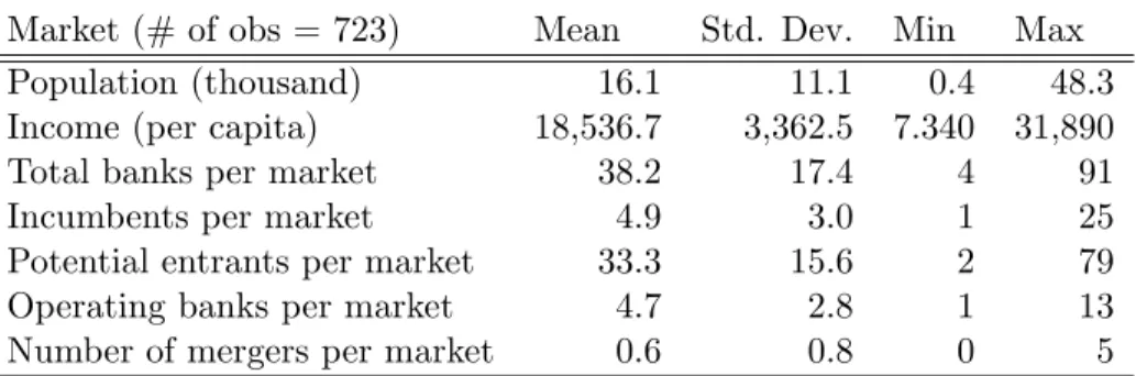
Market (# of obs = 723) Mean Std. Dev. Min Max Population (thousand) 16.1 11.1 0.4 48.3 Income (per capita) 18,536.7 3,362.5 7.340 31,890 Total banks per market 38.2 17.4 4 91 Incumbents per market 4.9 3.0 1 25 Potential entrants per market 33.3 15.6 2 79 Operating banks per market 4.7 2.8 1 13 Number of mergers per market 0.6 0.8 0 5
Table 1: Descriptive Statistics — Market Level
keeps track of the banks’ mergers and acquisitions. Data on merger contracts are obtained from the data set of SNL Financial, which reports deal values for each merger.26
Markets in the banking industry are known to be local in nature.27 Existing works as
well as antitrust analysis use geographic area as the de…nition of a market for the banking industry. Following Cohen and Mazzeo (2007) we focus our attention on rural markets, and we use a county as a market. This is because the typical market de…nition for urban areas (such as the Metropolitan Statistical Area) is likely to include submarkets within it. For this reason we exclude counties with a population greater than 50,000 from our data.28 In such markets, consumers are also very less likely to use banks in other markets.
As discussed in the model section, we classify banks into incumbents and potential entrants in each market. We de…ne banks that have operated in the market as of July 1, 1997 as incumbents. Regarding potential entrants, banks that have operated in a contiguous market during the data period are de…ned as potential entrants. There is a small number of banks that have entered though they are not identi…ed as potential entrants according to this de…nition. Hence, we added these banks to the set of potential entrants as well, which also includes a small number of newly established banks that account for 0.1% of the potential entrants. We identify …rm entry if the …rm exists at the end of our sample period. Table 1 reports the summary statistics of the market-level information. On average, there are 4.9 incumbent banks and 33.3 potential entrants in a market. There is substantial variation across markets for the number of incumbents and potential entrants. Among those …rms, the number of operating banks is 4.7 on average. The average number of mergers per
2 6Merger data of SNL Financial do not necessarily have the same bank names as in FDIC data for the buyer and target banks. About a third of the mergers are matched by the FDIC certi…cation number for both buyer and target banks. Another one third of the mergers are matched by the FDIC certi…cation number of one side, and the holding company name and the FDIC holding company number. For the rest of the mergers, we matched manually using bank and holding company information from both data sets, and other sources such as regulatory …lings. If a merger was still unmatched, we interpolated the transfer using buyer and target characteristics.
2 7See, e.g., Ru¤er and Holcomb (2001), Ishii (2005), and Cohen and Mazzeo (2007).
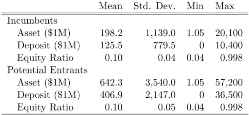
Mean Std. Dev. Min Max Incumbents
Asset ($1M) 198.2 1,139.0 1.05 20,100 Deposit ($1M) 125.5 779.5 0 10,400 Equity Ratio 0.10 0.04 0.04 0.998 Potential Entrants
Asset ($1M) 642.3 3,540.0 1.05 57,200 Deposit ($1M) 406.9 2,147.0 0 36,500 Equity Ratio 0.10 0.05 0.04 0.998
Table 2: Descriptive Statistics — Bank Characteristics.
market is 0.7.29
One of the assumptions of our empirical analysis is that the entry and merger decisions are independent across markets. Regarding this point, more than 80% of the incumbents were present only in one market, and more than 95% of the incumbents were present in less than three markets. Regarding actual entry, both the incumbents and potential entrants enter only one market in about 80% of the cases and less than three markets in more than 95% of the cases for incumbents and 92% for potential entrants. Conditioning on entry with merger, both types of banks enter less than three markets in 92% of the cases. Thus, in the vast majority of our data, banks do not overlap across markets, and we treat markets independently. The fact that our data is mostly from small regional banks in small regional markets helps us on the independence assumption.
Table 2 reports the summary statistics of the bank-level information. The incumbents’ mean size of assets is much smaller than that of potential entrants at $198.2 million. This may re‡ect the fact that we de…ne potential entrants as banks in contiguous markets, which tend to be larger than the market we consider. Descriptive statistics on the equity ratio are roughly the same for incumbents and potential entrants with a mean of 10%.
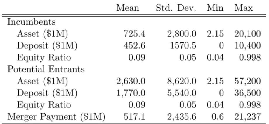
Table 3 provides the descriptive statistics of the same variables included in Table 2 for incumbent and potential-entrant banks that enter the market with a merger, respectively. Table 3 also reports the merger payment from buyer to target banks, which includes not only cash payment but also payment by share. As we saw in Table 2, the mean size of assets and deposits for incumbents is much smaller than that of potential entrants at $2,630 million and $1,770 million, respectively, while the equity ratio is almost the same. Comparing Tables 2 and 3, the average size of the assets and deposits are much larger for banks that
Mean Std. Dev. Min Max Incumbents
Asset ($1M) 725.4 2,800.0 2.15 20,100 Deposit ($1M) 452.6 1570.5 0 10,400 Equity Ratio 0.09 0.05 0.04 0.998 Potential Entrants
Asset ($1M) 2,630.0 8,620.0 2.15 57,200 Deposit ($1M) 1,770.0 5,540.0 0 36,500 Equity Ratio 0.09 0.05 0.04 0.998 Merger Payment ($1M) 517.1 2,435.6 0.6 21,237
Table 3: Descriptive Statistics — Bank Characteristics of the Merged Banks
enter the market with a merger, and also the standard deviations are much larger for those banks.
4
Identi…cation and Estimation
In this section, we propose an estimation strategy for two-sided matching models based on moment inequalities and equalities. One of the major issues of estimating two-sided matching models is addressing the multiplicity of stable matchings. Our estimation strategy uses moment inequalities to deal with the issue of multiple equilibria similar to recent studies estimating noncooperative games by a set estimator (Ciliberto and Tamer, 2009, Ho, 2009, Kawai and Watanabe, forthcoming). We do so by exploiting the lattice structure of the set of equilibria (orN-stable outcome, to be more precise). Before presenting our identi…cation and estimation strategies, let us …rst describe the speci…cation of the payo¤ function.
4.1 Speci…cation
First, we provide a speci…cation regarding the …rm payo¤s. In our environment pro…ts depend on the outcome of the matching game as well as the …rm and the market character-istics. As discussed in the model section, we follow Bresnahan and Reiss (1991) and assume that the number of operating …rms, N, negatively a¤ects the pro…t of the …rm (note that
N depends on entry and merger decisions jointly). The speci…c form of the pro…t function we consider for incumbenti(for entry without merger and no entry) is
where is the degree of the negative externalities due to competition, and i(k;Ni)
i(k;Ni(k))with slight abuse of notation. Market characteristics, which include population
and average income, are denoted by z and the e¤ect of market characteristics on pro…t is captured by 0. The e¤ect of …rmi’s characteristics,xi, in the case of entry without merger
is denoted by 1. Regarding …rm-speci…c characteristics, we consider each bank’s equity ratio and asset size. The next term, 2I, is a constant term for incumbents entering without merger. The last term, m, denotes market-level pro…t shock, which is an i.i.d. draw from a normal distribution, N(0;1). This is for a normalization. If the …rm does not enter the market, the pro…t is zero. Similarly, we write the pro…t function for entrant e (for entry without merger and no entry) as
e(e;Ne) = Ne+z 0+xe 1E+ 2E+ m, e(o;Ne) = 0,
wherexe denotes …rme’s characteristics, and 2E is a constant term for potential entrants,
which we allow to di¤er from 2I for incumbents. As in the case of incumbents, …rm e’s characteristics (xe) include the equity ratio and the asset size. The di¤erence between 2E
and 2I captures the di¤erence of entry costs across potential entrants and incumbents, if they enter the market without merger.
Next, in order to write the pro…t for the case of entry with merger, we start with the pro…t of the merged entity. The pro…t after merger between …rms e and i given the (dis)synergy functionf and the estimation by …rm j2 fe; ig, (kei;Nj), is written as
(kei;Nj) = Nj+z 0+f(xi; xe; xie) + m,
f(xi; xe; xie) = 2M +xi 3+xe 4+xixe 5+xie 6,
where the synergy or dissynergy of a match is represented by a synergy functionf(xi; xe; xie),
which depends on …rm i’s characteristics (xi), …rm e’s characteristics (xe), and
match-speci…c characteristics (xie). For match speci…c characteristics, we use the distance between
the headquarters of two banks and the indicator variable for the same bank holding com-pany. 2M is a constant term for (dis)synergy, 3 and 4 are the e¤ects of the incumbent’s and potential entrant’s characteristics on (dis)synergy of the merger, respectively, and 5 captures the e¤ect of the interaction terms of both …rms’ characteristics on (dis)synergy.
6 measures how the match-speci…c characteristics such as the distance between
headquar-ters a¤ect the (dis)synergies.30 Note that we do not consider (dis)synergies across markets
3 0Note that the match speci…c characteristics,x
although such factors may be present in some industries. This is because vast majority of banks are present only in one market in our data as described in the data section.
Because the terms of merger contracts take cash and stock as medium of payment, we consider the space of the term of tradePasP =T R, whereT =ft; :::;0; :::; tgcorresponds to a …nite set of cash transfers, andR=f0; :::;1gcorresponds to a …nite set of stock shares betweeneand iafter merger. Now we can write the pro…t function for the case of mergers with contractkei for …rmseand ias
e(kei;Ne) = rei (kei;Ne) tei; i(kei;Ni) = (1 rei) (kei;Ni) +tei,
where tei 2T denotes a cash transfer from eto iand rei 2R denotes a payment in stock
shares of the merged entity from eto i. Note that both rei and tei are observable for the
realized merger contracts as data.
Finally, we specify the payo¤ of each …rm considering both pro…t and other factors. As discussed in the model section, we allow idiosyncratic factors to a¤ect entry and merger decisions because these factors such as the degree of shareholder control, CEOs’ tastes and abilities may play an important role as illustrated in Jensen and Meckling (1976), Malmendier and Tate (2008) and Goldfarb and Xiao (2011).
We consider such idiosyncratic shock"iefor …rmimerging with …rme, and"iifor …rmi
entering without merger. These idiosyncratic shocks are unobservable to the econometrician though they are observable to the …rms. Similarly we have "ei for …rm emerging with …rm
, and "ee for …rm e entering without merger. These shocks are i.i.d. draws from the
standard normal distribution.31 Furthermore, the relative importance of shocks"
ie and"ei
to the monetary pro…t are allowed to be di¤erent across banks. Speci…cally, we capture the relative importance of the idiosyncratic shocks to j by I for incumbents and by E for
potential entrants. We thus write the payo¤ of incumbent ias
i(kei;Ni) =
1
I i
(kei;Ni) +"ie;
i(i;Ni) =
1
I i
(i;Ni) +"ii;
i(o;Ni) = 0;
and the payo¤ of potential entranteas
e(kei;Ne) =
1
E e
(kei;Ne) +"ei;
e(e;Ne) =
1
E e
(e;Ne) +"ee;
e(o;Ne) = 0:
For notational convenience, we de…ne ( ; 00; 01; 2I; 2E; 2M; 03; 04; 05; 06; I; E),
and the space of as .
4.2 Identi…cation
4.2.1 Identi…ed Set
Our identi…cation is based on the restrictions provided by the equalities (1) and (2) in Corollary 1 and the inequalities (3) and (4) in Corollary 2. In Corollary 2 we show that the payo¤s in the two extremum equilibria (orN-stable outcomes to be more precise),K E and
KI , are the upper and lower bounds of any equilibrium payo¤. Hence they constitute the bounds of the payo¤s corresponding to the observed data. Furthermore, Corollary 1 shows that, in anyN-stable outcome, the number of operating …rms is the same. Also, the payo¤s of …rms that do not merge are the same in any N-stable outcome. These results lead us to construct moment equalities regarding the number of operating …rms and the payo¤s of non-merging …rms. Hence the observed data should match the number of operating …rms and the payo¤s of non-merging …rms in K E and KI .
Let us …rst revisit the result of Corollary 2 (more speci…cally, equations (3) and (4)): the two extremum N-stable outcomes provide the highest payo¤ to one side of the banks and the lowest payo¤ to the other side, i.e., (suppressing the dependence on N for notational convenience) for any N-stable outcomeK ,
e(K
E
; ) e(K ; ) e(K
I
; ),8e2 E,
i(K
I
; ) i(K ; ) i(K
E
; ),8i2 I.
In other words, given ,e’s payo¤ in anyN-stable outcome is bounded above by the payo¤ in theE-optimalN-stable outcome, e(K
E
; ), and bounded below by the payo¤ in theI -optimalN-stable outcome, i(K
I
; ). Similarly the payo¤s for all incumbents are bounded above and below by i(K
I
; )and i(K
E
; ), respectively. Observe that we can compute these bounds given (and shocks) using the algorithm shown in Section 2.3.
We can also compute the payo¤s for each …rmjcorresponding to the data, j(K DAT A
as K DAT A. Though we cannot know which equilibrium the data-generating process cor-responds to, the payo¤ corresponding to the equilibrium in the data must still be bounded by j(K
I
; ) and j(K
E
; ) for all j. Hence, we can consider the following types of inequalities:
Eh e(K
E
; ) e(K DAT A
; )jXi 0, (5)
Eh i(K
I
; ) i(K DAT A
; )jXi 0, (6)
Eh e(K DAT A
; ) e(K
I
; )jXi 0, (7)
Eh i(K DAT A
; ) i(K
E
; )jXi 0, (8)
where X = f(xi1; :::; xiNI);(xe1; :::; xeNE); zg denotes …rm characteristics of all …rms in a market and market characteristics. Note that these inequalities are at the level of indi-vidual …rms. However, our unit of observation is a market, and identity and number of incumbents and potential entrants di¤er across markets. Thus, we use moments based on these inequalities at market level in our estimatio, which we describe in Appendix B (we construct 44 moment inequalities.).
Next, we discuss moment equalities resulting from Corollary 1 (more speci…cally, equa-tions (1) and (2)). Part (iii) of Corollary 1 shows that the number of operating …rms and the number of mergers are identical in any N-stable outcome (equation (2)). Though the econometrician cannot know which equilibrium the data-generating process corresponds to, the number of operating …rms and the number of mergers are the same in any equilibrium (or in any N-stable outcome). Thus, the observed data on the numbers of operating …rms and mergers equal those in the two extremum N-stable outcomes, K E and KI , and we can write the following equalities:
E NmergeDAT AjX = Eh (K E; NDAT A; )jXi=Eh (K I; NDAT A; )jXi;
E NDAT AjX = Eh (K E; NDAT A; )jXi=Eh (K I; NDAT A; )jXi; (9) whereNDAT A
merge and NDAT A are the numbers of mergers and operating …rms in the observed
data. Regarding Part (ii) of Corollary 1, we have equation (1) which states that unmatched (non-merging) …rms earn exactly the same payo¤ in anyN-stable outcome, i.e., for any j
choosing either fjgorfog, we have
Eh j(K DAT A
; )jXi=Eh j(K E; )jX
i
=Eh j(K I; )jX
i
. (10)
de-scribe the moments we use in our estimation based on these equalities in Appendix B (we construct 14 moment equalities.).
Finally, we de…ne the identi…ed set id using both moment inequalities and equalities
as id=f 2 :inequalities (5)–(8) and equalities (9) and (10) are satis…ed at g.
4.2.2 Exclusion Restrictions
Our identi…cation depends on two types of exclusion restrictions: the exclusion restriction employed in the regular entry model and the exclusion restriction for the synergy function.32 We need these two types of exclusion restrictions becausexiandxea¤ect not only the payo¤
of entering without merger but also the payo¤ of entering with merger.
The …rst type of exclusion restriction we use is the one adopted in the literature on estimating entry models. As in Berry (1992) and Tamer (2003), we need a variable that a¤ects a …rm’s pro…t but does not enter the other …rms’ pro…t functions. In our model, the asset size of a bank, xasset
j , serves as an exclusion restriction of this type: In the banking
literature, demand is typically modeled as a function of geographic proximity to the banking facility and interest rate (see, e.g., Ishii, 2005), while the asset size is an important factor on the cost side (see, e.g., McAllister and McManus, 1993).
The second type of exclusion restriction we use concerns the identi…cation of the synergy function. To identify synergy function f, the …rst type of exclusion restriction does not su¢ce if all exogenous variables inf are also included in j(j; N) (payo¤ for entry without
merger). Thus, we require a match-speci…c variable that enters the synergy function, but a¤ects neither the (dis)synergy of any other combination of …rms nor the payo¤s of the two …rms entering without merger.
In our speci…cation, we use the distance between the headquarters of the incumbent and the potential entrant, which is the …rst element of xie, x(1)ie . This variable a¤ects the
post-merger synergy for various reasons, such as communication between the workers of the target and acquiring banks, while it is unlikely to a¤ect the payo¤ of entry without merger and mergers of any other bank pairs.
Our identi…cation argument proceeds in two steps using the two types of exclusion restrictions in each step. First, we use the second type of exclusion restriction to identify all the parameters that are not included in the synergy function. The assumption we need is that f(xi; xe; xie) ! 1 as x(1)ie ! 1, i.e., the dissynergy goes to in…nity as the
distance becomes in…nity. This implies that asx(1)ie ! 1 we obtain e(kei; N)! 1 and