本文 総合研究大学院大学学術情報リポジトリ 乙182 本文

! " # $! !

% $ &#' ・・・・・・・・・・・・・・・・・

( ) ・・・・・・・・・・・・・・・・・・・・・

! *& % + % !・・・・・

, # % $ &#' ・・・・・・・・・・・・・

- ・・・・・・・・・・・・・・・・・ _.

/ ! ・・・・・・・・・・・・・・・・・・・・・ _.

. - & ・・・・・・・・・・・・・・・・・ ₀

0 1 % ・・・・・・・・・・・・・・・・・ ₂

2 & # ・・・・・・・・・・・・・・・・・・・・ ₂

& % % $ &#' ^{・・・・・・・・・} 3

3 - ・・・・・・・・・・・・・・・・・・・・

・・・・・・・・・

4 ! ・・・・・・・・・・・・・・・・・・

& + & % $ &#' ・・・・ /

5 & % $ &#' ^{・・・・・・・・} /

6 7 # 1 89 ・・・・・・・・・・・・ ₀

4 : 6 ・・・・・・・・・・・・・・・・ ₂

$ & & + + & & && ・・・

6 7 # + + : & 5 && ^・・・

5 46 ( 6 ・・・・・・・・・・・・・・・・

& 1 ・・・・・・・・・・・・・・・・

/ - + % ・・・・・・・・・・・・

. % *& ! ・・・・・・・・・・・・ _.

/ ; & 46 ・・・・・・・・・・・・・・・・・・ 0

/ ; & 46 % ! ・・・・・・・・・・・・・・・・ 2

/ < ! ; ・・・・・・・・・・・・

. 6 - & 6 & ^{・・・・・・・・・} /

. / % & 5 + ^{・・・・・・・・・} /2

. . $ & 6 & ・・・・・・・・・・・・・ _.

. 0 - & ( !+ ! ・・・・・・・・・・・・・ _.

. 2 - + & ^{・・・・・・・・・} ./

0 5 + % $ &#' ・・・・・ .2

0 6 ・・・・・・・・・・・・・・・・・ _.2

0 % ; % % % ・・・・・・・・・・・・ _.

0 & & ! - & ( !+ ! ・・・・・・・ 0

0 / = 1 ・・・・・・・・・・・・・・・・・ _0/

2 ( !+ ! & ! - & 6 & ・・・・・・・ 0.

2 & ! % % ・・・・・・・・・・・ _0.

2 5* ! & ・・・・・・・・・・・・・・・・ 0.

2 ; ・・・・・・・・・・・・・・・・・・ ₂

2 / 1 & ・・・・・・・・・・・・・・・・・・ ₂

+ % ! ! 66 % ! ・・・・・・・・・・・・ 2.

; & 46 % ! ・・・・・・・・・・・・・・・・ 2.

66 ・・・・・・・・・・・・・・・・・・・・ _2.

6 7 # & >-(?9 66 ^{・・・・・・・・} 22

/ ( !+ ! ! & ! !# % ^・・ 2

. - & % ・・・・・・・・・・・・・ ₂₃

0 ;1 - 66 % ! ^{・・・・・・・・・}

3 & & 66 % ・・・・・・・・・・・・

3 5 & % % ^{・・・・・・・・・}

3 + - ・・・・・・・・・・・・・・・・・

3 $ & % % ・・・・・・・・・・・・・

3 / ; % 66 ! ^{・・・・・・・・・} .

・・・・・・・・・・・・・・・・・・・・・

! ・・・・・・・・・・・・・・・・・・・・・

・・・ 3

4 !

・・・・・・・・・・・・・・・・・・・・・・

# + % ! ・・

・・・・・・・・・・

( ) ! + % ! ・・・・・・・・・・

% & % ! & + % ! ・・・・・

4% & % + % ! ・・・・・・ 3

& + !

・・・・・・ 3/

4 + ! ・・・・・・ 3/

4 & ・・・・・・ 3.

& ・・・・・・ 33

/ & & ^・・・・・・・・・・

. @ % % + ^{・・・・・・・・}・・・・・・

/ 1 % & @ & ! ; & #

^{・・・・・・・・}・・・・・・

. %% # ・・・・・・・

・・・・・・・・・・・・・・ /

0 - ・・・・・・・

・・・・・・・・・・・・・・ /

!"

^{・・・・・・・・・・ .}

/ 4 !

・・・・・・・・・・・・・・・・・・・・・・ .

/ A@ % & # %

・・・・・・・・・・・・・・・・・・ .

/ 5 + # % ・・・・・・・・・・・・・・・・・・ .

/ & & + # % ・・・・・・・・・・・・・・・・ 2

/ A@ & + # % ・・・・・・・・・・・・・

/ / 1 & ・・・・・・・・・・・・・・

/ . 4% & % & ・・・・・・・・

/ 0 % & 7 # ! % ^{・・・・・・・・}

/ 2 " % ・・・・・・・・・・・・・・

/ 1 1 & 6 & ^・・・ .

/ 3 ! + % 1 ! & ! ^・・・ .

/ ; 4 & * % ^{・・・・・・}

/ # ! 1 ;;1 > 1/ 09

^{・・・・・・}

/ 5 & ; & ; + 1 1 & ^{・・・・・}

/ 141 6 & ・・・・・・・・・・・・・・・・・・

/ ; * $ % >;$9 % ! 64- 6 & ^・・・・

/ / $ % ; % ・・・・・・・・・ /

/ . 1 64- & ・・・・・・・・・・・・・・ /

/ / @ % & # %

・・・・・・・・・・

/ . %% #

・・・・・・・・・・・・・・・・・・・・・・ 3

/ 0 -

・・・・・・・・・・・・・・・・・・・・・・ 3

/ 2 $ ! @ : #

・・・・・・・・・・・・・・ 3

# $

・・・・・・・・・・・・・・

. / A % ) : & ^{・・・・・・・・・・} /

. - &

・・・・・・・・・・・・・・・・・・・・・・・

. % & & ・・・・・・・・・・・・・・・・・・

. - & ) & & ! ^{・・・・・・・・・・} /

. - & * ! -(? ^{・・・・・・・・・・} /

. / ;

・・・・・・・・・・・・・・・・・・・・・・ .

. / ) & & - ! ・・・・・・・・・・・・・ _/.

. / ( ! & * !+ ! ^{・・・・・・} /.

. / & ! % @ % % + ^{・・・・・} /.

. . %% # ・・・・・・・・・・・・・・・・・・・ /0

. 0 - ・・・・・・・・・・・・・・・・・・・ /0

% &

・・・・・・・・・・・・・・ /2

0 4 !

・・・・・・・・・・・・・・・・・・ /2

0 - 7 ! ! +

・・・・・・・・・・ /2

0 5 % ・・・・・・・・・・・・・・・・・・ /2

0 5 % % & % ・・・・・・ /

0 - 7 ! % ・・・・・・ .

0 / - & * + 46 * !+ ! ! % & 7 # .

0 . 4% & % % & @ & ・・・・・・ .

0 ; & # + % !

・・・・・・・・・・・・・・ ./

0 / 6 & % ! # ' 7 #

・・ .0

0 / 5 + & # ! # ' # % ・・ .0

0 / ! & ^・・・・・・ .0

0 / # ' * + % ! % & ^・・ .

0 . - 46 &

・・・・・・・・・・・・・・・・・・ 0

0 0 + ! ! 1 = %

・・・・・・ 0

0 0 & ( ) ! ・・・・・・・・・・・・・・ 0

0 0 % & $ &# ・・・・・・・・・・・・・・ 0/

0 0 % & $ &# + ! ・・・・・・ 02

0 2 - + &

・・・・・・・・・・ 03

0 4 &

・・・・・・・・・・・・・・ 2

0 % $ &#' ・・・・・・・・・・・ 2

0 & & && ・・・・・・・・・・ 2

0 46 & ・・・・・・・・・・・・・・ 2/

0 3 A@ % & %

・・・・・・・・・・・・・・ 22

0 3 -(? ,' ・・・・・・・・・・・・・・・・・・ 22

0 3 -(? ,' ・・・・・・・・・・・・・・・・・・ 2

0 3 -(? ),' ・・・・・・・・・・・・・・・・・・ 23

0 3 / -(? ),' ・・・・・・・・・・・・・・・・・・

0 B + )

・・・・・・・・・・・・・・

0 1 % % !

・・・・・・・・・・・・・・ .

0 -

・・・・・・・・・・・・・・・・・・ 2

' & &

・・・・・・・・・・・ 3

2 4 !

・・・・・・・・・・・・・・・・・・・ 3

2 4% % - + % !

・・・・・・・ 3

2 5* ?/3

・・・・・・・・・・・・・・・・・・・ 30

2 1 % 66 % ! 5* ?/3

・・・ 30

2 / 5* & C %

・・・・・・

2 . ; 5* 2 2 ! 2 /

・・・・・・

2 0 1 = % # % -A$

・・・・・・ /

2 2 1 % !

・・・・・・・・・・ 0

2 2 @ % % + ・・・・・・・・・・・・・・ 0

2 2 % & ! % ・・・・・・・・・・・・・ 2

2 2 ! - ( !+ ! ! $7 % ^・・・

2 1 &

^・・・・・・・・・・・・・・・・・

2 3 -

^・・・・・・・・・・・・・・・・・

(

^・・・・・・・・・・・・・・・・・

1 &

^・・・・・・・・・・・・・・・・・・・・・

*

・・・・・・・・・ /

- ・・・

・・・・・・・・・・・・・・・・・ .

) * + ,

^{・・・・・・・・・・・・・ 0}

* ,

) : & - ! % & ' ! + -

・・・・・・・・・ /3

( ! -*+ % & ' ! + -

・・・・・・・・・ .

& 6 D .

・・・・・・・・・・・・・ 0.

/ 1 ? ! +

・・・・・・・・・・・・・・・・・ 22

. - & # $ >- ! E + & ' 6 " 09

・・・・・・・・・ .

. * - & # ( >$ & A $ 09

・・・・・・・・・・・・・ .

0 1 % !

・・・・・・・・・・・・・・・・・ 2

/ & % ! @ %

・・・・・・・・・・ /

/ % & ' ! + F) ! $ ! + %

-(? && ! ,' ・・・・ 2

/ $ % ; % ・・・・・・・・・・・ /

/ / 1 16 - & G H0 I > $ 9 ・・・・・・・・ .

/ . 1 6 - & G H0 I >0 $ 9 ・・・・・ .

/ 0 % # @ % & # % ・・・・・・・・

. - & ・・・・・・・・・・・・・・・・・・・

. - & ・・・・・・・・・・・・・・・・・・・ 3

. - & & % &#' > 9 - 0/ ・・・・・ /

. / ) : & - ! % & ' ! + ・・・・・・・・・ /

. . F) ) : & ! ! !( ・・・・・・・・・ /

. 0 ( ! -(? % & ' ! + ・・・・・・・・ /

. 2 F) ! ・・・・・・・・・・・・・ //

0 5 % @ % & # % >; % & @ & 9 ・・・ /

0 5 % @ % & # % > % & @ & ;;19 .

0 A@ % & ! 6 0 ・・・・・・・・・・・・ 03

0 / 1 % % % % % ! ・・・・・・・ .

2 1 ! % ・・・・・・・・・・・・・・・ 3

2 - 4 & % ・・・・・・・・・・・・・・・ 3/

2 ! ! ! 4 & % ・・・・・・・・・・ 03

* -

A@ % & + ・・・・・・・・・・・・

1 % +

* + + % ! ! + % ! ・・ 0

% & ! & # % &#' ・・・・・・・・・・・・・

(& ) ; % 1& + % $ &#' ・・・・・・ .

(& ) ; % 6 7 # 1 ・・・・・・・・・・・・・ 2

6 7 # ! % @ ・・・・・・・・・・・・・・・・ 2

/ 6 7 & ! % @ + + & & ・・・・・・ 3

. % 6 7 # ! % ! % @ + + & & ・・・

0 & 7 # ・・・・・・・・・・・・・・・・・・・

2 - -(? & % 1? & ・・・・・・・・ /

A@ % & + ・・・・・・・・・・・・・ .

3 (& ) ; % + % &#' + ! & 46 ・・・・・・ .

; & ! & 46 ・・・・・・・・・・・・・・・・ 2

< ! ; 6 7 # ; % ・・・・・・・・・

; ' ! 46 & + + & & && > 9 ^{・・・・・・}

< ! ; ! 46 & + ! * ! : 6 > 9 ・・

/ < ! ; ! 46 & -(? 6 & ：

_H

_{> 9} ・・ /

. % A@ ! % &

_H

> 9 ^{・・・・・・・・・} /

0 & 6& + + % &#' + ; & 46 # % ・・ .

2 % & ! (& ) ; % + % $ &#' + ; & 46 0

1 & ! % + % ! ・・・・・・・・・・・ /

3 A@ % & + ・・・・・・・・・・・ /

+ % ! + ・・・・・・・・・・・・・・・ /

% & & A7 > /2 *9

- & ! * * ! &

" #

$ J ),' -(?J ),' J % ) & & J !( F)J .

$%

/

% + &

・・・・・・・・・・・・・・・ .

. ( ( ! & ! % + &

J ),' -*+J ),' + % J %

> 9

% + & ⊿ J . ,'

・・・・・・・・・・・・ ..

>*9

% + & ⊿ J ,'

・・・・・・・・・・・・ ..

> 9

% + & ⊿ J ,'

・・・・・・・・・・・・ .0

>!9 % + & ⊿ J ,'

・・・・・・・・・・・・ .0

0 >( !+ ! & #9 0 !( ! !( * !+ ! .

2 % ! % % % ・・・・・・・・・・・・・・・・ .3

% ;# % & & ・・・・・・・・・・・・・・・ 0

3 A7 & ( !+ ! >A (?9 & & ・・・・・・ 0

- & * + & & ! -(?

> 9 5* ! & & & > F 9 ・・・・・ 0

>*9 & + & & & ! -(? ・・・・・・・・・・・・ 0

= 1 ・・・・・・・・・・・・・・・・・・・・・・ 0/

% + ! * ! & + -(? ,' ・・・・・・ 02

% + ! * ! & + -(? ),' ・・・・・・ 0

/ % + ! * ! & + -(? ),' ・・・・・・ 03

. % + ! * ! & + $ ),' ・・・・・・ 2

0 1 & 6 & ! -(? & ・・・・・・・・・ 2

2 ;# % 6 % ! & ! -(? & ・・・・・・・・・ 2/

A@ % & (& ) ! % 66 % ! ・・・・・・・・・ 2.

3 1 66 ・・・・・・・・・・・・・・・・・・・・・・・ 20

/ A@ % & && : ・・・・・・・・・・・・・・・・ 2

/ ( !+ ! ! & % ! ! 66 % ! ・・ 23

/ - & % 66 % ! ・・・・・・・・・・・・・

/ K ! *# + % ! ・・・・・・・・・・・・

// + $ ・・・・・・・・・・・・・・・・ /

/. - & % *# + % ! ・・・・・・・・・ 0

; % A@ % & # % ・・・・・・・・・・ 3

5 + ; & ; + 1 >;;19 ・・・・・・・・・・ 3

( * ! & + % ! ・・・・・・・・・・・・ 3.

/ ! 1 ! * * ! & ! ・・・ 32

. 6 & -(?J ,' ・・・・・・・・・・・・・・・・ 3

0 6 & > -(?J ,'9 > 9 & ・・・・・ 33

2 % & % ! & ・・・・・・・・・・・・・

6 7 # ! ・・・・・・・・・・・・

3 - % ! 7 # & ・・・・

& 6& + 1 % & @ & ・・・・・・・・・・・・・・・

/ 5 + 5 A@ % & # % ・・・・・・・・・・・・ 0

/ - & & + A@ % & # % ・・・・・・ 0

/ 5 + & 6& + A@ % & # % ・・・・・・ 2

/ / 5 + A@ % & # % ・・・・・・・・・・・・

/ . 4 & + ; " ・・・・・・・・・・・・・・・・ 3

/ 0 4 & *& ) ! % ; " ・・・・・・・・・・・・ 3

/ 2 1 ( ! : % 6 & ・・・・・・・・・・・・・

/ 6 & >!(9 ! % % % & - ・・・・・・

/ 3 % & - % ! ・・・・・・・・・・・・・・・・

$ 3 / 4 // 5

/ .

F /

F ^{= ⋅ = ⋅}

σ

=

_{・ ・ ・} ・・・・・・・・・・・・ 1

$ & 3 / 4 // 5

F 0

/

F ^{= ⋅ = ⋅}

σ

=

・・・・・・・・・・・・ 1

/ ; 4 & @ %

・・・・・・・・・・・・

3

/ ; + 1 1 &

・・・・・・・・・・・・・・・・

/ 141 ; % 6 &

・・・・・・・・・・・・・・・・・・・

/ / 141 6 & 6 7 # - J/ J -J2 ! J F

・・・・・

/ . 6 7 # - 141 6 & ! ' 7 #

・・・・・

/ 0 4&& ! & % 64- &

・・・・・・・・・・・・

/ 2 1 64- & ;$ % !

・・・・・・・・・・・・

/ 6 G H0 I > $ 9

・・・・・・・・・・・・・・・

0

/ 3 6 G H0 I >0 $ 9

・・・・・・・・・・・・・・・

0

/ 6 7 # 164- + 6 -

・・・・・・・・・・・・

2

. / ) : & - ! % & ' ! +

・・・・・・・

/

. . ( ! -(? F)

・・・・・・・・・・・・・・・

//

0 4 & 7 # ! % * + % & % /3

0 - & * + 46 & ! % & 7 #

・・・・・・・・

.

0 1 % & @ & ;$ 64- & ;;1 1/ 0

・・・・・・・・・

.

0 / & ; & # 1

・・・・・・・・・・・・・・・・

..

0 . $ & $ & ; & # - 0/

・・・・・・・・・

..

0 0 1 6 & ! : #

・・・・・・・・・・・・・・・

.0

0 2 : # ! 6 &

・・・・・・・・・・・・・・・

.2

0 # ' *

・・・・・・・・・・・・・・・

.3

0 3 & & + % &#' *# 66 % !

・・・・・・・

0

0 % 66 % ! + 46 7 #

・・・・・

0

0 1 1 = %

・・・・・・・・・・・・・・・

0

0 > 9 % *# + ! > !(9

6 & > 9 $ ! ( ( ! & >4 ! <9

・・・・

0/

0 >*9 4 ! < % > 9

・・・・・・・・・・・・

0.

0 > 9 % > 9 ⁻ > F 9 >*9

・・・・

0.

0 >!9 ; >*9

・・・・・・・・・・・・・・

00

0 > 9 ! ! >*9

・・・・・・・・・・・・

00

0 > 9 % *# + ! > !(9

6 & > 9 ! ( ( ! & >4 ! <9

・・・・・

02

0 >*9 % > 9

・・・・・・・・・

0

0 > 9 ! ! >*9

・・・・・・・・・

0

0 / > 9 % + &

⊿

J . ,' + % %

・・・・

2

0 / >*9 % + &

⊿

J ,' + % %

・・・・

2

0 / > 9 % + &

⊿

J . ,' + % %

・・・・

2

0 / >!9 % + &

⊿

J ,' + % %

・・・

2

0 . ! & % &#'

・・・・・・・・・・・・

2

0 0 + % $ &#'

・・・・・・・・・・・

2

0 2 ; % ! ! % @ % & # %

・・・・・・・・・

2/

0 5* ! % + !

・・・・・・・・・

2.

0 3 46 & ! %

・・・・・・・・・・・・・・・・

20

0 % + -(? ,'

・・・・・・・・・・・・・・・・

22

0 % + -(? ,' ! ),' $ ),'

・・・・・

2

0 > 9 % + -(? ),' $ / ,'

・・・・・・・・・

23

0 >*9 % + -(? ),' $ / ),'

・・・・・・・・・

0 > 9 % + -(? ),' $ ,'

・・・・・・・・・

0 >*9 % + -(? ),' $ ,'

・・・・・・・・・

0 / > 9 % % ! *# - 0/

・・・・・・・・・・・・

0 / >*9 % % ! *# + % !

・・・・・・・・・

0 / > 9 5 & # % > 9 ! >*9

・・・・・・・・・・・・

0 . % F6 7 # ; % 46 & ! & &

・・・・・

/

2 # % % -

・・・・・・・・・・・・・・・

3

2 > 9 ! % + % &#' + $B 3

2 >*9 % % ! + $B

・・・・・・・・・・・・・・・

3

2 > 9 % % ! + % ! + $B 2

・・

3

2 >*9 % % ! + % ! + $B 2

・・・

3

2 / - 4 & %

・・・・・・・・・・・・・・・・・・・

3/

2 . ! ! ! 4 & %

・・・・・・・・・・・・

3.

2 0 % ,#! ?/3

・・・・・・・・・・・・

30

2 2 > 9 % % ! + % !

・・・・・・・・・

32

2 2 >*9 % % + / &

・・・・・・・・・・・・

3

2 2 > 9 % % ! + 3 / &

・・・・・・・・・・・・

33

2 - $ % &

・・・・・・・・・・・・

2 3 & ! *# % & % 3 02 ,'

・・・・・・・・・

2 % & + 6 2 3 % *# + % !

・・・・・

2 $ % & 7 %

& & ! * !+ !

・・・・・

/

2 ; % 564$ -A$ 1 %

・・・・・・・・・

.

2 5 $? % 564$ -A$ 1 %

・・・・

.

2 / $! 1 1 ! % 1 ! 0

0 0

% 6 7 # ; % ! %

! ( !+ ! + !

・・・・・・・・

2 + + # + ! * !

・・・・・・・・・・・・

& .

4 @ %# # ) + ) ! &

% ! ! ; L ! " #

$! ! ! 4 ) +& ! + % !

C 1 ) ! % % + %% ! ! % &

& * + % ! = % ! + ;

4 &! ! 7 & # 4 ) 6 L + + ! ! &

+ 4 + ! ! ! > /9 $ : * # " # ! %

! % & 6 % ! % 4 7 ! 6 L * % %*

L ! %% 4 ) % 7 4 ) ; 4 ; , , ! !

; * ! 4 & ) , ! L % M #

% %* ' + BA:$ 5* # $5K 4 + &! & ) ) ; 6 L + !

; ? L % % C %

4 ) ; % &# 4 &!

+ % % 4 & ) 5 ! + ! * %# &

! %

4 &! ) && & C ? 1 ! % , %

% ! , ) % + ) + % ! % % %

# % G$& 1 I 4 + ! ! *# C ? 1 ! %# &

$ ) ! ) @ 1 # ! & %

&#' ! &# + % !

!"

# # $

% % #

& # ' (

)

%

$

* + % ,*+- .

.

#

#

/ 0/10//20/30

- , - %

# , - + ( % #

, - 45 "'5 '5 " 1 1"

1

# 6 .+

572899 # 5 7 ' .

( #

/80

++ ++

, "'5 - :

# # , "'5

2"'5 - . #

/!0 . ++ %

; % % )6<= %

; % % #

% > #

; % %

# ++

#

&

# # 1 9

) # * + %

,*+- : + .

" 1

≥ , -

" ^{1?2 ( %}

# # .

, + 1 9-

(

- * ( @ ) ( % , -

1- A @ ) '

2- + % @ ) %

& # 1 )

( .

" : ( _" $% , -

" : / 0 /10/20/30

B ( + % + 1"'5

'5 # !"

" !" 1"

$% , - & #

&

# B

$% , -

!" # $

C1"'5 C '5

# @ !" , -

@ " , -

%

# 5 7 ' = , - !" /D0

E D" #

=* . D3

4 $ , ' ( . - # ' / 0 F4 )

) G . # ' 4 $

. D9 = 5798!9)

5798!9)

. 9" , )6H); $ ' ( . -

3

. ++ # ++

% ""'5 #

+ 9"

5798!" , # 57 = - *21!8

, # )6H); $ = - 2""5

""5 ++ #

!9"""

. 9" 57 = 572899 /90 '

. A .

:

572899 # # *+

" #

4

. "J ' ( . F* )

G # ++

. 1""" ) = 7 ) .

) *:& #

) # #

# # '

) #

7 ) / 0 . '

*:& ++

++

*+

#

& '

& ++ )

#

' #

++ ++

7 # +

++ #

# #

++

( )

&

& (

& ++

.

&

.+ , 1 8-

1 &

.+ >

2 &

#

3 & (

(

*+ &

,6 7- .+

, 3 1- # ' '

!

! #

# = K . = !

D #

* ' #

σ -

<

,

χ

σ

≤ ×

! " #

$ "

% &' " $ &' (

1

< 1 =

^σ

= × )

$ *

# ! # +

# " "

+

- ,

"

4 @ _{σ =} ^×

- ,

" σ

"

=

""

=

=

4 ：

1

σ =

σ ₅

, - +

. = 1

.+ # #

) # # ++

. = 2 #

& ( (

. = 3 (

2"

. = 8

. = !

. = D )

B ;*

) # #

( # ++

) ;*

= 9

. /

+ "

+ "

+ "

+ "

-

, ! "

-

L , ^{$ " , -}

$ , " * - " . " ( -.&( -

, $ /

-

,

ω

^{$ * /}

! ! 0

9

-

,

! "

$ "

. +* ) )

,

L ^$

-

,

ω

3

5 5

" ^-

! '&#

&' 6 % . +*

/ '

/ '

/ '

/ '

ω

# *

ω

^{# * "}

, -

ω

# * ! "

, -

ω

# * " , -

"

ω

# 7 *

ω

^{# * " "} , -

σ , 8%&

= 1

σ

σ

( 2 9

⊿ *

- -

- -

-.&( - " "

-$$ -

(:$ ( 0: $

($, ( 0: $ ,

! ! *

! 43 !

13 1

#4 # ;

- %

# #4

#4 $ ! 43 *

# < #

,3-6 * = * "

, ,3-6

, , $

6 >

6 >

6 >

6 >

,?> $ % # 0, % !

#) ; > $ % -.@-6$+,$ (

3,-> $ % -" $ " (

A

A A

A $ $ $ $ $ $ $ $ , , , , - - - - % % % %

- 9 % < " ) $

% "

(((( **** (((( *

,,,, ,3-6,3-6,3-6,3-6 * "

,,

,, > < ,,,, "

> B

< , ,$-#$ ,$$ ! * *

B , ,$C3 ,$3 ! * * "

#### 1111 #1#1#1#1 ! 4

1 = ! "

DEE 4&EE 4&EE 4&<EE 4&

2 '2 '2 '2 ' 2F2F2F2F 2F#2F# !2F#2F# ' *

% @@@@ 4444 @4@4@4@4 !

"

" ) , %

" ) , %

" ) , %

" ) , %

< ^B

0 '

/ 0 4 $ F ) ) G ) 5 # B D3

/10 4 ; F 7 ) G ¹7) M 2 ; 3 6 1"""

D 13

/20 I 6 ' F* G * .

H 39 ; ; DD 3 3 3

/30 * ) & F ; ' G 2 7 5 .

/80 N = = F) " 5 8" 45 ) 6 .+ G

5 7 ' M M

/!0 F ) *O + E G H " "" 4 1""! * O I #5 O = NI

/D 0 5 7 * = ; @

F ) ) G

@<< < #L < L#L L"3

/90 N = = F) " 5 8" 45 ) 6 .+ G

5 7 ' M M

/ 06 # F G $6; <12<1"""

Chapter 2

Review of Sweep-Signal Method

2.1 Introduction

The theoretical backgrounds of the sweep spectrum analyzer are well summarized in the references [1][2][3]. In this chapter, we present detailed analysis of the method on the signal processing.

Section 2.2 shows the outline of the sweep spectrum analyzer. Section 2.3 describes the principal theory of the sweep method. Section 2.4 describes the digital IF method as an improvement of the sweep method. Section 2.5 shows the mechanism of the sweep method as the digital signal processing. Section 2.6 describes a few important characteristics of the sweep method. Section 2.7 investigates the property of the resolution filter in case of measuring the FM modulated signal. Section 2.8 describes the some characteristics of the FFT method. And section 2.9 concludes this section.

The description of this chapter introduces the fundamental of the new method, which is described in chapter 3.

- 13 -

2.2 Principle of Sweep-Signal Spectrum Analyzers

This section describes the structure and the properties of the conventional sweep spectrum analyzer. Section 2.2.1 describes the outline, section 2.2.2 will describe about a frequency down converter, and section 2.2.3 describe the function of the LPF.

2.2.1 Outline of Spectrum Analyzers

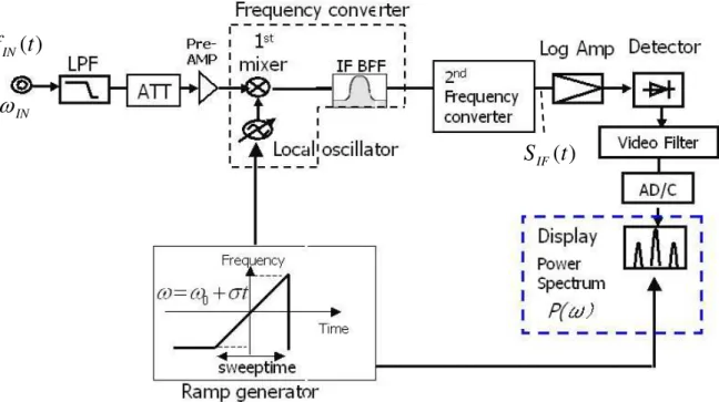
A simplified block diagram of a traditional sweep spectrum analyzer is shown in Figure 2.1. This kind of analyzers consists of many components as follows [1].

・LPF

・ATT & Pre-AMP

・Frequency Converters

・Log AMP

・Detector

・Video Filter

・AD/C

・‘LPF’ (low pass filter) prevents the mixer from receiving higher frequency signal than the system cannot process. A function of the LPF is described in section 2.2.3.

・’ATT’ (attenuator) is used to degrease the power of the input signal, in the case that the power of the input signal is too large. And ATT is used to reduce the noise power of the input.

・Usually sweep spectrum analyzers have multiple ‘Frequency converters’. They consist of a mixer, a local oscillator and a band pass filter and output of IF (Intermediate Frequency) signal

‘S_IF

(t )

’. It is described in section 2.2.2.

・The ‘Log Amp’ converts the amplitude of the S_IF

(t )

logarithmically.

・The ‘Detector’ detects the output of the Log Amp with AM detection.

・The ‘Video Filter’ limits the bandwidth of the detected signal and outputs the

envelope

of the . In the classic sweep spectrum analyzer with analog displays, this signal was used to drive the vertical deflection plate of the CRT directly. Hence the signal is called ‘Video signal’. Most spectrum analyzers since 1980s digitizes the Video signal with the ‘AD/C’, AD converter, and the spectrum is displayed by a digitized display.

) (t S_IF

・The digitized data is put into memory of the ‘Display system’, which is controlled by a microcomputer or other control devices. The Display shows the Video signal as the ‘Power Spectrum: P(ω)’.

)

S

_IF

(t

)

(t

ω

IN

f

_IN

Figure 2.1 Block Diagram of Classic Sweep Spectrum Analyzer

- 15 -

2.2.2 Frequency Converter *)

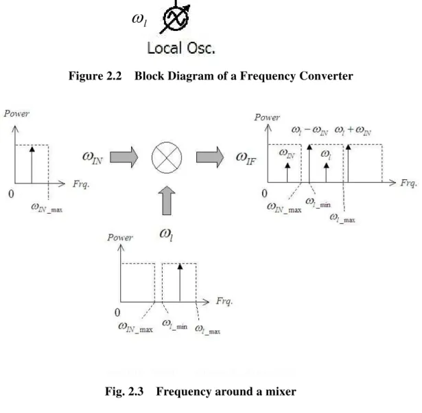
A block diagram of the Frequency converter is shown in Fig.2.2, which consists of three elements, a mixer, a local oscillator and an IF BPF (IF Band Pass Filter). The most important element is the mixer, which operates as a multiplier and makes the products of the input signal and the local oscillator as an analog circuit.

In the case that the frequency of the input signal and the local oscillator is ω_IN and ω_l, respectively, the mixer produce the two signals whose frequency are ω_IN +ω_l and |ω_IN −ω_l|. This operation corresponds to Eq.(2.1), which is one of the formulas about the trigonometric function [4].

[

^{cos( ) cos( )}

]

2 ) 1 cos( )

cos(A × B = A+B + A−B

.

(2.1)

And the output of the mixer includes two feed through factor of ω_IN and ω_l. These frequencies around the mixer are shown in Fig.2.3.

The ‘IF BPF’ permits only one signal, usually ω_IN +ω_l or |ω_IN −ω_l| to be outputted from the converter. The output of the IF BPF is called ‘IF (Intermediate Frequency) signal’.

In the case that the input signal f_IN(t) is explained as; )) ( cos(

) ( )

(t A t t t

f_IN = ω_IN +θ

,

(2.2)

the output will be

S_IF(t₎= A₍t_{)cos( (}ω_IN +ω_l)t+θ₍t₎₎ (2.3-a)

or

S_IF(t)= A(t)cos( |ω_IN −ω_l|t+θ(t))

,

(2.3-b)

where A(t) is the amplitude and ^θ (t) is the phase factor. The Frequency converter transform frequency only, and influences on other factors such as A(t) and θ(t).

Equation (2.3-a) and (2.3-b) can be explained by

S_IF

(

t

) = Re[

A

(

t

) exp[

j

( ( ω

_l

+ ω

_IN

)

t

+ θ (

t

))]]

(2.4-a)

or

S_IF

(

t

) = Re[

A

(

t

) exp[

j

( ( ω

_l

− ω

_IN

)

t

+ θ (

t

))]] .

(2.4-b)

The frequency ω_IN +ω_l or |ω_IN −ω_l | is generally called ‘Intermediate frequency’ or simply ‘IF’.

*) note: Sometimes a frequency converter is called another name such as down converter, frequency down converter, RF down converter and converter.

2.2.3 Input LPF

The discussion of last section has the assumption that the frequency of the input signal is under the frequency ω_{IN_max}which is lower than the lowest frequency of the local oscillator

mn

ωl _ . In the case that another signal exists and its frequency ω_IN' satisfies the following equation

IN l l

IN ^{ω ω ω}

ω '− = − , (2.5)

we cannot distinguish the frequency ω_IN from ω_IN'. To avoid this trouble, the input signal is passed through the LPF shown in Fig.2.1. The frequency ω_{IN_max} is the cut-off frequency of the LPF.

ω

IN

ω

_IF

ω

l

Figure 2.2 Block Diagram of a Frequency Converter

fin=2GHz, fl=6GHz, fl-fin=4GHz, fl+fin=8GHz

Fig. 2.3 Frequency around a mixer

- 17 -

2.3 Analog signal processing with swept local oscillator

The qualitative discussion on the frequency converters with swept local oscillator is given in this section.

2.3.1 Frequency converter with Swept Local Oscillator

In the condition that the local oscillator does not sweep and generate a CW signal, the system shown in Fig.2.2 operates as a general radio receiver. On the other hand, a sweep spectrum analyzer is provided with a characteristic that the local oscillator generates a sweeping signal. The frequency of output signal of the frequency converter is shown in Fig.2.4.

We assumed the system that is under the condition itemized as follows.

・The input is CW signal for simplification.

・The maximum and minimum frequency of the input signal is

ω

_{IN_max} and

ω

_{IN_min}.

・The minimum and maximum frequencies of the local oscillator,

ω

_{l_max} and ω_{l_min} which is defined as;

min _ max

_ l l

l

^{ω ω}

ω

≥ ≥ (2.6)

max _ min

_ max

_ l IN

l

^{ω ω}

ω

− =

.

(2.7)

・The frequency of the input signal is restricted by the input LPF as

IN

IN

^ω

ω

_{_max} ≥ . (2.8)

・The frequency of the local oscillator is higher than the frequency of the input.

max _ min

_ IN

l

^ω

ω

≥ (2.9)

・ ‘T_S’ is defined as the sweep time. The local oscillator generates the signal

ω

_l within the sweep time periodically. The time ‘t’ is considered periodically as

≥ 0

≥ t

T_S . (2.10)

Then the converter generates two signals, ω_l +ω_IN and ω_l −ω_IN, which are indicated in blue and red square in Fig. 2.4, respectively.

In the case that

ω

_IN equals to

ω

_{IN_min}, ω_IN +ω_l and ω_l −ω_IN are same frequency, and traced by the line ‘ ’ in Fig.2.4. Similarly,

ω

_IN equals to

ω

_{IN_max}they are traced by ‘ ’ and

‘ ’ respectively.

In the case of

ω

_IN =

ω

_{IN_min}, the frequency ω_IN +ω_l equals to

ω

_{l_max} at , which is indicated as the point ‘L’ in Fig.2-4.

TS

t

=

In the case that

ω

_IN =

ω

_{IN_max}, the frequency ω_l +ω_IN equals to

ω

_{l_max} at t

= 0

, which is

ω ω

+

ω

In the case that we configure the IF BPF whose center frequency equals

ω

_{l_min} or

ω

_{l_max}, we can obtain the power corresponding to the any frequency of

ω

_IN, and we can know the time when the power come in corresponds to the frequency

ω

_IN.

Frequency

max _ max

_ IN

l

^ω

ω +

max IN_

l

^ω

ω +

min _ max

_ IN

ω

l

+ ω

H M L

max _

ω

l

min _ max

_ IN

ω

l

− ω

IN

l

^ω

ω +

min _ IN

l

^ω

ω −

min _ IN

l

^ω

ω +

IN

l

^ω

ω −

L M H

min _

ω

l

max _ max

_ IN

l

^ω

ω −

max _

ω

IN

max _ IN

l

^ω

ω −

max _ min

_ IN

l

^ω

ω −

Time

2

S

/

0 T _T

_S

Fig. 2.4 Frequencies of signals around a mixer with the swept local

- 19 -

2.3.2 Output of IF BPF

The time-frequency diagram of the signal around the frequency converter with the swept local oscillator (see Fig.2.2) is shown in Fig.2.5. Where, the input signal is assumed as a single CW signal, the condition of the system is similar to that in the last section, and the center frequency of the IF BPF:ω_IF is set to

ω

_{l_min} (see Fig.2.4).

When the frequency of the mixer’s output is around

ω

_{l_min}, the output of the IF BPF has a power. The frequency ω_IF is generally called as ‘Intermediate Frequency’ or ‘IF frequency’.

The abscissa of Fig2.5 indicates the time and the ordinate indicates the frequency. The each graphs of the Fig.2.5 is itemized as follows.

- (a) shows the frequency of the input signal ^ωIN against time. The input signal is , which is assumed a single CW signal.

) (t f_IN

In his figure and (b) and (c), the ordinate indicates frequency.

- (b) shows the frequency of the local oscillator whose frequency is swept from ω_{l _START} to

STOP

ωl _ . These parameters satisfy the next equation.

min _ _

_ max

_ l STOP l START l

l ^{ω ω ω}

ω ≥ > ≥

- (c) shows the frequency of the mixer’s output, ω_{mix_out} =ω_l−ω_IN *) and the pass band of the IF BPF which is ω_IF =ω_{l_min}. ‘h(t)’ is the impulse response of the IF BPF. The frequency response of IF BPF is drawn as a graduated horizontal bar. By selecting the frequency ω_{l _START} and ω_{l _STOP} adequately, the line of ω_{mix _out} clothes the path band of the IF BPFaround the time t=T_S/2.

- (d) shows the output of the IF BPF as . In this figure, the ordinate indicates a voltage. The horizontal line indicates a voltage 0 V. Where has a significant value around

the time .

) S_IF(t

) S_IF(t 2

S/ T t=

- (e) shows the power of the . The unit of ordinate is dBm. We can consider is a spectrum of the input signal .

) (t

S_IF S_IF(t)

) (t f_IN

In the case that the input signal is another type of signal, such as modulated or multi CW signal etc, we can observe the spectrum of as a distribution of the spectrum.

) (t f_IN

) f_IN(t

In summary, for a sweep spectrum analyzer we should chose the IF frequency higher than the maximum frequency of the input signal ω_{IN_max} which corresponds to the cut-off of the LPF front of the mixer. The frequency of the local oscillator should be tuned from the IF frequency to the ‘IF frequency+ω_{IN_max}’ [1].

Frequency

Time

TS

t=

=0

t _t=0 t=T_S

Fig. 2.5 Time-Frequency diagram around a mixer with the swept local

Time

STOP

ωl _

ωIN

START

ωl _

ωl

)

Input Signal

(t

f_IN

⇔

)

(t

⇔

l Local Osc.

IN STOP

l ^ω

ω _{_} −

IN START

l ^ω

ω _{_} −

IN l out

mix ^{ω ω}

ω _{_} = −

min l_

IF

^ω

ω

=

^{⇔ h (t )}

IF BPF

)

(t

S

_IF

V

V

-

0V

(a)

(b)

(c)

(d)

(e)

2

S/ T t=

Output signal

⇔ of the mixer

dBm

- 21 -

2.3.3 Multi Conversion

Usually, spectrum analyzers have multiple frequency converters. Usually, they are called 1^st, 2^nd, and 3^rd converter from the front end of the input side. This section describes why spectrum analyzers have multiple down converters.

The frequency of the 1^st local oscillator in the most modern spectrum analyzer is approximately 4GHz to measure wide frequency range. The frequency resolution of the spectrum, which is obtained by the system in Fig.2.5, is decided by the bandwidth of the IF BPF. Some spectrum analyzer have the resolution 1kHz; others, 10Hz; still others, 1Hz. It is difficult to achieve such a narrow filter at the center frequency 4GHz. Therefore most spectrum analyzers typically have three or four stages of frequency converters [1]. The example of a multi stage of the frequency converter is shown in Fig.2.6. This example has three stages and the 3rd IF frequency is 21.4 MHz. Most spectrum analyzers have this IF frequency, 21.4 MHz and has the IF BPF as a resolution filter on this frequency.

Usually, the IF BPF on the 21.4MHz IF is called ‘Resolution Bandwidth Filter’, ‘RBW BPF’ or

‘RBW filter’, which decides the frequency resolution of the measure spectrum [1][2].

Note) The IF frequency of many FM radio receivers are 21.4MHz, and we can get the filter whose band pass is 21.4MHz with reasonable price. It is one of the reasons that the IF frequency of spectrum analyzers are 21.4MHz.

nd _d

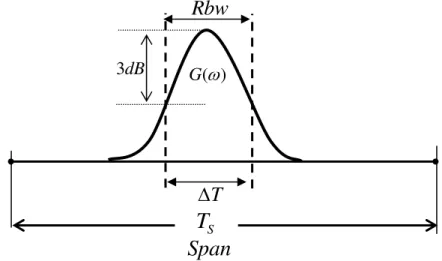
2.3.4 Restriction of Sweep time

A response of a RBW filter is illustrated in Figure 2.7, where the horizontal axis indicates both time and frequency. The measured signal is a CW, ‘Rbw’ is the 3dB bandwidth of the RBW filter; ‘T_S’ is the sweep time; ‘Span’ is the measurement frequency range which equals

START l STOP

l_ ^ω _

ω − ; and ‘ΔT’ is the time corresponding to the response of the RBW filter, which is explained as

Span T Rbw T

=

_S

×

Δ .

(2.11)

A sweep spectrum analyzer obtains the spectrum from the response of the RBW filter. Any filters require a finite time to charge and discharge, and the time length are inversely proportional to its bandwidth [1]. Then ΔT has a restriction explained by next equation.

Rbw T ≥ k⁰

Δ ,

(2.12)

where k₀ is a constant of proportionality. Equation (2.12) can be modified by replacing

Δ

T as the right side of Eq.(2.11).

Rbw

k

Span

T

_S

× Rbw ≥

⁰ . (2.13)

It is modified as

0 2

Rbw

k Span

T

_S

≥

. (2.14)

In the most sweep spectrum analyzers, the value of ‘k₀’ are in the range from two to three.

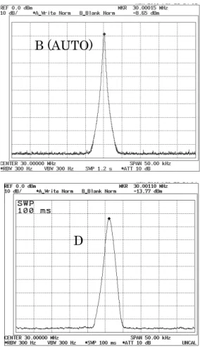
In the case that is shorter than the time of Eq.(2.14), the peak-level of the spectrum will be reduced as shown in Fig.2.8, where Span and Rbw of the all spectrums equal to 50 kHz and 300 Hz respectively. The sweep times of ‘A’ to ‘F’ is 2.0sec, 1.2sec, 500msec, 100msec, 50msec and 20msec, respectively. Especially, ‘B’ is a ‘AUTO’ which is configured by Eq.(2.14). The peak level is reduced and the width of the peak is expanded corresponding to the sweep rate, . We call this phenomenon ‘over sweep-rate response’.

TS

TS

TS

Span/ In the most conventional sweep spectrum analyzers, the value of is decided by a condition that the level reduction is about 0.1dB [2]. Actually, the difference level of peaks between A and B in Fig.2.8 was 0.13dB.

k0

In summary, sweep spectrum analyzer has a restriction on its sweep time and sweep rate.

- 23 -

Rbw

) (

ω

dB G

3

Δ T

St

Span

T

S

Fig 2.7 Response of an RBW filter measuring CW signal

2.3.5 Permissible distortion

The theory of level reduction is described in section 2.5. By the theory, we cannot measure a spectrum without any reduction. We have to use the analyzer permitting the level reduction, which is about 0.1dB [1][2].

Sweep spectrum analyzers have a property that the spectrum is shifted to the right side corresponding to the charge and discharge time of the RBW filter. Figure 2.8 shows the shifts that corresponds to the frequencies of the peaks as follows

Shift time = T_S^×{(frequency of the peak)- (center frequency)}/Span .

As the results, all of the shift times were approximately 2.2msec, which are 0.66 of the inverse of the Rbw= 300Hz.

In the case that the sweep time is longer than the condition of Eq.(2.14), as far as we observe the spectrum with our eyes, the shift and the level reduction is negligible obstruction.

2007.04.26, 2008.08.19

A ^{B (AUTO)}

C ^D

E F

Span=50kHz, Rbw=300Hz

Fig 2.8 Examples of over sweep-rate responses

- 25 -

2.4 Digital IF

The qualitative property of the sweep spectrum analyzer is described in section 2.2. The systems described in section 2.2 and 2.3 were analog type only. This section describes a ‘digital IF method’. We considered that introducing the digital IF method is appropriate to describe the property of the analyzers mathematically.

2.4.1 Digital IF method

The block diagram of Fig.2.9 suggests an example of the spectrum analyzer which has both analog and digital IF method. In the both method, the spectrum is measured as a changing power of the signal, ‘ ’, which is called as 'Intermediate frequency signal', or simply 'IF signal'. It is passed through the ‘IF BPF’ of the 3

) (t S_IF

rd down converter whose center of the pass band is fixed, as described in section 2.3.

In analog IF method, the IF signal is passed through the ‘LOG AMP’ and the power is detected by the ‘Detector’, and the ‘Video Filter’ reduced the bandwidth of the detected power, they are described in section 2.2. The ‘Peak Detector’ and the ‘Sampler’ pick up the extracted power at each interval, which is 1/500~1/4000 of the sweep time synchronized with the ‘Ramp signal’. The AD/C digitized the sampled power. Then the sampling frequency is satisfied 10kHz or 50kHz to detect the power.

In digital IF method, the AD/C digitizes the IF signal directory. In some early type of this method, the frequency of the IF signal were configured as the range under 10kHz and the sampling frequency were 20k or 30kHz. And a calculation of FFT (Fast Fourier transform) is used to obtain a spectrum [1].

In recent years (such as since 2000s), we can use high-speed AD/C with 14bit and digitize the 21.4MHz IF signal directly. In this thesis, the early type is not discussed. We will discuss about the type that has high-speed AD/C and signal processing devises. Figure 2.10 shows one example of a digital IF section which has high-speed AD/C and DDC (Digital Down converter described in chapter 4) and the DSP (may be any computer device). The details of the digital-IF method will be described, in following sections.

t S_IF

f

S

INPUT ^{S t}

t h BPF IF

NCIC

↓

FIR CIC

DDC ^{N N}

N = +

NFIR

↓

t jQ t I t

S_B = _B + _B

t

S

_IF

t

S

_q

!

! "# $ % &! '

t

t

t

A

t

S

_IF

= ω

_IF

+ θ

(

) ' A(t) ! ^θ(t) ! '

ω

_IF ' * + ! '

) t

S_IF ! ##$ # # ) $ , ' ' ' )

+ * ' ##$ ! ' -. ' ' '/ ' !

! -0 0 1 / -2$3/ ' ' ' ' )

IF

t

ω − ω

_IF

t

) & ' 4 !'

S

_IF

t

!

ω

_IF

t − ω

_IF

t

+ ) & ' 4 )

IF

t

ω

-I / -I ! ' / ' -I/ ! + 1 ' + ! ' 4 )

ω

_IF

t

-Q / -Q ! ' / ' -Q/

I ! ' ! , +

t t

t t

A t

I_q =

ω

_IF +

θ

×

ω

_IF 5

{

t t t

}

t A t

I_q =

ω

_IF +

θ

+

θ

5

1 ' + Q ! '

{ t t t }

t

A

t

t

t

t

A

t

Q

IF

IF IF

q

θ

θ

ω

ω

θ

ω

+

+

=

−

×

+

=

5

6 ' I_q t Q_q t ! &

t jQ t I t

S_q = _q + _q

) ' j '+ 6 ' , ' * + S_q t

" + ' S_q t -* ' ' '/ 6

* ' ' ' 78 ##$

! ' * + "# $ f_s ' * +

' ' ' f_s 9 ' ' * + ω_IF 2+* ' * + *

fs

π ! ' ) ' * + '

2+* ' * + ' ' , 2+* ' * + - /

t

S_q ! 78 ) $ $ : ' )

' ' $ $ : ' ' ! ' 9 ;(<

>

t

S

_B ' + ) ' ! ' '+ ! '

! ' ? ' ' ' ;5< )'

<

&!; t jQ t I

t j t A t

S

B B

B

+

=

=

θ

! At ! '

θ

t ! @*

t

t

t

A

t

f

_IN

= ω

_IN

+ θ

@* (

t

t

t

A

t

S

_IF

= ω

_IF

+ θ

) , ' ' , ' = '' '

' * + ' ! ! +!

S

_B

t

' +

" "

6 ' f_IN t S_IF t ' ' ! ' + " )

+

<

&!;

A

^{t A t j t t}

f

_{IN A}

= × ω

_IN

+ θ

>

<

&!;

A

^{t A t j t t}

S

_{IF A}

= × ω

_IF

+ θ

>

+ ' = '' ' ' * + ' f_INAA t S_IFAA t

' * + ' S_B t + 78 ) ' !

' * + B + ##$ ' ' )

' + ' $ $ : ' )

'

N

_CIC

N

_FIR ! + '

N

_DDC

FIR CIC

DDC

^{N N}

N = +

s 9

f

! _{fs 9 fs −fs 9 −fs}

! ! "" ! S_B t #$% ! !

! & ! ' !!

! ( ! ! "

! )*+ ! !

, ! - ../ ( !

! ( !

。

! #

$ % % &

' ) ! ! ' +% ' ' ) ! l(t) )

&!

[ ]

&! π⋅σ +ω +θ

= j t t

t l

S

S ^{t T}

T ≤ ≤

−

) ' t ) ! ' ω ' * + t=0

θ

!

0 ! !

1 1 !

2

. 1 1

! 2

9 fS

9 fS

−

t

S

_B

t

S

_q

t S_IF

DDC

ω

H

IF

fS _=ω

9

C

t t t

A t

f_IN =

ω

_IN +

θ

! ) , ' ' S t > ' & * +

C

[ ]

[ ^{&!; <} ]

:

<

&!;

:

θ

θ

ω

ω

σ

π

θ

ω

+

+

−

+

×

×

=

×

+

−

×

×

=

t

t

t

j

t

A

a

t

l

t

t

j

t

A

a

t

S

IN l IN

) ' -a/ * , ) + +

! "# $ ) ! & ! ' '' '

' * +

[

^{&!; <}

]

:

D

× × π σ + ω + θ + θ

=

a At j t t t

t

S_{IF IF} C

) ' a’ ) '' ! ) , ' '

ω

_IF

ω

IFE

ω

_l

− ω

_IN

* C ) 08 ) , ' '

' + ) ' ) 8' +

08 ' @* C ' )'

[ ]

{

^D

^{× ×}

^{: &!;}

^{π σ + ω + θ + θ}

^<

}

∗

=

h t a A t j t t t

t

S_{IF IF} C

) ' h t ! ' ! 08

ω

_IF ' ' * +

08 " + h t ' ! '' ) 08 + 08

) , ' ' > 08 C^' ) , ' ' @* C

, t ' ' , ' * + ' "

!

S

_IF

t

' ) F F ' '

' & ! % ) ! ' @* C

) '

ω

_IF * 9G?%

θ

t

θ

* % ' ' ! 1! *

G?% 1) ! * + ' * +

'' ' * +

ω S

_IF

t

' ! @* C

) &!

IF

^πσ t

ω

ω = +

9

) ' + @*

! ' ' ' '' !

' * + ' ! ' h t

) h t ) !!' & + G?% 6 ! '

t

f_IN + ! ) ' ) ) 0 '' ) '

! ' ' ' ! ' , + !'

% ) ' )

' S

_IF

t

G ' ) $6 SpanE G?% T_SE 0 ) ≒ G?%

%

! ' +% ' ) + ) > '

t

S_IF ! ' "# $ ##$ , '

) ' !' S_B t @* & ! S_B t )

C ) , ' ' S_IF t @* C

2$3 ##$ ' ω_IFt −

ω

_IFt ' * + '

ω

_IF

' = S_B t &!

{

^{H× × &!; π σ +θ +θ <}

}

∗

= h t a A t j t t

t

S_{B DDC} (

) ' a” '' ! + h_DDC t ! ' !

78 ! ##$ B + ) h_DDC t '' ) ' h(t) in

@* C ' * + ' ! h_DDC t ' ) H_DDC ω 6 '

C 0 ) H_{DDC ω} h_DDC t ' 9G?%

' * + S_B t ' ! ' @* ( &!

d

_θ

σ

π

ω

= + ⁵

MHz

CC

$ ! % " &( ' S

_B

t

G ' ) $6 SpanE G?% T_SE 0 ) ≒9G?%

' * +

ω

_B ?% ) * % ' ) , '' ) ' 78

t

S

_B ) & ' ! ' ' ?% ! ' ! ) 9 2 )

) '' ) 78 -) * + ! S_BARBW t

' * + ! ω_IN ±δω ' * +

δω

σ

π

ω

_Bδ

=

t

±

t )

ω

_Bδ * % ' &!

t t

σ

π

=

δω

t '' ! ' * + δω δω &!

σ

t

π

δω

=

6 ' ! ' ! + ' '

C 9 ' * + 6

! ) ' ! ' + ! * ' ' ! ' '+ ! ' S_BARBW t

) & ! ) (

! ' + ) *

(

^S A ^t

) (

^{I t Q t}

)

F ω = _{B RBW} = +

MHz