Constraints on the neutrino parameters by future
cosmological 21cm line and precise CMB polarization
observations
Yoshihiko Oyama
DOCTOR OF PHILOSOPHY
Department of Particle and Nuclear Physics
School of High Energy Accelerator Science
The Graduate University for Advanced Studies (SOKENDAI)
2014
Abstract
Observations of the 21 cm line radiation coming from the epoch of reionization have a great capacity to study the cosmological growth of the Universe. Also, CMB polarization produced by gravitational lensing has a large amount of information about the growth of matter fluctuations at late time. In this thesis, we investigate their sensitivities to the impact of neutrino property on the growth of density fluctuations, such as the total neutrino mass, the neutrino mass hierarchy, the effective number of neutrino species (extra radiation), and the lepton asymmetry of our Universe.
We will show that by combining the precise CMB polarization observations with Square Kilometer Array (SKA) we can measure the impact of non-zero neutrino mass on the growth of density fluctuation, and determine the neutrino mass hierarchy at 2 σ level if the total neutrino mass is smaller than 0.1 eV.
Additionally, we will show that by using these combinations we can constrain the lepton asymmetry better than big-bang nucleosynthesis (BBN). Besides we discuss constraints on that in the presence of some extra radiation, and show that the 21 cm line observations can substantially improve the constraints obtained by CMB alone, and allow us to distinguish the effects of the lepton asymmetry from those of extra radiation.
Contents
1 Introduction 4
1.1 Observations of 21 cm line radiation . . . 4
1.2 21 cm line . . . 5
1.3 Neutrino mass and its properties . . . 5
1.4 Purposes and organization of this thesis . . . 7
1.5 Basic variables and constants . . . 8
2 Brightness temperature of 21 cm radiation 11 2.1 Brightness temperature and transfer equation . . . 11
2.1.1 Brightness temperature . . . 11
2.1.2 Transfer equation . . . 12
2.1.3 Emission and absorption coefficients in a two level system . . . 12
2.1.4 Spin temperature . . . 14
2.1.5 The solution of the transfer equations . . . 14
2.2 Optical depth and line profile . . . 16
2.2.1 Optical depth . . . 16
2.2.2 Line profile . . . 16
2.3 Observed brightness temperature . . . 19
3 Spin temperature 21 3.1 Time evolution of the spin temperature . . . 21
3.1.1 The evolution equation of spin temperature . . . 21
3.1.2 Spin temperature in thermal equilibrium . . . 27
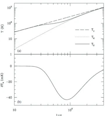
3.2 Global history of the spin temperature . . . 28
3.2.1 Before the star formation 30 <∼ z <∼ 300 : The dark age . . . 28
3.2.2 After star formation z <∼ 30 : The cosmic dawn and the epoch of reionization . . . 28
4 Fluctuation and power spectrum of the 21 cm radiation 32 4.1 Fluctuation of brightness temperature . . . 32
4.1.1 Fluctuation of brightness temperature . . . 32
4.1.2 In the case of Tγ << TS . . . 34
4.2 Power spectrum of 21 cm line radiation . . . 34
4.2.1 Power spectrum of 21 cm line radiation . . . 34
4.2.2 Power spectrum of ionization fraction . . . 36
5 Density fluctuations and neutrino properties 38 5.1 Density fluctuations . . . 38
5.1.1 Equations of density fluctuations . . . 38
5.1.2 Equations of matter fluctuations . . . 41
5.2 Free-streaming behavior of neutrinos . . . 42
5.2.1 Free-streaming length . . . 42
5.2.2 Large scale behavior of neutrinos . . . 43
5.2.3 Small scale behavior of neutrinos . . . 46
5.3 Peculiar velocity . . . 48
5.4 Other effects due to neutrino properties . . . 50
5.5 Influence of lepton asymmetry of the Universe . . . 51
5.5.1 Background . . . 51
5.5.2 Perturbation equation . . . 54
6 Fisher information matrix 55 6.1 Fisher information analysis . . . 55
6.1.1 Definition of statistical quantities . . . 55
6.1.2 Variance-covariance matrix . . . 56
6.1.3 Unbiased estimator . . . 56
6.1.4 Fisher information matrix . . . 57
6.1.5 Cram´er-Rao bound . . . 57
6.2 Fisher information matrix for Gaussian likelihood . . . 60
7 Fisher information matrix of 21 cm line observation 63 7.1 Visibility . . . 63
7.1.1 Definition of visibility . . . 63
7.1.2 Visibility for a narrow radio source . . . 65
7.1.3 Visibility of 21cm line observations . . . 67
7.2 Fisher information matrix of 21 cm line observations . . . 69
7.2.1 Sample variance . . . 70
7.2.2 Detector Noise . . . 72
7.2.3 Contribution of residual foregrounds . . . 73
7.2.4 Total variance-covariance matrix CSTb . . . 75
7.2.5 Relation between P21(u) and P21(k) . . . 76
7.2.6 Fisher matrix of 21 cm line observations . . . 77
7.3 Specifications of the experiments . . . 79
8 Fisher information matrix of cosmic microwave background (CMB) 81
8.1 CMB and neutrino properties . . . 81
8.2 Fisher information matrix of CMB . . . 81
8.3 Residual foregrounds . . . 83
8.4 Specifications of the experiments . . . 84
8.4.1 Analysis of the neutrino mass and the mass hierarchy . . . 84
8.4.2 Analysis of the lepton asymmetry . . . 84
9 Fisher information matrix of baryon acoustic oscillation (BAO) observa- tions 87 9.1 Fisher matrix of BAO . . . 87
9.2 Specification of the BAO observation . . . 88
10 Forecasts for the neutrino mass 90 10.1 Future constraints . . . 90
10.2 Constraints on Σmν and Nν . . . 91
10.3 Constraints on the neutrino mass hierarchy . . . 97
11 Forecasts for the lepton asymmetry 99 11.1 Cases without extra radiation . . . 102
11.2 Cases with extra radiation . . . 103
12 Summary 111 A Hyperfine splitting of neutral hydrogen atom 114 B Einstein coefficients 117 C Non-relativistic limit of ρν + ρν¯ 119 C.1 Expressions for the coefficients Ci . . . 119
C.2 Non-relativistic limit of ρν+ ρν¯ and pν + pν¯ for any ξ . . . 120
D BBN relation 121
Chapter 1
Introduction
1.1 Observations of 21 cm line radiation
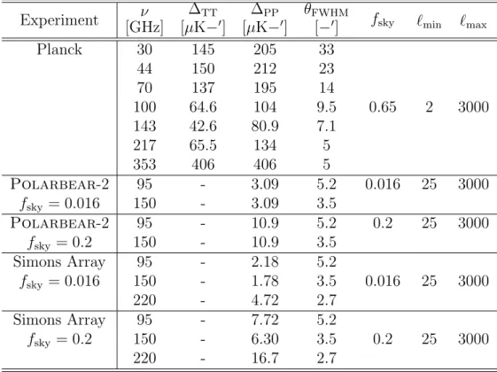
Observations of high-redshift Universe (6 <∼ z) with the 21 cm line of neutral hydrogen attracts attention because it opens a new window to the early phases of the cosmological structure formations. After recombination (z ∼ 1100), because the Universe is neutral, and there had not existed any luminous objects yet, this era is called “the cosmic dark age”. After the dark age, first luminous objects formed at around z ∼ 30, and this epoch is called “the cosmic dawn” or just “ the late time of the dark age”. Finally X-rays are emitted from the remnants of the luminous objects, which ionizes the inter-galactic medium (IGM). This epoch is called “the epoch of reionization (EOR)”. So far, it has been a big challenge to observe such past epochs. However, there are a lot of hydrogen gas in the IGM. Therefore we can observe them by using the 21 cm line which are emitted by them (Fig.1.1). This is the reason why the observation of the 21 cm line attracts attention quite recently.
Using the observation of the 21 cm line, we can study not only how the Universe was ionized, but also we can obtain information about the density fluctuations of matter because the distribution of neutral hydrogen traces that of cold dark matter (CDM). Therefore, we can use the observation of the 21 cm line like those of CMB or Galaxy surveys, and constrain cosmological parameters such as the density parameter for the energy density of CDM Ωc or of dark energy ΩΛ. Besides, the observation of the 21 cm line has some advantages. First, the observation enables us to survey very past eras and wide redshift ranges (21 cm tomography). Secondly, in such a high redshift era, the non- linear growth of the fluctuation is smaller than that in later epochs. Therefore theoretical uncertainties of the predictions for the 21cm line observations is much smaller than that for galaxy surveys.
First star CMB
formation Full
reionization
Dark age Cosmic
dawn Epoch of
reionization
: Number density of neutral hydrogen : Number density of hydrogen
: Neutral fraction
Recombination
(neutralization of Universe) Signals of 21 cm line exist
Figure 1.1: Epochs in which cosmological 21 cm line was emitted.
Spin =0 singlet Spin =1 triplet
proton
electron
eV cm
1S state
Hyperfine splitting
Figure 1.2: Hyperfine structure of neutral hydrogen atom.
1.2 21 cm line
The 21 cm line of neutral hydrogen atom is emitted by transition between the hyperfine levels of the 1S ground state, and the hyperfine structure is induced by an interaction of magnetic moments between proton and electron (see Appendix A). The energy difference of the hyperfine structure is ∆E ∼ 5.8 × 10⁻⁶eV, and this energy corresponds to the frequency ν21 ≃ 1.4GHz (the wave length is λ ≃ 21cm). Therefore this spectral line is called the 21 cm line (see Fig.1.2).
1.3 Neutrino mass and its properties
Due to the discovery of non-zero neutrino masses by Super-Kamiokande through neutrino oscillation experiments in 1998, the standard model of particle physics was forced to be modified so as to theoretically include the neutrino masses.
So far only the mass-squared differences of neutrino species have been measured by neutrino oscillation experiments, which are reported to be ∆m221≡ m22− m21 = 7.59+0.19−0.21× 10⁻⁵eV2 [1] and ∆m232 ≡ m23 − m22 = 2.43+0.13−0.13 × 10⁻³eV2 [2]. However, absolute values and their hierarchical structure (normal or inverted) have not been obtained yet although information on them is indispensable to build new particle physics models.
In particle physics, some new ideas and new future experiments have been proposed to measure the absolute values and/or determine the hierarchy of neutrino masses, e.g., through tritium beta decay in KATRIN experiment [3], neutrinoless double-beta decay [4], atmospheric neutrinos in the proposed iron calorimeter at INO [5, 6] and the upgrade of the IceCube detector (PINGU) [7], and long-baseline oscillation experiments, e.g., NOνA [8], J-PARC to Korea (T2KK) [9, 10] or Oki island (T2KO) [11], and CERN to Super-Kamiokande with high energy (5 GeV) neutrino beam [12].
On the other hand, such non-zero neutrino masses affect cosmology significantly through suppression of growth of density fluctuation because relativistic neutrinos have large large thermal velocity and erase their own density fluctuations up to horizon scales due to their free streaming behavior. By measuring power spectra of density fluctuations, we can con- strain the total neutrino mass Σ mν [13–30] and the effective number of neutrino species Nν [13–17, 20, 21, 30–32] through observations of cosmic microwave background (CMB) anisotropies and large-scale structure (LSS). The robust upper bound on Σ mν obtained so far is Σmν < 0.23 eV (95 % C.L.) by the CMB observation by Planck (see Ref. [30]). For forecasts for future CMB observations, see also Refs. [33–36].
Moreover, by observing the power spectrum of cosmological 21 cm line radiation fluctu- ation, we will be able to obtain useful information on the neutrino masses [37–42]. That is because the 21 cm line radiation is emitted (1) long after the recombination (at a redshift z ≪ 103 ) and (2) before an onset of the LSS formation. The former condition (1) gives us information on smaller neutrino mass ( ≲ 0.1 eV), and the latter condition (2) means we can treat only a linear regime of the matter perturbation, which can be analytically calculated unlike the LSS case.
In actual analyses, it is essential that we combine data of the 21 cm line with those of CMB because the constrained cosmological parameter space is complementary to each other. For example, the former is quite sensitive to the dark energy density, but the latter is relatively insensitive to it. On the other hand, the former has only a mild sensitivity to the normalization of matter perturbation, but the latter has an obvious sensitivity to it by definition. In pioneering work by [39], the authors tried to make a forecast for constraint on the neutrino mass hierarchy by combining Planck with future 21 cm line observations in case of relatively degenerate neutrino masses Σmν ∼ 0.3 eV.
Additionally, there is another issue related to the neutrino properties, it is the lepton asymmetry of the Universe. The issue of the asymmetry of matter and antimatter in the Universe is one of the important subject in cosmology and particle physics. The baryon asymmetry is now accurately determined by using the combination of cosmological obser- vations such as cosmic microwave background (CMB), big bang nucleosynthesis (BBN), large scale structure, type Ia supernovae and so on. It is represented in term of the baryon-
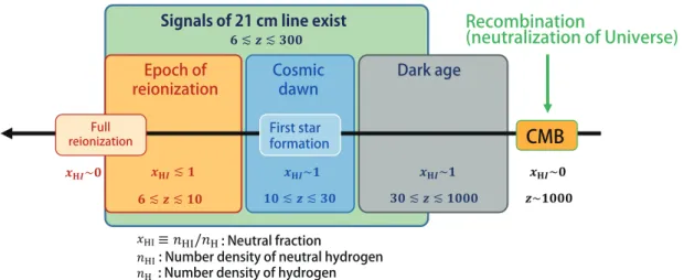
Figure 1.3: An image of the Square Kilometer Array (SKA) http://www.skatelescope.org/
photon ratio η = (nb − n¯b)/nγ ≃ 6 × 10⁻¹⁰, where nb, n¯b and nγ are the number densities of baryon, anti-baryon and photon, respectively. On the other hand, the asymmetry in the leptonic sector is not well determined and only a weak constraint on the neutrino degeneracy parameter ξν = µν/Tν is obtained #1. Although the lepton asymmetry is ex- pected to be the same order as the baryon asymmetry due to the spharelon effect, in some models, it can be much larger than the baryonic asymmetry [48–52]. Furthermore, if the lepton asymmetry is large, it may significantly affect some aspects of the evolution of the Universe: QCD phase transition [53], large-scale cosmological magnetic field [54], density fluctuations if primordial fluctuation is generated via the curvaton mechanism [55–57] and so on.
Thus, it would be worth investigating to what extent the lepton asymmetry can be probed beyond the accuracy of current cosmological observations. Since the signals from the 21 cm line can cover a wide redshift range, they can be complementary to other observations such as CMB. In addition, the effects of the lepton asymmetry mainly appear on small scales, which can be well measured by 21 cm line observations. Thus such a survey would provide useful information.
1.4 Purposes and organization of this thesis
In this thesis, we focus on future observations of both the 21 cm line radiation coming from the epoch of the reionization (7 ≤ z ≤ 10) and the CMB polarization produced by a gravitational lensing, in order to study their sensitivities to the neutrino properties such as the total neutrino mass, the neutrino mass hierarchy, the effective number of neutrino species (extra radiation component), and the lepton asymmetry of our Universe. As 21 cm line observation, we particularly focus on future experiments such as the Square Kilometer
#1So far constraints on ξν have been obtained by BBN (e.g., see [43, 44] and Fig. D.1 in Appendix D), which is sometimes combined with CMB and/or some other observations (e.g., see Refs. [45–47]).
Array (SKA) (Fig.1.3) [58] and Omniscope [59, 60].
This thesis is organized as follows. In Chapter 2, 3 and 4, we review the brightness temperature of the 21 cm radiation, the spin temperature (excitation temperature of the hyperfine splitting), and the power spectrum of the 21 cm radiation, respectively. In Chapter 5, we briefly explain the growth of the density fluctuations and some effects due to neutrino properties. In Chapter 6, 7, 8 and 9, we summarize our analytical methods (Fisher information analysis), and review Fisher matrices of each experiment (21 cm line, CMB and BAO (baryon acoustic oscillation), respectively). In Chapter 10, and 11, we present our results as forecasts for specific observations, paying particular attention to how the 21 cm observations will help to measure neutrino parameters.
1.5 Basic variables and constants
Here, we present a summary table of basic symbols in this thesis. Symbol Definition
a Scale factor.
Aul Einstein A coefficient (spontaneous decay rate). A21 Einstein A coefficient of the hyperfine splitting. Bul Einstein B coefficient (stimulated emission). Blu Einstein B coefficient (absorption).
c Light speed.
fν Energy fraction of neutrino to matter, fν ≡ ρν/(ρb + ρc+ ρν), where ρν includes both of neutrino and anti-neutrino.
gu Degree of freedom of the upper state. gl Degree of freedom of the lower state. g0 Degree of freedom of the spin singlet state. g1 Degree of freedom of the spin triplet state. gµν Metric tensor.
H Hubble parameter, H ≡ (da/dt)a−1, where t is the cosmic time. H Conformal Hubble parameter, H = aH.
H0 Present value of the Hubble parameter.
h Dimensionless Hubble parameter, h ≡ H0/(100km s−1 Mpc−1). hP Planck constant.
ℏ Reduced Planck constant, ℏ ≡ hP/2π.
Iν Specific intensity.
IνBB Specific intensity of black body.
k Wave number vector (Fourier dual of the comoving coordinate). k Absolute value of k, k = |k|.
kB Boltzmann constant. me Electron mass. mH Hydrogen mass.
Symbol Definition mν Neutrino mass.
Σmν Total neutrino mass, Σmν ≡∑3i=1mi, where mi is each mass eigenstate. Nν Effective number of neutrino species.
∆Nν Difference between the effective number of neutrino species. and the standard value, ∆Nν ≡ Nν− 3.046.
p Pressure.
P21 Power spectrum of δ21 (21 cm line power spectrum). Pδδ Power spectrum of matter density fluctuation.
T Temperature.
Tb Brightness temperature.
tg Proper time of a radiation source. TS Spin temperature.
Tγ CMB temperature. w w ≡ p/ρ.
Yp Helium fraction. xHI Neutral fraction
(the ratio of neutral hydrogen atoms and total protons). xi Ionization fraction, xi = 1 − xHI.
z Redshift, z = a−1− 1. αEM Fine structure constant.
δ Density fluctuation. δ21 Fluctuation of ∆Tbobs.
δb Density fluctuation of baryons.
δc Density fluctuation of cold dark matter. δD(x) Dirac delta function.
δH Density fluctuation of hydrogen. δHI Density fluctuation of neutral fraction.
δν Density fluctuation of neutrinos.
∆Tb Difference between the 21 cm line brightness temperature and CMB temperature, Tb− Tγ.
∆Tbobs observed ∆Tb. η Conformal time. λ Wave length.
λ21 Wave length of 21 cm line.
µ Cosine of the angle of a wave vector between a line of sight direction. µνi Chemical potential of each neutrino flavor νi.
ν Frequency.
ν21 Frequency of 21 cm line at a rest frame.
νul Transition frequency between the upper and lower state. ξ Degeneracy parameter.
Symbol Definition
ξνi Degeneracy parameter of each neutrino flavor, ξνi ≡ µνi/Tν. ρ Energy density.
ρb Energy density of baryons.
ρc Energy density of cold dark matter.
ρm Energy density of matter, ρm ≡ ρc+ ρb + ρν. ρν Energy density of neutrinos.
In the section 5.5 and the appendix C,
ρν includes only the energy density of neutrino.
In the other chapters and sections, it includes both of neutrino and anti-neutrino.
τν Optical depth.
ϕ(η, x) Perturbation of gravitational potential, where x is the comoving coordinate. ψ(η, x) Perturbation of spatial curvature,
where x is the comoving coordinate. Ωb Density parameter of baryons at present. Ωm Density parameter of matter at present. ΩΛ Density parameter of dark energy at present. Ων Density parameter of neutrino at present.
Chapter 2
Brightness temperature of 21 cm
radiation
[61–63]In this chapter, we review basic physical quantities about the cosmological 21 cm line observation. For further details, we refer the readers to Refs. [61, 62].
2.1 Brightness temperature and transfer equation
[64,65]
2.1.1 Brightness temperature
Brightness temperature Tb means intensity of radiation, and it is defined by specific inten- sity of black body in the Rayleigh-Jeans approximation (kBT >> hPν). In the approxi- mation, the specific intensity of black body IνBB is given by
IνBB(T ) = 2ν
2
c2 kBT. (2.1)
By using the specific intensity of black body IνBB, the brightness temperature Tb is defined as
Iν = 2ν
2
c2 kBTb
−→ Tb ≡ c
2
2ν2kB
Iν, (2.2)
where Iν is intensity of radiation (specific intensity : emitted energy per unit area, unit time, unit frequency and unit solid angle).
When the Rayleigh-Jeans approximation is not applicable, the specific intensity of black body IνBB is given by
IνBB(T ) = 2hPν
3
c2
1 exp(khPν
BT
)− 1. (2.3)
Therefore, we can define the equivalent brightness temperature Jν(T ) as Jν(T ) ≡
hν kB
1 exp(khPν
BT
)
− 1
(2.4)
−→ Iν = 2ν
2
c2 kBJν(T ). (2.5)
From now on, we do not distinguish Jν(T ) from Tb, and express them as just Tb.
2.1.2 Transfer equation
The flux intensity obeys the transfer equation, 1
c
dIν(r, t, n)
dt = ην(r, t, n) − αν(r, t, n)Iν(r, t, n), (2.6) where t is the cosmic time , ην is the emission coefficient, which represents the contribution of spontaneous emission, αν is the absorption coefficient, which represents the contribution of absorption and stimulated emission (it is interpreted as negative absorption), r is the comoving coordinate, and n is the unit vector which points to the direction of radiation.
Here, we define the optical depth τν as, dτν ≡ ανcdt = ανds ←→ τν(s) ≡
∫ s 0
αν(r(s′), s′, n(s′))ds′, (2.7) where s is the physical length. This quantity τν represents the degree of diffusion of radiation. By using a transformation of t −→ τν, the transfer equation becomes
dIν(r, τν, n) dτν = −I
ν(r, τν, n) + ην(r, τν, n)
αν(r, τν, n), (2.8) and we can rewrite this equation as the following equation relevant to the brightness temperature Tb,
dTb(ν, r, τν, n)
dτν = −Tb
(ν, r, τν, n) + c
2
2kBν2
ην(r, τν, n)
αν(r, τν, n). (2.9) By solving this equation, we can get the solution of brightness temperature Tb.
2.1.3 Emission and absorption coefficients in a two level system
In this subsection, we discuss a two-level system because the hyperfine structure is de- scribed by such a system. In the two-level system, the emission and absorption coefficients are expressed by the Einstein A and B coefficients, which represent the probability of a transition between two energy levels. The A coefficient corresponds to the spontaneous emission, and the B coefficient corresponds to the absorption and the stimulated emission, respectively.
A coefficient : Aul
The Einstein coefficient Aul represents the probability of a transition between two energy levels per unit time. The unit is inverse of time.
B coefficients : Blu, Bul
The probability of absorption and stimulated emission are proportional to the intensity of incoming radiation. Therefore, we introduce the average intensity ¯J,
J ≡¯ 4π1
∫
4π
dΩ
∫ ∞
0
Iνϕ(ν)dν, (2.10)
where ϕ(ν) is a line profile, and by using ¯J, we define the Einstein B coefficients as BluJ : The probability of absorption,¯
BulJ : The probability of stimulated emission.¯
These coefficients are related to the variation of intensity, and the relations are expressed as
Spontaneous emission : dIν = hPνul
4π nuϕe(ν)Aulcdt, (2.11a) Absorption : dIν = hPνul
4π nlϕa(ν)BluIνcdt, (2.11b) Stimulated emission : dIν = hPνul
4π nuϕe(ν)BulIνcdt. (2.11c) Here, nl(r, t) and nu(r, t) are the number density of atom in the lower state and the upper state, respectively, ϕe(ν) and ϕa(ν) are the line profiles of emission and absorption, respectively. Therefore, the equation of intensity Iν can be written as
dIν = dIν |Spontaneous +dIν |Absorption +dIν |Stimulated
−→ 1 c
dIν
dt = hPνulnuϕe Aul
4π − hPνul {
nl
Blu
4πϕa− nuϕe Bul
4π }
Iν, (2.12) where νul is the transition frequency between the upper and lower states. In comparison between (2.6) and (2.12), we can express the emission and absorption coefficients as
ην(r, t) = hPνulnu(r, t)ϕe(ν)Aul
4π (2.13a)
αν(r, t) = hPνul
{
nl(r, t)Blu
4πϕa(ν) − nu(r, t) Bul
4πϕe(ν) }
. (2.13b)
In this situation, αν and ην do not depend on the direction of radiation n. From now on, we assume that the line profiles of emission and absorption are same function (ϕ(ν) ≡ ϕa(ν) = ϕe(ν)) for simplicity.
2.1.4 Spin temperature
We introduce the spin temperature TS, which is the excitation temperature of hyperfine structure (the detail is shown in the Chapter 3),
nu
nl ≡
gu
gl
exp (
−hPνul kBTS
)
, (2.14)
where gu and gl are the degree of freedom of the upper and lower states, respectively. According to the following relation (the detail is shown in the Appendix B)
Aul = 2hPν
ul3
c2 Bul, (2.15a)
guBul = glBlu, (2.15b)
we can express αν as
αν = hPνul
4π ϕ(ν)nlBlu {
1 −nnu
l
Bul
Blu }
= c
2
8πνul2 gu
gl
Aulnlϕ(ν) {
1 − exp (
−hPνul kBTS
)}
. (2.16)
Therefore, the source term of Eq.(2.9) (the second term on the right hand side) can be written as
ην
αν
= hPνulnuϕe(ν)Aul 4π
[ c2 8πνul2
gu
gl
Aulnlϕ(ν) {
1 − exp (
−hPνul kBTS
)}]−1
= 2hPν
3 ul
c2 gl gu
nu nl
{
1 − exp (
−hkPνul
BTS
)}−1
= 2hPν
ul3
c2
1 exp(hkPνul
BTS
)
− 1
≈ 2ν
2 ul
c2 kBTS. (2.17)
In the last line, we use the approximation of hPνul << kBTS. This approximation is valid in observations of 21 cm line because hPνlu/kB ≃ 0.068K and generally 0.068K << TS (the detail is shown in the Chapter 3).
2.1.5 The solution of the transfer equations
By using Eq.(2.17), we can rewrite Eq.(2.9) as dTb(ν, r(τν), τν)
dτν = −Tb
(ν, r(τν), τν) +(νul ν
)2
TS(r(τν), τν). (2.18)
The solution of Eq.(2.18) is given by
Tb(ν, r(τν), τν) = e−τνTb(ν, r(0), 0) +(νul ν
)2∫ τν 0
eτν′−τνTS(r(τν′), τν′)dτν′. (2.19) By using approximation of TS(r(τν′), τν′) ≈ TS(r(0), 0), we can rewrite Eq.(2.19) as
Tb(ν, r(τν), τν) ≈ e−τνTb(ν, r(0), 0) +(νul ν
)2
TS(r(0), 0)[1 − e−τν] . (2.20) Therefore, the difference between the brightness temperature Tb(ν, r(τν), τν) and the in- coming radiation Tb(ν, r(0), 0) can be written as
∆Tb(ν, r(0), 0) ≡ Tb(ν, r(τν), τν) − Tb(ν, r(0), 0)
≈(1 − e−τν) [(νul
ν )2
TS(r(0), 0) − Tb(ν, r(0), 0) ]
. (2.21) Here, the brightness temperature of incoming radiation Tb(ν, r(0), 0) is that of CMB radi- ation Tγ. By the comoving coordinate r(0) at the incident point and the conformal time η(z) at the point, the temperature of incoming radiation Tb(ν, r(0), 0) can be expressed as Tb(ν, r(0), 0) = Tγ(r(0), η(z)). (2.22) From now on, by the comoving coordinate r(0) and the conformal time η(z), we express the spin temperature and ∆Tb to be TS(r(0), η(z)) and ∆Tb(ν, r(0), η(z)), respectively.
Because the observed brightness temperature is redshifted (the frequency and the tem- perature of CMB rise 1/(1 + z)-fold), the difference of observed brightness temperature
∆Tbobs is given by
∆Tbobs ( ν
1 + z, r(0), η(z) )
= ∆Tb(ν, r(0), η(z)) 1 + z
= (νul
ν
)2
TS(r(0), η(z)) − Tγ(r(0), η(z))
1 + z (1 − e
−τν) .(2.23)
In the case of ν = νul, ∆Tbobs is expressed as
∆Tbobs ( νul
1 + z, r(0), η(z) )
= TS(r(0), η(z)) − Tγ(r(0), η(z))
1 + z (1 − e
−τνul) . (2.24)
From Eq.(2.24), when the spin temperature TS is higher than the CMB temperature Tγ, the observed radiation becomes an emission line (0 < ∆Tbobs). By contrast, when TS is lower than Tγ, the observed radiation becomes absorption line (∆Tbobs < 0). From now on, the “difference of the brightness temperature ∆Tbobs” is called just the “brightness temperature”.
φ νul
νul ν
᷀ν φ ν
Figure 2.1: Line profile
2.2 Optical depth and line profile
2.2.1 Optical depth
In this section, we estimate the optical depth τνul, which appears in Eq.(2.24). The optical depth is defined by Eq.(2.7) to be,
τν(r(s), r(0), η(z)) =
∫ s 0
αν(r(s′), s′, η(z))ds′. (2.25) By using Eqs.(2.16), (2.25) and the approximation of hνul << kBTS, the absorption coefficient αν is expressed as
αν(r, η) = c
2
8πνul2 gu
gl
Aulnl(r, η)ϕ(ν) {
1 − exp (
−k hPνul
BTS(r, η) )}
≈ c
2
8πνul2 gu
gl
Aulnl(r, η)ϕ(ν) hPνul
kBTS(r, η). (2.26)
Therefore, the optical depth is given by τν(r(s), r(0), η(z)) = c
2h PAul
8πkBνul
gu gl
ϕ(ν)
∫ s 0
nl(r(s′), η(z)) 1
TS(r(s′), η(z))ds
′. (2.27)
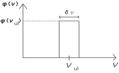
2.2.2 Line profile
In this subsection, we estimate the line profile ϕ(ν) in Eq.(2.27). The line profile is normalized as follows,
∫ ∞
0
ϕ(ν)dν = 1. (2.28)
We can consider that ϕ(νul) has non-zero value between only δν which is the frequency region near the transition frequency νul (Fig.2.1), and the line profile can be written as
ϕ(νul)δν ≈ 1 −→ ϕ(νul) ≈ δν1 . (2.29)
The frequency width δν is caused by the Doppler effect of radiation. Therefore, by using the velocity width of a hydrogen gas region (radiation source) along line of sight (LOS)
∆v∥, δν is written as
δν = ∆v∥
c νul, (2.30)
and ∆v∥ can be expressed as
∆v∥(r(0), s, η(z)) ≈ dv∥(r(0), η(z)) dr∥
s
a(z), (2.31)
where s is the physical size of the gas region, dv∥/dr∥ is the derivative of v∥ with respect to the direction of LOS r∥, and a(z) is the scale factor at the time when the background radiation enters the gas region. The gradient of velocity dv∥/dr∥ has main two contribu- tions: one comes from the expansion of the Universe, the other comes from the peculiar motion of the gas region.
Expansion of the Universe
The velocity width due to the expansion of the Universe is given by
∆v(r(0), s, η(z))|Hubble =
dv∥(r(0), η(z)) dr∥
Hubble
s a(z)
= s dv∥(r(0), η(z)) a(z)dr∥
Hubble
. (2.32)
Because dv∥/d(ar∥) is the derivative of velocity with respect to the physical distance ar∥, it represents the Hubble parameter. Therefore, Eq.(2.32) can be rewritten as
∆v(r(0), s, η(z))|Hubble= H(z)s, (2.33)
where H(z) is the Hubble parameter at the redshift z. Peculiar motion
The velocity width due to the peculiar motion vp∥ of a radiation source along LOS is expressed as
∆v(r(0), s, η(z))|Peculiar =
dvp∥(r(0), η(z)) dr∥
s
a(z). (2.34)
The net velocity width ∆v∥ is given by the sum of the above two contributions, and it is written as
∆v∥(r(0), s, η(z)) = ∆v(r(0), s, η(z))|Hubble+ ∆v(r(0), s, η(z))|Peculiar
= H(z)s [
1 + 1
a(z)H(z)
dvp∥(r(0), η(z)) dr∥
]
. (2.35)
Therefore, by using Eqs.(2.29), (2.30) and (2.35), the value of the line profile at ν = νul is given by
ϕ(νul) ≈ c
∆v∥νul
= c
sH(z)νul
[
1 + 1
a(z)H(z)
dvp∥(r(0), η(z)) dr∥
]−1
≈ sH(z)νc
ul
[
1 − 1 + zH(z)dvp∥(r(0), η(z)) dr∥
]
. (2.36)
In the last line of Eq.(2.36), we use a(z) = (1 + z)−1 and consider that the velocity of the peculiar motion is much smaller than that of the cosmological expansion. By using this estimated line profile, we can obtain the optical depth at ν = νul as
τνul(r(s), r(0), η(z)) = c
2h PAul
8πkBνul
gu gl
ϕ(νul)
∫ s 0
nl(r(s′), η(z)) 1
TS(r(s′), η(z))ds
′
= c
3h PAul
8πkBνul2 gu
gl
1 sH(z)
[
1 −1 + zH(z)dvp∥(r(0), η(z)) dr∥
]
×
∫ s 0
nl(r(s′), η(z)) 1
TS(r(s′), η(z))ds
′. (2.37)
We consider that the size of the gas region is much smaller than Mpc scale, and average variations of physical quantities up to the gas size. In this case, the number density (of lower state) and the spin temperature can be expressed as
nl(r(s′), η(z)) ≈ nl(r(0), η(z)), TS(r(s′), η(z)) ≈ TS(r(0), η(z)). Therefore, the third line of Eq.(2.37) can be written as
∫ s 0
nl(r(s′), η(z)) 1
TS(r(s′), η(z))ds
′ ≈ nl(r(0), η(z))
TS(r(0), η(z))s. (2.38) By using Eq.(2.38), we can estimate the optical depth of 21 cm line for diffuse inter galactic medium (IGM) at
τνul(r(0), η(z)) = c
3h PAul
8πkBνul2 gu
gl
nl(r(0), η(z)) TS(r(0), η(z))
1 H(z)
[
1 − 1 + zH(z)dvp∥(r(0), η(z)) dr∥
]
. (2.39)
2.3 Observed brightness temperature
In this section, we estimate the brightness temperature of the 21 cm line observation by using the optical depth which is estimated in the previous section. From now on, we use r as the location of a gas region, instead of r(0). By assuming that the optical depth is sufficiently small, i.e. 1 − exp(−τν) ≈ τul #1, and substituting Eq.(2.39) into Eq.(2.24), the brightness temperature can be rewritten as
∆Tbobs ( νul
1 + z, r, η(z) )
≈ TS(r, η(z)) − Tγ(r, η(z))
1 + z τνul(r, η(z))
≈ c
3h PAul
8πkBνul2 gu
gl
nl(r, η(z)) (1 + z)H(z)
[
1 − TTγ(r, η(z))
S(r, η(z)) ]
× [
1 −1 + z H(z)
dvp∥(r, η(z)) dr∥
]
. (2.40)
Next, we rewrite the number density of the lower state nl in the Eq.(2.40) by using the number density of protons nH. The ground state of neutral hydrogen splits into the upper (spin triplet 11S1/2 : gu = 3) and the lower (spin singlet 10S1/2 : gl= 1) state. Therefore, by using the approximation in which neutral hydrogen atoms of the lower and upper state exist in 1 : 3, respectively, the number density of the lower state nl is expressed as
nl ≈
gl
gu+ gl
nHI = 1
4nHI, (2.41)
where nHI is the number density of neutral hydrogen atoms. Here, we introduce the neutral fraction xHI, which means the ratio of neutral hydrogen atoms and total protons, and express the number density of neutral hydrogen as nHI = xHInH, where nH is the number density of total protons. By using this relation, nl can be rewritten as
nl(r, η(z)) ≈ 1
4xHI(r, η(z))nH(r, η(z)). (2.42) By using Eq.(2.42), the observed brightness temperature (2.40) is given by
∆Tbobs ( ν21
1 + z, r, η(z) )
≈ 3c
3h PA21
32πkBν212
xHI(r, η(z))nH(r, η(z)) (1 + z)H(z)
[
1 − TTγ(r, η(z))
S(r, η(z))
]
× [
1 − 1 + z H(z)
dvp∥(r, η(z)) dr∥
]
, (2.43)
where, instead of the index ul, we use 21 (i.e. νul, Aul −→ ν21, A21) to emphasis that those quantities are related to the 21 cm line. Additionally, the spatial average of the brightness
#1This assumption is valid at almost all eras related to the 21 cm line observation (O(10) < z < O(100)). We can estimate the optical depth at τνul ∼ O(1) × 10−1×(1+z10
)3/2(K TS
). From Figs.3.1-3.3 and in the next chapter, we find that τνul <<1 is valid in the redshift range.
temperature ∆ ¯Tbobs(z) at the redshift z is expressed as
∆ ¯Tbobs ( ν21
1 + z )
= 3c
3h PA21
32πkBν212
¯
xHI(z)¯nH(z) (1 + z)H(z)
[
1 −TT¯¯γ(z)
S(z)
]
, (2.44)
where ¯xHI, ¯nH, ¯TS and ¯Tγ mean the spatial averaged quantities.
The brightness temperature of 21 cm line ∆ ¯Tbobs(z) can be estimated at
∆ ¯Tbobs ( ν21
1 + z )
≈ 26.8¯xHI(z)
( 1 − Yp 1 − 0.25
) ( Ωbh2 0.023
) ( 0.15 Ωmh2
1 + z 10
)1/2[
1 − T¯¯γ(z) TS(z) ]
mK, (2.45) From this equation, we find that the brightness temperature of 21 cm line is about several mK at z ∼ 10. When we estimate ∆ ¯Tbobs(z), we use the following relations and quantities: The Friedmann equation in the matter dominated era,
H2 = H
02Ωm
a3 ; (2.46)
the relation between mass abundance of hydrogens and baryons,
mHc2n¯H = ¯ρH ≃ (1 − Yp)¯ρb, (2.47) where ρb and ρH is the energy density of baryons and hydrogens respectively, Yp is the helium mass fraction, and mH is the mass of hydrogen; the transition frequency of the hyperfine splitting,
ν21= 1.420405751786 GHz; (2.48)
the Einstein coefficient of the splitting, A21 = 2παEMν
213 h2P
3c4m2e = 2.86888 × 10⁻¹⁵s−1. (2.49)
Chapter 3
Spin temperature
[61, 63]In this chapter, we review the evolution of spin temperature at the dark age, the cosmic dawn and the epoch of reionization.
3.1 Time evolution of the spin temperature
3.1.1 The evolution equation of spin temperature
By Eq.(2.14) in the Chapter 1, the spin temperature TS is defined as n1
n0 ≡ g1
g0 exp (
−hkPν21
BTS
)
(3.1)
= 3 exp (
−TT⋆
S
)
, (3.2)
where T⋆ ≡ hPν21/kB = 0.068K, and subscripts 0 and 1 mean the quantities related to the spin 0 (lower) and spin 1 (upper) states, respectively. This spin temperature is the excitation temperature of the hyperfine splitting of neutral hydrogen. The excitation temperature is defined by viewing the distribution of the upper and lower states to be the Boltzmann distribution.
By differentiating Eq.(3.2) with respect to the time, we can obtain the following evo- lution equation of spin temperature,
n1 n0
= 3 exp (
−TT⋆
S
)
−→ TT⋆
S = ln 3 − ln n1+ ln n0,
−→ ∂t∂
g
( T⋆
TS
)
= 1 n0
∂n0
∂tg −
1 n1
∂n1
∂tg
, (3.3)
where tg is the proper time of a radiation source. From this equation, we find that the spin temperature depends on the time evolution of number densities n1 and n0. Therefore, transition processes between the upper and lower states influences the evolution of spin temperature, and such processes are the following:
1. Collisions (Spin flip due to hydrogen-hydrogen (H-H), electron-hydrogen (e-H) and proton-hydrogen (p-H) collisions)
2. Transition due to absorption and emission of background photons (CMB) 3. Transition due to Lyman α photons through other energy states
4. Time variation of neutral fraction xHI
1. Collisions (H-H, e-H and p-H)
The time evolutions of the number densities due to collisions obey the following equations,
∂n1
∂tg collision
≡ C01n0− C10n1, (3.4)
∂n0
∂tg collision
≡ −C01n0+ C10n1, (3.5) where C01and C10are the reaction ratios of excitation and deexcitation due to the collisions (H-H, e-H and p-H), respectively.
2. Absorption and emission of background photons (CMB)
By the definition of the Einstein coefficients, the time variations of the number densities due to absorption and emission of CMB photons of ν = ν21 can be written as
∂n1
∂tg
BGphoton
= B01IνCM B21 n0−(A10+ B01IνCM B21 ) n1, (3.6)
∂n0
∂tg
BGphoton
= −B01IνCM B21 n0+(A10+ B01I
νCM B21 ) n1, (3.7)
where IνCM B21 is the specific intensity of CMB at ν = ν21. Here, we only consider the CMB photons as background radiation. In practice, photons due to the transition of the hyperfine splitting also contributes to the background radiation [66]. However, that effect is smaller than that of the CMB photons. Therefore, we neglect such contribution in the background radiation.
3. Transition due to Lyman α photons through other energy states
The time evolutions of the number densities due to Lyα photons obey the following equa- tions,
∂n1
∂tg
Lyα
≡ P01n0− P10n1, (3.8)
∂n0
∂tg
Lyα
≡ −P01n0+ P10n1, (3.9)
where P01and P10 are the reaction ratios of excitation and deexcitation due to absorption or emission of Lyα photons, respectively. This transition occurs through the 2P state of neutral hydrogen (the spin state changes when the 1S ground state is excited to the 2P state and subsequently deexcited to the 1S state). This coupling of spin temperature and Lyα radiation is called the Wouthuysen-Field effect (or coupling) #1 [67, 68].
4. Time variation of neutral fraction x
HI [66]This effect comes from the own time variation of neutral hydrogen number density (nHI = xHInH). The time evolution of nHI due to the variation of neutral fraction xHI obeys the following equation,
∂nHI
∂tg
N F
= ∂xHI
∂tg
nH. (3.10)
According to the degree of statistical freedom (g0 = 1, g1 = 3), we can consider that the variation affects n0 and n1 in the proportion of 1:3. Therefore, the contributions due to the variation can be written as
∂n1
∂tg
NF
≈ g1 g1+ g0
∂xHI
∂tg
nH = 3 4
1 xHI
∂xHI
∂tg
(n0+ n1), (3.11)
∂n0
∂tg
NF
≈ g0 g1+ g0
∂xHI
∂tg
nH = 1 4
1 xHI
∂xHI
∂tg
(n0+ n1), (3.12) where we consider that the states of all neutral hydrogen atoms are the ground states (i.e. nHI = n0+ n1).
According to the above contributions, the derivatives of the number densities ∂n1/∂tg and
∂n0/∂tg are given by
∂n1
∂tg
= ∂n1
∂tg
collision
+ ∂n1
∂tg
BGphotons
+ ∂n1
∂tg
Lyα
+ ∂n1
∂tg
NF
=(C01+ B01IνCM B21 + P01) n0−(C10+ A10+ B10IνCM B21 + P10) n1
+3 4
1 xHI
∂xHI
∂tg
(n0+ n1), (3.13)
#1“Wouthuysen” is pronounced as roughly “Vowt-how-sen” [61].
∂n0
∂tg
= ∂n0
∂tg
collision
+ ∂n0
∂tg
BGphotons
+ ∂n0
∂tg
Lyα
+ ∂n0
∂tg
NF
= −(C01+ B01IνCM B21 + P01) n0+(C10+ A10+ B10I
CM B
ν21 + P10) n1
+1 4
1 xHI
∂xHI
∂tg
(n0+ n1). (3.14)
By using Eqs.(3.13) and (3.14), we can rewrite the evolution equation of spin temperature Eq.(3.3) as
∂
∂tg
( T⋆
TS
)
= 1 n0
∂n0
∂tg −
1 n1
∂n1
∂tg
= − (
1 + n0 n1
) C01+
( 1 + n1
n0
) C10
− (
1 + n0 n1
) P01+
( 1 + n1
n0
) P10
− (
1 + n0 n1
)
B01IνCM B21 + (
1 + n1 n0
)
(A10+ B10IνCM B21 )
−14x1
HI
∂xHI
∂tg
( 3n0
n1 −
n1
n0
+ 2 )
. (3.15)
Here, we introduce the following temperatures related to the reaction ratios of collision (Tg:gas temperature) and Lyα (Tα:color temperature),
C01
C10 ≡ 3 exp
(
−T⋆ Tg
)
, (3.16a)
P01
P10 ≡ 3 exp
(
−TT⋆
α
)
. (3.16b)
Tg and Ta correspond to temperatures in thermal equilibrium between the upper and lower state through only collisions or Lyα process, respectively,
n1C10= n0C01 : only collisions, (3.17a) n1P10 = n0P01 : only Lyα process. (3.17b) By using Tg and the definition of spin temperature Eq.(3.2), we can rewrite the first
![Figure 3.2: The global history of IGM (Inter-Galactic Medium) when PoP II dominates in the Cosmic dawn and the epoch of reionization [61,71]: (a) temperatures (b) ionization fraction x i = 1−x HI (c) brightness temperature of 21 cm line (in this figure, δT](https://thumb-ap.123doks.com/thumbv2/123deta/6147573.102174/32.892.166.708.374.646/galactic-dominates-reionization-temperatures-ionization-fraction-brightness-temperature.webp)
![Figure 3.3: Same as Fig.3.2, but PoP III dominates in the Cosmic dawn and the epoch of reionization [61, 71]: Each line corresponds to the different models of the star formation: the black (f esc = 0.1, f X = 1), the red short-dashed (f esc = 0.1, f X = 5)](https://thumb-ap.123doks.com/thumbv2/123deta/6147573.102174/33.892.163.704.404.676/figure-dominates-cosmic-reionization-corresponds-different-models-formation.webp)