and as example of collective motions Tsutomu Watanabe

(1)

DP RIETI Discussion Paper Series 16-E-026

Econophysics Point of View of Trade Liberalization:

Community dynamics, synchronization,

and controllability as example of collective motions

IKEDA Yuichi

Kyoto University

IYETOMI Hiroshi

Niigata University

OHNISHI Takaaki

University of Tokyo

WATANABE Tsutomu

University of Tokyo

AOYAMA Hideaki

RIETI

MIZUNO Takayuki

National Institute of Informatics

SAKAMOTO Yohei

Kyoto University

The Research Institute of Economy, Trade and Industry http://www.rieti.go.jp/en/

(2)

RIETI Discussion Paper Series 16-E-026 March 2016

Econophysics Point of View of Trade Liberalization: Community dynamics, synchronization, and controllability as example of collective motions^*

IKEDA Yuichi ¹, AOYAMA Hideaki ² IYETOMI Hiroshi ³, MIZUNO Takayuki ⁴, OHNISHI Takaaki ⁵, SAKAMOTO Yohei², WATANABE Tsutomu ⁶

1 Graduate School of Advanced Integrated Studies in Human Survivability, Kyoto University,

2 Graduate School of Science, Kyoto University

3 Graduate School of Science and Technology, Niigata University

4 Information and Society Research Division, National Institute of Informatics,

5 Graduate School of Information Science and Technology, University of Tokyo

6 Graduate School of Economics, University of Tokyo

Abstract

In physics, it is known that various collective motions exist. For instance, a large deformation of heavy nuclei at a highly excited state, which subsequently proceeds to fission, is a typical example. This phenomenon is a quantum mechanical collective motion due to strong nuclear force between nucleons in a microscopic system consisting of a few hundred nucleons. Most national economies are linked by international trade and consequently economic globalization forms a giant economic complex network with strong links, i.e., interactions due to increasing trade. In Japan, many small and medium enterprises could achieve higher economic growth by free trade based on the establishment of an economic partnership agreement (EPA), such as the Trans-Pacific Partnership (TPP). Thus, it is expected that various interesting collective motions will emerge in the global economy under trade liberalization. In this paper, we present collective motions in trade liberalization observed in the analysis of the industry sector-specific international trade data from 1995 to 2011 and production index time series from 1998 to 2015 for G7 countries. We discuss the results and implications for three collective motions: (i) synchronization of international business cycle, (ii) immediate propagation of economic risk, and (iii) difficulty of structural controllability during economic crisis.

Keywords: International trade, International business cycle, Economic crisis, Community structure, Synchronization, Control theory

JEL classification: F40, F44

RIETI Discussion Papers Series aims at widely disseminating research results in the form of professional papers, thereby stimulating lively discussion. The views expressed in the papers are solely those of the author(s), and neither represent those of the organization to which the author(s) belong(s) nor the Research Institute of Economy, Trade and Industry.

*This study is conducted as a part of the Project “Price Network and Small and Medium Enterprises” undertaken at Research Institute of Economy, Trade and Industry (RIETI). The author is grateful for helpful comments and suggestions by Hiroshi Yoshikawa (Univ. of Tokyo), Hiroshi Ohashi (Univ. of Tokyo) and Discussion Paper seminar participants at RIETI.

(3)

I. Introduction

It has been known that various collective motions exist in Physics. For instance, large deformation of heavy nuclei at highly excited state, which is subsequently proceeds to fission, is a typical example. This phenomenon is quantum mechanical collective motion due to strong nuclear force between nucleons in a microscopic system consists of a few hundred nucleons. Most of national economies are linked by international trade and consequently economic globalization forms a giant economic complex network with strong links, i.e. interactions due to increasing trade. In Japan many small and medium enterprises would achieve higher economic growth by free trade based on the establishment of Economic Partnership Agreement (EPA), such as Trans-Pacific Partnership (TPP). Thus, it is expected that various interesting collective motions will emerge in global economy under trade liberalization.

The interdependent relationship of the global economy has become stronger due to the increase of international trade and investment [1, 2, 3, 4]. As a result, the international business cycle has synchronized and an economic crisis starting in one country now spreads across the world instantaneously. A theoretical study using a coupled limit-cycle oscillator model suggests that the interaction terms due to international trade can be viewed as the origin of this synchronization [5, 22]. We observed various kind of collective motions for economic dynamics, such as synchronization of business cycle [22, 23], on the giant economic complex network. The linkages between national economies play important role in economic crisis as well as in normal economic state. Once a economic crisis occurs in a certain country, the influence propagate instantaneously toward the rest of the world. For instance the global economic crisis initiated by the bankruptcy of Lehman Brothers in 2008 is still fresh in our minds. The global economic complex network might show characteristic collective motion even for economic crisis.

In this paper we analyzed the industry sector-specific international trade data from 1995 to 2011 to clarify the structure and dynamics of communities consist of industry sectors of various countries linked by international trade. Then we study G7 Global Production Network constructed using production index time series from January1998 to January 2015 for G7 countries. Col- lective motion of G7 Global Production Network was analyzed using complex Hilbert principal component analysis, community analysis for single layer network and multiplex networks, and structural controllability.

Section II explains methodologies used in analysis, and section III describes the international trade data and G7 production data. Section IV shows various results. Finally section V concludes the paper.

2

(4)

II. Methodology to detect Collective Motions A. Community Analysis

a. Single Layer Network Community structure is detected using the maximizing modularity function [29, 30, 31] for a network constructed in the previ- ous subsection,

Qs = ¹ 2w

∑

ij

(

wij −^w

outi ^wⁱⁿj

2w )

δ(ci, cj), (1)

w_i^out =^∑

j

wij, (2)

w_jⁱⁿ=^∑

i

wij, (3)

2w =^∑

i

w^out_i =^∑

j

w_jⁱⁿ=^∑

i

∑

j

wij, (4)

where δ(ci, cj) = 1 if the community assignments ci and cj are the same, and 0 otherwise. wij are matrix elements representing the weighted adjacency matrix between node i and node j.

We identify community structure by maximizing modularity using the greedy algorithm [29, 30, 31] to each time slice of the global production network, and then identified the links between communities in adjoining years as described in the following subsection.

b. Jaccard Index Once the community structure is obtained for each year, the temporal evolution of the communities becomes an item of great interest. Therefore, we need to measure the similarity between communities ci and cj

in adjoining years to obtain the linked structure of the communities. The measured similarity is the Jaccard index [32] defined as follows,

J(ci, cj) = ^|cⁱ^{∩ c}^j^|

|ci∪ cj|^. ⁽⁵⁾

The range of the Jaccard index is defined as

0 ≤ J(ci, cj) ≤ 1. (6)

(5)

c. Multiplex Network For a static network, a random network is often used as the null model. However, there are no known null models for a time- dependent network such as an global production network. Recently multiplex network analysis has been developed as a methodology for detecting the community structure in a time-dependent network [33]. The most of current algorithm is limited to application only to undirected network. Community structure for an undirected multiplex network is identified by maximizing the multiple modularity,

Qm = ¹ 2w

∑

ijsr

(

(wijs− ^w^is^w^js 2ws

)δsr+ δijCjsr

)

δ(cis, cjr), (7)

where the term δijCjsr is the inter-layer coupling term.

d. Robustness of Community Structure Robustness of identified community structure is confirmed by calculating the variation of information between unperturbed and perturbed networks[13]. First we make a perturbed network by changing links of an original unperturbed network with probability α without changing weighted out-degree distribution. Then we compare the community division c = {c1, c2, · · · , cK} of the unperturbed network with the community division c^′ = {c^′₁, c^′₂, · · · , c^′_K′} of the perturbed network. The comparison is made using the variation of information defined by

V (c, c^′) = H(c|c^′) + H(c^′|c) = −

K

∑

i K^′

∑

i^′

nii^′

N ^log nii^′

ni^′

= −

K

∑

i K^′

∑

i^′

nii^′

N ^log nii^′

ni

, (8) where nii^′, ni, ni^′, and N are the number of nodes belonging to community ci

in the community division c and community c^′_i′ in the community division c^′, the number of nodes belonging to community ci in the community division c, the number of nodes belonging to community c^′_i′ in the community division c^′, and the total number of nodes in network, respectively.

We have the larger the variation of information V (c, c^′) for the larger difference of community structure. Therefore the variation of information V (c, c^′) is a good measure of the robustness of identified community structure.

B. Synchronization

a. Hilbert Transform The linear trend in value added time series V (t) is removed by calculating the growth rate as follows,

v(t) = log V (t) − log V (t − 1), (9) 4

(6)

x(t) = v(t) − E [v(t)]

√Var [v(t)] ^. ⁽¹⁰⁾

Similarly, the linear trend in production index time series p(t) is removed by calculating the growth rate as follows,

x(t) = log p(t) − log p(t − 1). (11) This is a standard procedure of stationalization.

The Hilbert transform [24, 25, 26] of growth rate of value added time series x(t) is then calculated as follows,

y(t) = H[x(t)] = ¹ π^{P V}

∫ ∞

−∞

x(s)

t − s^ds, ⁽¹²⁾

where PV represents the Cauchy principal value. A complex time series is obtained by the use of the time series y(t) as an imaginary part. Consequently, the phase time series θ(t) is obtained by the use of the following,

z(t) = x(t) + iy(t) = A(t)e^iθ(t). (13) Here, i is the unit imaginary number defined by i² = −1. The following example may help readers understand the idea of the Hilbert transform. Suppose the time series x(t) is a cosine function x(t) = cos(ωt), then the Hilbert transform of x(t) will be y(t) = H[cos(ωt)] = sin(ωt). Similarly, for a sine function x(t) = sin(ωt), the Hilbert transform will be y(t) = H[sin(ωt)] = − cos(ωt). Using Euler’s formula z(t) = cos(ωt) + i sin(ωt) = A(t) exp[iθ(t)], we can cal- culate the phase time series θ(t). Actual calculation in our analysis uses the discrete formulation [26].

b. Order Parameter as a Measure of Synchronization Here we will briefly explain the concept of synchronization. Suppose we have two oscillators, one with a phases of θ1(t) and one with a phase of θ2(t). While the amplitudes can be different, synchronization is defined as the phases locking θ1(t) − θ2(t) = const..

In a limited case of const. = 0, discussion using a correlation coefficient is suitable. However, in the case of const. ̸= 0, where the phase difference signifies a delay, a direct evaluation of the phase instead of the correlation coefficient is more adequate. This is because the correlation coefficient ρ varies depending on the delay δ. For example, in trigonometric function with the period of oscillation equal to 2π, we have ρ = 1 for δ = 0, ρ = 0 for δ = π/2, and ρ = −1

(7)

for δ = π. This simple example shows that the correlation coefficient is not suitable for phases locking cases in which there is phase difference or delay.

The collective rhythm produced by the whole population of oscillators is captured by a macroscopic quantity, such as the complex order parameter u(t), defined as follows,

u(t) = r(t)e^iφ(t) = ¹ N

N

∑

j=1

e^iθ^j^(t). (14)

The radius r(t) measures the phase coherence, and φ(t) represents the average phase [18].

c. Complex Hilbert Principal Component Analysis Then the complex time series zα(t) for sector α (α = 1, · · · , N ) is normalized by

wα(t) = ^z^α^{(t) − ⟨z}^α^⟩^t σα

, (15)

where ⟨·⟩tis the average over time t = 1, · · · , T . The variance of zα(t) is defined by

σ_α² = ¹ T

T

∑

t=1

|zα(t) − ⟨zα⟩t|² = ⟨|zα|²⟩t− |⟨zα⟩t|². (16) The complex correlation matrix C is an N × N Hermitian matrix defined as,

Cαβ = ⟨wαw_β^∗⟩t. (17)

The eigenvalue λ⁽ⁿ⁾ and the corresponding eigenvector V⁽ⁿ⁾ satisfy the following relations [27, 28],

CV⁽ⁿ⁾ = λ⁽ⁿ⁾V⁽ⁿ⁾, (18)

V^(n)∗· V^(m) = δnm, (19)

N

∑

n=1

λ⁽ⁿ⁾= N, (20)

C =

N

∑

n=1

λ⁽ⁿ⁾V⁽ⁿ⁾V^(n)†. (21)

The superscripts n (n = 1, · · · , N ) denote denotes the eigenvalues, which is ordered in descending order λ⁽ⁿ⁾ ≥ λ⁽ⁿ⁻¹⁾.

6

(8)

The filtered complex correlation matrix is given by C_αβ^(N^s⁾ =

Ns

∑

n=1

λ⁽ⁿ⁾V_α⁽ⁿ⁾V_β^(n)† = rαβe^iθ^αβ, (22) with the number of dominant eigen modes Ns, which is estimated using the rotational random shuffling procedure. If we consider the correlation matrix C_αβ^(N^s⁾ as an adjacency matrix, we obtain a network of production nodes linked each other with the corresponding correlation coefficients as weights. Note that the weight of the link rαβ between node α and node β ranges from 0 to 1, and the link has direction depending on the lead-lag relation between two nodes: β (α) leads α (β) if θαβ takes a positive (negative) value. Although the network constructed is in principle a complete graph, we select links with small lead-lag by setting the threshold θth on phase θαβ in the following analysis.

C. Structural Controllability

The theory of structural controllability is applied to complex network [34]. Dynamics of the system is often approximately described by a linear equation,

dx

dt ^{= ˜}^{Ax(t) + ˜}^Bv(t), ⁽²³⁾

Here x = (x₁(t), . . . , xN(t))^T is the state vector of the system. The N × N matrix ˜A is identical to transversed adjacent matrix and the N × M matrix ˜B identifies the driver node which is controlled from outside of the system. If the N × NM matrix K,

K = ( ˜B, ˜A ˜B, ˜A²B, . . . , ˜^˜ A^{N −1}B)^˜ (24) has full rank, that is

rank(K) = N, (25)

the system is controllable.

The driver nodes are identified by the maximum matching in the bipartite representation of the network [35]. Maximum bipartite matching is written as an integer linear programming as follows,

maximize

y ¹

T_y

subject to y ≥ 0, A^Ty≤ 1,

(26)

where A is the incidence matrix whose component sij is aij ={ 1 (if node j is an endpoint of link i)

0 (otherwise) ⁽²⁷⁾

(9)

and y is the variable

y ={ 1 (if e ∈ F)

0 (if e /∈ F) ⁽²⁸⁾

and 1 is a vector where all elements are equal to unity. The set F is a matching if each node is incident to at most one link in F .

We define the matchedness m to identify driver nodes as follows. In-degree k⁽ⁱⁿ⁾_j and out-degree k_j^(out) is calculated for each node j in the bipartite network after eliminating links with yi = 0. If in-degree of node j is equal to 0 matchedness of node j is equal to mj = 0, or else in-degree of node j is equal to 1 matchedness of node j is equal to mj = 1/k^(out)_l . Here node l is the origin node spanning a link toward node j in the bipartite network. If mj = 0, node j is a pure driver node. On the other hand, if mj = 1, node j is a pure controlled node. Thus a node with small matchedness m is interpreted as a partial driver node. Note that the number of driver nodes is calculated by N −^∑_jmj.

III. Data

A. World Input-Output Database

The World Input-Output Database has been developed to analyze the effects of globalization on trade patterns across a wide set of countries [19]. This database includes annual industry sector-specific international trade data on 41 countries and 35 industry sectors for the years 1995 to 2011. Therefore the number of nodes in the international trade network is equal to 1435.

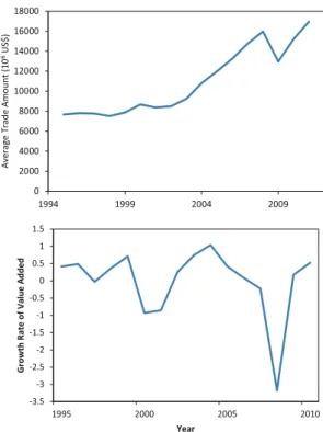
Figure 1 depicts the growth of international trade. The average amount of trade per node increased monotonically from 1995 to 2011, except for the year 2008 in which there was a financial crisis in 2008 caused by the crash of the housing bubble in the US. As a result, the interdependent relationship of the global economy has become strengthened.

The industry sector-specific international trade network is specified by nodes of industry sector α of country A and links of trade amount wAα,Bβ between industry sector α of country A and sector β of country B. The size of industry sector α of country A is measured by its value added.

Based on this basic understanding, we conducted community analysis with link identification and synchronization analysis using the World Input-Output Database.

8

(10)

0 2000 4000 6000 8000 10000 12000 14000 16000 18000

1994 1999 2004 2009

Average Trade Amount (106US$)

-3.5 -3 -2.5 -2 -1.5 -1 -0.5 0 0.5 1 1.5

1995 2000 2005 2010

Growth Rate of Value Added

Year

Figure 1: Trade and Business Cycles: (a) Amount of Import in USA and (b) Average growth rate of value added in USA

(11)

B. Global Production Data

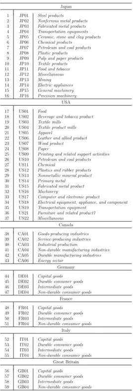
G7 Global Production Data is complied by the use of monthly time series of production index, which is open from each government of G7 countries [36, 37, 38, 39]. Duration of the data is from January1998 to January 2015 and therefore includes the global economic crisis initiated by the bankruptcy of Lehman Brothers in 2008. The items of G7 Global Production Data are listed in Table 1.

Correlation matrices were estimated for time windows of 5 year. Each time window is slided by 1 years, thus we have 13 period where correlation matrices were estimated. For instance, period 1 corresponds to the duration from 1998 to 2003 and labeled by year 2001. Similarly period 2 corresponds to the duration from 1999 to 2004 and labeled by year 2002, and so on.

IV. Results

A. Community Structure of Trade Network

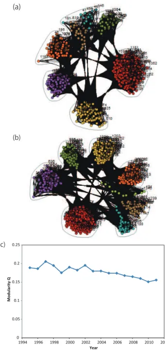
We identified the community structure for each time slice of the international trade network. Figure 8 (a) and (b) lists examples of community structures obtained for 1997 and 2009. There were 7 communities for 1997, and 8 for 2009. Because we have a few small community, the number of major community is equal to six. Temporal change of modularity Q is shown in Fig. 8 (c). The value of obtained modularity Q is about 2, which depends of threshold of the weight of links wAα,Bβ. In this community analysis we applied threshold of weight wij > 10⁷ US$. This means that about half of links are included in the analysis. If we increase the threshold of weight, we have larger value of modularity Q.

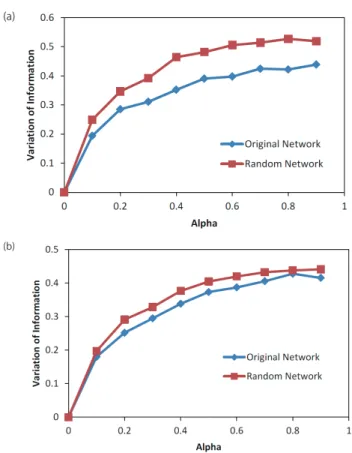
Then the robustness of identified community structure was confirmed using the variation of information V (c, c^′). The obtained results are shown in Fig. 3 for 1995 and 2011. From the value of modularity Q and the dependence of the variation of information on the probability of changing links α, we can say for a fact that the community structure is barely identified with the threshold of weight wij > 10⁷ US$.

B. Linked Communities of Trade Network

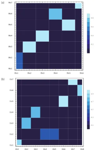
The temporal evolution of communities is characterized by the link relations for communities in adjoining years. The similarity of communities ci and cj

in adjoining years was measured by using the Jaccard index J(ci, cj). Figure 9 shows the Jaccard indices between 1995 and 1996, and the indices between

(12)

Table 1: G7 Global Production Data

Japan 1 JP01 Steel products 2 JP02 Nonferrous metal products 3 JP03 Fabricated metal products 4 JP04 Transportation equipments 5 JP05 Ceramic, stone and clay products 6 JP06 Chemical products

7 JP07 Petroleum and coal products 8 JP08 Plastic products 9 JP09 Pulp and paper products 10 JP10 Textile products 11 JP11 Food and tobacco 12 JP12 Miscellaneous

13 JP13 Mining

14 JP14 Electric appliances 15 JP15 General machinery 16 JP16 Precision machinery

USA

17 US01 Food

18 US02 Beverage and tobacco product 19 US03 Textile mills

20 US04 Textile product mills 21 US05 Apparel

22 US06 Leather and allied product 23 US07 Wood product

24 US08 Paper

25 US09 Printing and related support activities 26 US10 Petroleum and coal products 27 US11 Chemical

28 US12 Plastics and rubber products 29 US13 Nonmetallic mineral product 30 US14 Primary metal

31 US15 Fabricated metal product 32 US16 Machinery

33 US17 Computer and electronic product

34 US18 Electrical equipment, appliance, and component 35 US19 Transportation equipment

36 US21 Furniture and related product7 37 US22 Miscellaneous

Canada 38 CA01 Goods-producing industries 39 CA02 Service-producing industries 40 CA03 Industrial production

41 CA04 Non-durable manufacturing industries 42 CA05 Durable manufacturing industries 43 CA06 Energy sector

Germany 44 DE01 Capital goods 45 DE02 Durable consumer goods 46 DE03 Intermediate goods 47 DE04 Non-durable consumer goods

France 48 FR01 Capital goods 49 FR02 Durable consumer goods 50 FR03 Intermediate goods 51 FR04 Non-durable consumer goods

Italy 52 IT01 Capital goods 53 IT02 Durable consumer goods 54 IT03 Intermediate goods 55 IT04 Non-durable consumer goods

Great Britain 56 GB01 Capital goods 57 GB02 Durable consumer goods 58 GB03 Intermediate goods 59 GB04 Non-durable consumer goods

(13)

(a)

(b)

0 0.05 0.1 0.15 0.2 0.25

1994 1996 1998 2000 2002 2004 2006 2008 2010 2012

Modularity Q

Year

(c)

Figure 2: Community Analysis: (a) community structure in 1997, (b) community structure in 2009 and (b) temporal change of modularity

12

(14)

(a)

(b)

Figure 3: Variation of Information: (a) 1995 and (b) 2011

(15)

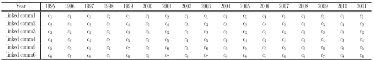
Table 2: Linked communities

Year 1995 1996 1997 1998 1999 2000 2001 2002 2003 2004 2005 2006 2007 2008 2009 2010 2011 linked comm1 c1 c1 c1 c2 c1 c1 c2 c1 c1 c1 c1 c1 c1 c1 c1 c1 c1

linked comm2 c2 c3 c2 c3 c4 c2 c4 c3 c3 c3 c2 c3 c2 c2 c3 c4 c2

2010 and 2011. Communities were arranged in decreasing order of the number of industry sectors in each community. For instance 95c1 (community c1 in 1995) is the largest, and 95c2 is the second largest. The indices for node 95c2 were displaced vertically relative to node 95c1 for better visibility. All other indices were displaced vertically in the same manner.

We define link relation for the pair of communities with the largest Jaccard index between adjoining year. We observed clearly linked relationships for most of communities. For instance, nodes 95c1 (community c1 in 1995), 95c2, 95c3, 95c4, 95c5, and 95c6 are linked to nodes 96c1 (community c₁ in 1996), 96c3, 96c4, 96c6, 96c5, and 96c7, respectively. Similarly, nodes 10c1 (community c1

in 2010), 10c4, 10c2, 10c3, 10c6, and 10c8 are linked to nodes 11c1 (community c₁ in 2011), 11c2, 11c3, 11c4, 11c5, and 11c6, respectively. We used this means to identify five linked communities between 1995 and 2011 as shown in Table 2. The identified link structure shows that a six-backbones structure exists in the international trade network.

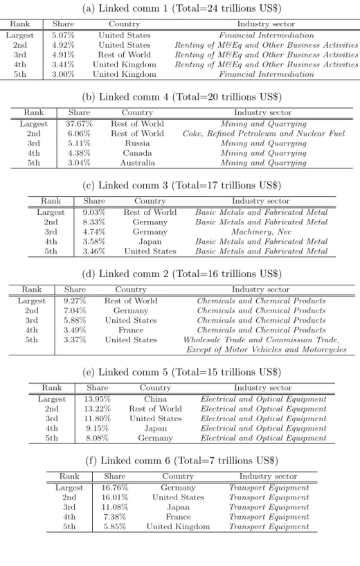
The composition of the linked communities was analyzed in terms of the marginal rank of the trade volume in countries and industry sectors. The respective compositions of the first to the fifth linked communities are listed in Table 3. Certain features of the compositions of these linked communities are briefly described below. The first linked community consists the metal and chemical materials and the electrical and transport equipment industries in primarily European countries. The second linked community and the fifth linked community contain similar industry sectors. Next, the second linked community and the fourth linked community contain similar industry sectors but different country group. The second linked community includes China and South Korea. While the fourth linked community includes the US and Canada. In addition, the third linked community consists of various countries from all over the world. The business sectors in this linked community are different from other linked communities, because the major sectors are trade and finance.

14

(16)

96c1 96c2 96c3 96c4 96c5 96c6 96c7

95c1 95c2 95c3 95c4 95c5 95c6

(a)

11c1 11c2 11c3 11c4 11c5 11c6 11c7

10c1 10c2 10c3 10c4 10c5 10c6 10c7 10c8

(b)

Figure 4: Jaccard index: (a) between 1995 and 1996, and (b) between 2010 and 2011

(17)

Table 3: Composition of Linked Communities

(a) Linked comm 1 (Total=24 trillions US$)

Rank Share Country Industry sector

Largest 5.07% United States Financial Intermediation

2nd 4.92% United States Renting of M&Eq and Other Business Activities 3rd 4.91% Rest of World Renting of M&Eq and Other Business Activities 4th 3.41% United Kingdom Renting of M&Eq and Other Business Activities 5th 3.00% United Kingdom Financial Intermediation

(b) Linked comm 4 (Total=20 trillions US$)

Largest 37.67% Rest of World Mining and Quarrying

2nd 6.06% Rest of World Coke, Refined Petroleum and Nuclear Fuel

3rd 5.11% Russia Mining and Quarrying

4th 4.38% Canada Mining and Quarrying

5th 3.04% Australia Mining and Quarrying

(c) Linked comm 3 (Total=17 trillions US$)

Largest 9.03% Rest of World Basic Metals and Fabricated Metal 2nd 8.33% Germany Basic Metals and Fabricated Metal

3rd 4.74% Germany Machinery, Nec

4th 3.58% Japan Basic Metals and Fabricated Metal 5th 3.46% United States Basic Metals and Fabricated Metal

(d) Linked comm 2 (Total=16 trillions US$)

Largest 9.27% Rest of World Chemicals and Chemical Products 2nd 7.04% Germany Chemicals and Chemical Products 3rd 5.88% United States Chemicals and Chemical Products 4th 3.49% France Chemicals and Chemical Products 5th 3.37% United States Wholesale Trade and Commission Trade,

Except of Motor Vehicles and Motorcycles

(e) Linked comm 5 (Total=15 trillions US$)

Largest 13.95% China Electrical and Optical Equipment 2nd 13.22% Rest of World Electrical and Optical Equipment 3rd 11.80% United States Electrical and Optical Equipment 4th 9.15% Japan Electrical and Optical Equipment 5th 8.08% Germany Electrical and Optical Equipment

(f) Linked comm 6 (Total=7 trillions US$)

Largest 16.76% Germany Transport Equipment 2nd 16.01% United States Transport Equipment

3rd 11.08% Japan Transport Equipment

4th 7.38% France Transport Equipment

5th 5.85% United Kingdom Transport Equipment

16

(18)

C. Synchronization of International Business Cycles

The phase time series θj(t)(j = 1, · · · , 1435) for the growth rate of value added were evaluated for the years 1995 to 2011 using the methodology described in subsection a.

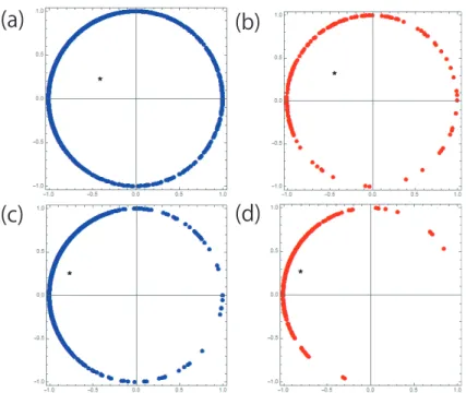
Figure 5 shows the polar plot of phase in 1997 for (a) all sectors, (b) community c1, (c) community c2, and (d) community c3. In these polar plots, the complex order parameter u(t) is indicated by a black asterisk. The respective amplitude for the order parameters are 0.483, 0.359, and 0.534 for community c1, c2, c3, respectively. While the amplitude for all sectors is 0.253. The respective amplitude for the order parameter of each community was observed to be greater than the amplitude for all sectors. This means that active trade produces higher phase coherence within each community.

Figure 5 shows the polar plot of phase in 2009 are shown in for (a) all sectors, (b) community c1, (c) community c2, and (d) community c3. In these polar plots, the complex order parameter u(t) is indicated by a black asterisk. The respective amplitude of the order parameters are 0.758, 0.512, 0.801 for community c1, c2, and c3, respectively. While the amplitude for all sectors is 0.662. Amplitude r(t) and average phase φ(t) for each community is equiva- lent to those quantities for all sectors. The respective amplitude for the order parameter of each community was observed again to be greater than the amplitude for all sectors. It was noted that the amplitudes and average phases in 2009 are larger than the quantities in 1997. This relation clearly indicates that interdependent relationship of the global economy has become stronger.

Figure 6 shows the temporal change in amplitude for the order parameter r(t) for the years 1996 to 2011. Phase coherence decreased gradually in the late 90’s but increased sharply in 2001 and 2002. This temporal change might be related to the structural change in the international trade network discussed in subsection A. From 2002, the amplitudes for the order parameter r(t) remain high except for the years 2005 and 2009. The decrease in 2009 was caused by financial crisis resulting from the housing bubble crash in the US but the cause of the decrease in 2005 is unclear.

Order parameters are estimated for the growth rate of the value added time series shuffled randomly with keeping auto-correlation [20, 21] and order parameter averaged over 1000 shuffled time series is plotted by black curve. This means that average order parameter is evidently larger than the systematic error of the analysis method. Therefore the synchronization observed for each linked communities is statistically significant. Thus it should be noted that existence of the synchronization in the international trade network is fully- clarified.

(19)

(a) _(b)

(c) (d)

Figure 5: Polar plot of phase for growth rate of value added: (a) all communities in 1997, (b) community c1 in 1997, (c) all communities in 2009, and (d) community c1 in 2009

0 0.1 0.2 0.3 0.4 0.5 0.6 0.7 0.8 0.9 1

Order Parameter

all sector linked comm1 linked comm2 linked comm3 linked comm4 linked comm5 linked comm6

Figure 6: Temporal change of amplitude for the order parameter r(t)

18

(20)

1998 2000 2002 2004 2006 2008 2010 2012 2014 0

5 10 15 20

1998 2000 2002 2004 2006 2008 2010 2012 2014

Year

λ

Eigenvalues

1998 2000 2002 2004 2006 2008 2010 2012 2014

0 1 2 3 4

5 ¹⁹⁹⁸ ²⁰⁰⁰ ²⁰⁰² ²⁰⁰⁴ ²⁰⁰⁶ ²⁰⁰⁸ ²⁰¹⁰ ²⁰¹² ²⁰¹⁴

0 1 2 3 4 5

Year

#

Number of Significant Modes

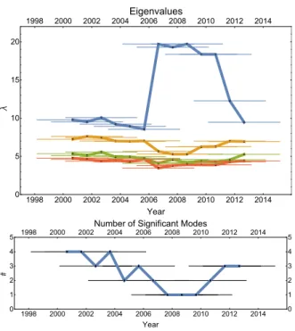
Figure 7: Eigenvalues of Significant Modes

D. Significant Modes in Economic Crisis

In the analysis of G7 Global Production Data, we obtained eigenvalues for the correlation matrix C from Eq.(18) and selected statistically significant modes using the rotational random shuffling. In the rotational random shuffling, the growth rate of production time series x(t) was shuffled randomly with keeping autocorrelation [20, 21] and then eigenvalues for the correlation matrix were calculated for the randomly shuffled time series. If an eigenvalue for the original time series is larger than the largest eigenvalue calculated for the randomly shuffled time series, the eigenvalue or eigen mode is regarded as statistically significant. The largest four eigenvalues of each period are shown in the upper panel of Fig. 7. The lower panel depicts temporal change of the number of significant modes. Note that only a single eigen mode is significant for the periods that contain the sub prime mortgage crisis of 2008. This means that production for all industry sectors in G7 countries behaves similarly during economic crisis. The economic risk propagate instantaneously to All industry sectors in G7 countries and all industries decrease their production simultaneously.

(21)

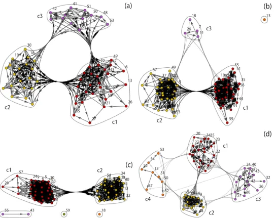
E. Community Structure of Production Network

We identified the community structure for each time slice of the global production network constructed using the methodology described in section c. Figure 8 shows examples of community structures obtained for (a) 2004, (b) 2007, (c) 2010, and (d) 2013. Average value of modularity Qs is 0.302 during 2001 and 2013. Maximum and minimum of modularity are 0.410 and 0.153, respectively. The means that the community structure is clearly identified for the global production network. The number of major communities varies between two and four. There were two major communities for the global economic crisis during 2007 and 2010. The observed community structure is consistent to the statistically significant modes obtained above. The number of major community in the period of normal economy (2004 and 2013) is larger than the period of economic crisis (2007 and 2010). The small number of statistically significant mode in economic crisis is observed as the small number of major communities in the global production network. This is interpreted again such that production for all industry sectors in G7 countries behaves similarly during economic crisis. The economic risk propagate instantaneously to All industry sectors in G7 countries and all industries look for new demand. Consequently new links (trade relations) are spanned beyond communities observed in the period of normal economy.

F. Linked Communities of Production Network

The temporal evolution of communities is characterized by the link relations for communities in adjoining years. The similarity of communities ci and cj in adjoining years was measured by the use of the Jaccard index J(ci, cj). Figure 9 shows the Jaccard indices in adjoining years: (a) between 2003 and 2004, (b) between 2006 and 2007, (c) between 2009 and 2010, and (d) between 2012 and 2013. Communities were arranged in decreasing order of the number of industry sectors in each community. For instance community c1 is the largest, and c2 is the second largest.

We define link relation for the pair of communities with the largest Jac- card index between adjoining year. Most of communities show clearly linked relationships with communities of the adjoining year. For instance, Fig. 9 (a) shows that communities c1, c2, c3, and c4 in 2003 are linked to communities c2, c1, c1, and c3 in 2004, respectively. Similarly, Fig. 9 (c) shows that communities c1 and c2 in 2009 are linked to communities c1 and c2 in 2010, respectively. The obtained linked communities are summarized in Table 4, LinkedComm2, and LinkedComm3 for three periods: before the crisis, during the crisis, after

20

(22)

1 3 4

5

6

7

9

10 11 12

13

14 15

16 17

19 18

20

21 23 22

24 1

1 1777777777²⁵

26

27 28

29 30

31 32

33

35 36

37

38

39 ⁴⁰

41 42

43 44

45 46

47 48

4 4 49 50 51

52 53

54

55 56

57 58

59

(a)

c1 c2

c3

1 2 3 5 6

7

9 8

10 11

12

13

15 14 16 18

19 20 21

22 23

24 25

26

2 28

9 30

31 32

33

34 ₃₅

36 37

38 39

41 40 43

44 45 46 47

4 49

50

51 52

53 54

55

56 57

58

59

(b)

c1 c2

c3

1 2

3 5

6

8 9

10

11 1

13 4

15

16

18 2219

3

24 2

26

2 8 30

1

32 33

34 35

36 3

38

39

40

41 2

43

44 45 46

47

48 49

50 51 53 52

54

55

56 57

58

59

c1 c2 (c)

1

2 ⁴

6 5

2⁸ 9

1 11

12 13

14 16 1817

19 20

21 22 23

24 25

26 27

2 2

30 31

3 32 3435

36 37

38

39 3

40

42 43 44

45 46

47

48

49 50

51

52 53

54 55

56

57 58

59

(d)

c1

c2 c4 c3

(23)

Table 4: Linked communities before the crisis

Year 2001 2002 2003 2004 2005 2006

Linked comm 1 c₁ c₂ c₂+ c₃ c₁ c₂ c₃

Linked comm 2 c₂ c₁ c₁ c₂ c₁ c₂

Linked comm 3 c3+ c4 c3 c4 c3 c3 c1

Table 5: Linked communities during the crisis

Year 2008 2009 2010

Linked comm 4 c2 c1 c1

Linked comm 5 c₁ c₂ c₂

Table 6: Linked communities after the crisis

Year 2012 2013

Linked comm 6 c₁ c₃ Linked comm 7 c₂ c₁ Linked comm 8 c3 c2

Linked comm 9 c₄ c₄

the crisis, respectively. The temporal change of communities structurer, i.e. community dynamics is regarded as an example of collective motion.

We obtained three linked communities before the crisis. Linked communities 1 to 3 are characterized by countries and corresponds to Europe, US, Canada, respectively. Japan distributed to three communities.

Then two Linked communities (linked communities 4 and 5) were obtained for the period of the crisis. Linked communities 4 and 5 are characterized by sectors. For instance, linked community 4 is composed by sectors: Steel products, Transportation equipments, Chemical products, Pulp and paper products, Computer and electronic product, and others. Linked community 5 is composed by sectors: Fabricated metal products, Precision machinery, Textile products, and others.

We obtained four linked communities after the crisis. Linked communities 6 to 9 are characterized by countries as before. For instance, linked communities 6 to 9 corresponds to Canada, US, Japan, and Europe. Some European countries distributes to linked communities 6 and 7.

G. Communities in Multiplex Production Network

The dynamics of community structure is observed in the temporal change of community structure for the 13 layer multiplex network. We used parameter rs = 1, inter slice coupling Cisr = 0.8. Color of each node corresponds to

22

(24)

0.1 0.2 0.3 0.4 0.5 0.6

c1 c2 c3 c4

Communities in 2003 c1

c2 c3

Communities in 2004

(a)

0.1 0.2 0.3 0.4

c1 c2 c3 c4

c2

Communities in 2007