博士論文、修士論文

(1)

Gamma-ray and X-ray Study of Relativistic Jets in

Gamma-ray Burst Sources detected with

Swift

Goro Sato

Reproduced from the thesis submitted to

the University of Tokyo for

the Degree of Doctor of Philosophy (Physics)

(2)

Abstract

Gamma-ray bursts (GRBs) are the most powerful explosions in the universe, which take place at the cosmological distances. The Swift mission, launched on November 20, 2004, is the first mission with ability to begin multi-wavelength observations within_∼1 minute after the detection of GRBs. Swiftmonitors a large field of view (FOV) with the gamma-ray imager and, if identifies a GRB, quickly slews to point two narrow FOV telescopes (X-ray and UV/optical) on the same spacecraft to the GRB position. We participated the development of the key instrument, Burst Alert Telescope (BAT) and developed the energy response function which is used to determine the gamma-ray spectra.

BAT detected 77 GRBs and conducted early follow-up observations from 50–350 sec in 46 cases before September 2005. It is reported by theSwiftteam that there is a possible canonical behavior in X-ray afterglow starting with a rapid decay (tα_;_{α <}₋_{3), followed}

by a shallow decay (α _{∼ −}0.5), and then somewhat steeper decay (α _{∼ −}1.2). X-ray flares are additionally observed in case. Analyzing X-ray data of GRB 050319 and GRB 050713, we confirm the features of rapid decay and X-ray flares.

Since jet breaks are explained as being due to a hydrodynamical transition of the jet, the break is wave-length independent, and therefore should be observable in X-rays. Once jet break time is obtained, one can calculate the jet opening angle and hence collimation corrected “true” burst energy (Eγ). It is known that there is a tight correlation between

the spectral peak energy (Esrc

peak) and Eγ(Ghirlanda relation; Epeaksrc ∝Eγ0.7). However, no

clear evidence for jet breaks is obtained except for a few cases.

To investigate this mysterious situation, we select and study GRB 050401, XRF 050416a, and GRB 050525a with redshift determinations, well characterized prompt emis-sions and well sampled X-ray afterglows. We first find that the bursts satisfy the Amati relation between Esrc

peakand the burst energy before collimation correction (Epeaksrc ∝Eiso0.5),

which is consistent with the prediction of the standard synchrotron shock model. Next, we investigate jet break features in their X-ray lightcurves. However, none of the seg-ments is consistent with the relation between the spectral and temporal indices predicted for the phase after jet break. We therefore use the Ghirlanda relation inversely to predict the jet break time. However, there are no temporal breaks within the predicted time intervals.

(3)

List of Figures

2.1 All sky map of 2704 gamma-ray bursts detected with BATSE instrument

during the nine-year mission. . . 4

2.2 Images of the fading X-ray afteglow of GRB 970228 detected by BeppoSAX satellite. . . 5

2.3 Hubble image of the optical afterglow of GRB 970228. . . 6

2.4 Redshift distribution before the Swift era. . . 6

2.5 The light curves of GRBs detected by BATSE . . . 7

2.6 Distribution of the burst duration and a scatter plot between the duration and spectral hardness of the 4B Catalog GRBs recorded with BATSE. . . 8

2.7 TheνFν spectra of GRB 91601, 920622, 910814 observed by CGRO multi-instruments. . . 9

2.8 The correlation between the isotropic equivalent energyEiso and the spec-tral peak energy in the source frame Esrc peak. . . 10

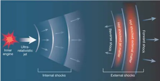
2.9 Drawing of the internal-external shock scenario. . . 12

2.10 The expected synchrotron spectra and light curves. . . 14

2.11 Illustration of the expansion of a collimated shell. . . 16

2.12 The optical and radio light curves of GRB 990510, showing a jet break feature. . . 17

2.13 The distribution of the apparent isotropic gamma-ray energy and the ge-ometry corrected energy. . . 18

2.14 The peak energy in the source frame Esrc peak against the burst energy before and after collimation corrected. . . 19

3.1 The Swift satellite. . . 21

3.2 The drawing of Burst Alert Telescope on-board the Swift spacecraft. . . . 23

3.3 The BAT Detector Module (DM). . . 25

3.4 The coded aperture mask. . . 26

3.5 The response of the BAT to a simulated GRB. . . 27

(7)

3.8 Simulated spectrum from 100 s XRT observation of a typical 150 mcrab after glow at z = 1.0, assuming a powerlaw spectrum plus a Gaussian Fe

line at 6.4 keV. . . 31

4.1 A typical 57_{Co spectrum obtained with a single CdZnTe detector. . . . .} ₃₄

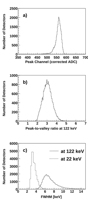
4.2 Distributions of spectral parameters for 32K CdZnTe detectors. . . 35

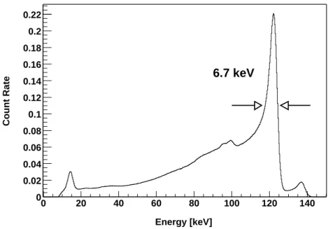
4.3 Summed spectrum of 32K CdZnTe detectors for 57_{Co. . . .} ₃₆

4.4 The “depth distribution” for 122 and 136 keV lines. . . 38

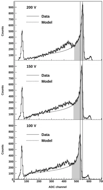
4.5 The 57_{Co spectra taken at three different bias voltages. . . .} ₄₀

4.6 A cross-plot of µτ for electrons and µτ for holes. . . 41

4.7 Spectra obtained with single CdZnTe detectors with various sets of µτ products. . . 42

4.8 The µτ products cross-plot showing corresponding peak-to-valley ratio. . 43

4.9 The extracted µτ products against detector number sorted by ingot ID . 44 4.10 The distributions of µτ for electrons and µτ for holes at three different temperatures. . . 45

4.11 The measured temperature dependence of µτ products. . . 45

4.12 An 241_{Am spectrum obtained with a single CdZnTe detector. . . .} ₄₆

4.13 A 109_{Cd spectrum obtained with a single CdZnTe detector. . . .} ₄₇

4.14 The “depth distributions” at three different angles and the spectral models produced from the distributions. . . 48

4.15 The “depth distributions” for K-escapes for a stream of 122 keV photons and the spectral model produced from the distributions. . . 49

4.16 Theµτ products cross-plot divided into 9-by-7 groups with equal intervals in log-scale. . . 50

4.17 A 57Co summed spectrum fitted with the composite spectral model. . . . 50

4.18 A 133_{Ba summed spectrum fitted with the composite spectral model.} _{. .} ₅₁

4.19 Two dimensional image of the BAT detector response matrix. . . 52

4.20 On-board calibration spectrum of the 241_Am_{source. . . .} ₅₃

4.21 Fit to the Crab using the corrected response matrix, and including the systematic error vector. . . 54

5.1 The GRB detection history of Swift BAT instrument from the first detec-tion on December 17, 2004 to the end of September 2005. . . 57

5.2 The BAT effective area with and without taking into account the coded aperture mask. . . 59

5.3 The light curve of GRB 050716 in 15-150 keV before and after the back-ground subtraction with the mask-weight technique. . . 60

(8)

5.6 The Swift BAT spectrum of GRB 050716 fitted with the Band function. 62

5.7 Distribution of the burst duration T90 for the 77 Swift GRBs. . . 63

5.8 The hardness ratio of flux in 50–150 keV over that in 15–50 keV is plotted against the burst duration T90. . . 64

5.9 Distribution of photon index obatained by the fit with a single power law model. . . 65

5.10 The fluence in 15–150 keV against the burst duration T90. . . 66

5.11 F-test probability of an improvement in χ2 _{fit of simulated spectra from} the single power law model to the cut-off power law model. . . 67

5.12 Photon index obtained from the simulated spectra fitted with a power law model. . . 67

5.13 The distribution of the Swift XRT observation start time with the com-parison to the X-ray observations conducted in the pre-Swift era. . . 70

5.14 Canonical behavior of X-ray afterglows. . . 71

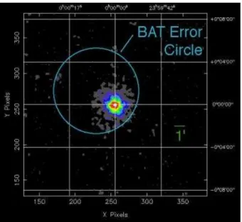
5.15 X-ray image of the GRB 050319 afterglow. . . 72

5.16 The event distributions around the GRB centroid. . . 73

5.17 X-ray light curve of GRB 050319 in 2–10 keV. . . 74

5.18 X-ray image of the GRB 050713a afterglow. . . 75

5.19 X-ray light curve of GRB 050713a in 2–10 keV. . . 76

6.1 The distribution of jet break time observed in the previous GRBs. . . 78

6.2 The νFν spectrum of GRB 050401 observed with Konus-Wind. . . 81

6.3 X-ray afterglow light curve of GRB 050401 in 2–10 keV. . . 82

6.4 The νFν spectrum of XRF 050416a observed withSwift BAT. . . 83

6.5 X-ray afterglow light curve of XRF 050416a in 2–10 keV. . . 84

6.6 The νFν spectrum of GRB 050525a observed with Swift BAT. . . 85

6.7 X-ray afterglow light curve of GRB 050525a in 2–10 keV. . . 86

6.8 The relation between the rest-frame peak energy Esrc peak and the isotropic equivalent energy, Eiso. . . 90

6.9 The temporal indexαas a function of the spectral index βof the observed X-ray afterglows. . . 91

6.10 The rest-frame Esrc peak as a function of the collimation-corrected energy Eγ. 95 A.1 The light curves of Swift GRBs which are categorized to short GRBs. . 98

A.2 The light curves of Swift GRBs shown between ₋100 and +100 s from the BAT triggers. The background is subtracted with mask-weighting technique. . . 99

A.3 Continued. . . 100

(9)

A.7 Continued. . . 104 A.8 Continued. . . 105 A.9 The light curves of Swift GRBs which have relatively long duration. The

light curves are shown between₋300 and +300 s from the BAT triggers. 106 A.10 Continued . . . 107

B.1 The Swift Mass Model, containing most of all the components in the space-craft. The coded aperture mask is not drawn in this figure to show the CdZnTe detector array. . . 109 B.2 The light curve of GRB 041223 before the background subtraction. The

foreground and background time interval used in the SwiMM analysis is shown. . . 110 B.3 The joint spectral analysis of GRB 041223 using mask weight technique

and SwiMM. The data indicated byblackandredare the spectra extracted by the mask weight method and that extracted by the time domain back-ground subtraction method. . . 110 B.4 The same spectra with Fig. B.3in νFν representation. The fit extended

to 350 keV in conjunction with the SwiMM Monte Carlo method provides better finding ofEobs

peak. . . 111

(10)

List of Tables

3.1 BAT Instrument Paramters. . . 24

3.2 XRT Instrument Properties. . . 29

4.1 Required detector performance specifications. Peak-to-valley ratio at 14.4 keV is defined as Peak14/LValley where Peak14= average counts from 3 channels around 14.4 keV and LValley = average counts from 3 channels in the valley between the 14.4 keV peak and the lower energy threshold. Peak-to-valley ratio at 122 keV is defined as Peak122/Peak100 where Peak122 and Peak100 are averages counts from 3 channels around 122 and 100 keV, respectively. 33 5.1 The spectral parameters of GRB 050716 obtained with the power law, the cut-off power law, and the Band function. . . 62

5.2 Characteristics of the 77 Swift GRBs. . . 68

5.2 Characteristics of the 77 Swift GRBs. . . 69

6.1 GRB Sample Parameters . . . 79

(11)

Chapter 1 Introduction

Gamma-ray bursts (GRBs) are brief flashes with enormous amount of gamma-rays which occur at unpredictable locations in the sky. The origin of the phenomena has long been in a deep mystery since its discovery in 1967. Because of the recent observational and theoretical advances especially in 1990’s and later, it is found that the gamma-rays are coming from cosmological distances as far as 10 billion light years away, and therefore it is revealed that the gamma-rays are sparks of the most powerful explosions in our universe since Big Bang. The emitted energy amounts from 1051_{to 10}54_{erg if an isotropic emission}

is assumed. This is comparable to the energy converting a solar mass entirely in a few seconds ( _∼ 2_×1054 _{erg). Probably such a huge amount of energy is available only in}

a core collapse of a very massive star, or merging of two compact objects (Neutron Star – Neutron Star or Neutron Star – Black Hole). In either case it is believed that the phenomenon is related to a birth or a growth of Black Hole.

In current understanding, GRB originates from a jet-like collimated outflow with a bulk Lorentz factor of Γ >100, which is the most relativistic object we know. However neither the mechanism of jet formation nor physical processes in the accelerated matters are well understood. The gamma-ray bursts are therefore one of the most interesting and important astronomical objects and have an unique capability to shed light on physical processes in such extreme situations. Recently, it is also anticipated to utilize the enor-mous luminosity of GRBs as a probe of early universe, which may lead to, e.g., constraint of the cosmological parameters.

The Swift mission (Gehrels et al. 2004), launched on November 20, 2004, is a multi-wavelength observatory dedicated for GRB astronomy. It is a first-of-its-kind autonomous slewing satellite for transient astronomy and pioneers the way for future rapid-reaction and multi-wavelength missions. It is far more powerful than any previous GRB mission, observing more than 100 bursts per year and performing detailed X-ray and UV/optical afterglow observations spanning timescales from 1 minute to several months after the burst.

(12)

4 arcmin accuracy. Since a large filed of view is indispensable to localize a large number of GRBs as well as the precise angular resolution, the BAT utilizes a coded aperture tech-nique. There are 32,768 pieces of CdZnTe (4_×4 mm2_{, 2 mm thick) to form a 1}_.₂_×₀_.₆

m2 _{sensitive area in the detector plane. CdZnTe is employed because of its attractive}

merits of a high quantum efficiency for gamma-rays and its capability of to fabricate such a large array with small pixel size. However, the charge loss of considerable amount in CdZnTe detectors distorts a resultant gamma-ray spectrum. In order to study a spectral property of GRBs, a correct understanding of the detector energy response is of great importance. We have developed our original method to measure charge transport prop-erties in CdZnTe at ISAS/JAXA. Three and half years before the launch, we started to participate the BAT calibration test performed at NASA/GSFC and carried out charac-terization of all the CdZnTe detectors with our method. The development of detector response function of the BAT are our most significant contribution to the Swiftmission. Since the launch of Swift satellite, Swift has conducted about 20,000 successful slews to targets and Swift BAT has continuously observed new gamma-ray bursts at a rate of 100 per year. All of Swift 77 GRBs as of the end of September 2005 are systemat-ically analyzed and discussed in this thesis. We review on the recent understanding of observational and theoretical approach in Chap. 2. The basic feature and performance of Swift satellite are summarized in Chap. 3. Our evaluation method of CdZnTe applied to BAT calibration and the detector response generation are described in Chap. 4. In Chap. 5, we list theSwiftGRB data and our systematic analysis of X-ray Telescope (XRT) and BAT observations. Temporal and spectral property in gamma-ray data of all samples are characterized and some canonical behavior of early X-ray afterglows are discussed. Chap. 6 is devoted to discuss jet break evidence with the synchrotron shock model, where we investigate the correlation of collimation-corrected energy (Eγ) with the peak energy

of the source frame (Esrc

peak) and the possibility of jet break appearance within Swift’s

(13)

Chapter 2 The Gamma-ray Bursts

2.1 Observational History of GRBs

There was a series of U.S. vela satellites from 1960’s to 1970’s. The program was run jointly by the Advanced Research Projects of the U.S. Department of Defense and the U.S. Atomic Energy Commission, managed by the U.S. Air Force. Although their primary task was looking for violations of the Nuclear Test Ban Treaty during the Cold War, they provided much useful astronomical data. On July 2, 1967, a large increase of gamma-ray emission was detected by their CsI scintillation detectors. Timing the burst arrival times between different satellites, Vela 4A, B and 3, suggested that the gamma-rays came not from the vicinity of Earth but from a region of outer space (Klebesadel, Strong & Olson 1973). This is the first detection of the gamma-ray burst recorded in history. The later four satellites (5A, B and 6A, B) recorded 73 gamma-ray bursts in the ten year interval July 1969 – April 1979. The distribution on the sky appeared to come from all directions, unlike Galactic objects which cluster near the plane or center of the Galaxy. It suggested possible three cases: they were faint and close (within a few hundred light years); they were associated with the halo of the galaxy; they were bright and very far away. Over 100 hypotheses for the origin had been suggested by 1992 such as asteroids or comets falling onto neutron stars, neutron starquakes, neutron star nova, stellar flares, black holes, white holes, active galactic nuclei, collisions of cosmic string, strange matter, supernovae and etc. (Nemiroff 1994).

(14)

Figure 2.1: All sky map of 2704 gamma-ray bursts detected with BATSE instrument during the nine-year mission, showing their isotropic distribution in the sky. The burst locations are color-coded based on the fluence, which is the energy flux of the burst integrated over the total duration of the event. From http://www.batse.msfc.nasa.gov/batse/grb/skymap/.

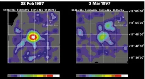
On February 28, 1997, there was a breakthrough to solve the GRB distance mystery. The Beppo-SAX satellite detected a historical gamma-ray burst, GRB 970228 with its Wide Field Camera (WFC). The WFC had a wide filed of view (FOV) of 20 degrees_×20 degrees as well as a precise localization with_∼5 arcmin accuracy. It allowed the satellite to point the X-ray telescopes onboard the same satellite _∼ 8 hours later, discovering a fading X-ray source – an X-ray afterglow, as shown in Fig. 2.2 (Costa et al. 1997). The rapid localization also enabled a multi-wavelength observational campaign which allowed the discovery of an optical afterglow and a host galaxy, e.g. HST observation shown in Fig. 2.3, leading to the discovery that the redshift of GRB 970228 is 0.695. Thus, it is finally revealed that GRBs are cosmological sources (van Paradijs et al. 1997). Before the Swift era, redshifts are determined well for 39 GRBs. Fig. 2.4 shows the redshift distribution, where the average is _∼1.3 with the highest of 4.5.

(15)

Figure 2.2: Images of the fading X-ray afteglow of GRB 970228 detected by BeppoSAX satellite. From Costa et al. (1997).

(16)

Figure 2.3: Hubble image of the optical afterglow of GRB 970228, discrim-inating a surrounding nebulosity (at 25th magnitude) which is considered a host galaxy. The right panel is the enlargement of the central region of the left panel. Black and white images indicate the locations of the GRB source and the extended emission from the host galaxy. (Fruchter, A., & NASA) From http://hubblesite.org/.

redshift

0 1 2 3 4 5 6 7

Number of Bursts

0 2 4 6 8 10 12

1997-2004

(17)

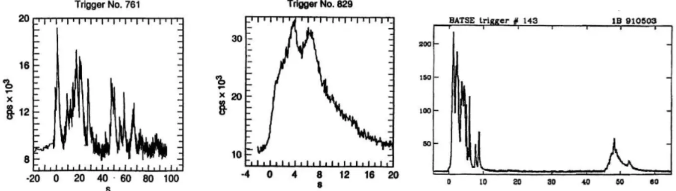
Figure 2.5: The light curves of GRBs detected by BATSE, showing a large diversity. From Fishman & Meegan (1995).

2.2 Temporal Characteristics

Let us review and summarize the properties of gamma-ray emissions observed in the BATSE gamma-ray bursts (Fishman et al. 1994; Fishman & Meegan 1995). A unique feature of gamma-ray bursts is the diversity of their light curves. Some are erratic, spiky, while some others are smooth with one or a few components. The light curves are very irregular indeed. The burst shown in Fig. 2.5 (left) has a light curve with complex temporal structures from the BATSE samples, while the burst shown in Fig. 2.5 (center) is a strong burst that shows no structures on fine time scales. On the other hand, the burst shown in Fig. 2.5 (right) has distinct, well-separated episodes of emission. Widths of inidividual pulses (δt) vary in a wide range (the shortest: sub millisecond). Most individual pulses are asymmetric, with sharper leading edges than trailing edges. The duration of gamma-ray burst is usually denoted asT90, which is the time interval during

which 90% of the burst energy is released. Fig. 2.6 (left) shows the distribution of the

T90observed by BATSE. They distributes in a rather wide range from ∼10−2 to ∼1000

(18)

BATSE SAX

0.01 0.1 1 10 100 1000 0.1

1 10 100

90% Width

S

100-300 keV

50-100keV

/ S

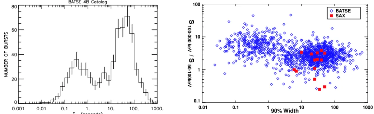
Figure 2.6: left) The distribution of the burst duration of the 4B Catalog GRBs recorded with BATSE.

From http://www.batse.msfc.nasa.gov/batse/grb/duration/.

right) Distribution of T90 duration vs. spectral hardness for BATSE bursts

(diamonds) from the 4B catalogue. Events localized by BeppoSAX (solid squares) appear to belong to the long duration class. From Kulkarni et al. (2000).

2.3 Spectral Characteristics

Another feature of gamma-ray burst is their high energy emission. The spectrum is continuum usually with a νFν peak at a few hundreds keV. Fig. 2.7 shows typical νFν

spectra of gamma-ray bustrs observed with CGRO multi-instrument. The spectrum can be phenomenologically characterized with smoothly-joint broken power law function, known as GRB function or Band function (Band et al. 1993):

N(E) =N0

  

 

EαBexp(−E

E0) , E <(αB−βB)E0 ,

[(αB−βB)E0]αB

−βB

exp(βB−αB)EβB, E ≥(αB−βB)E0 ,

(2.1)

where νF(ν) peaks at Eobs

peak = E2N(E) = (αB + 2)E0 . The function has a photon

index of αB for the lower energy part, and flattening out smoothly to a high energy tail

described with a photon index of βB. The values for αB, βB, E0 all vary between bursts,

and some time evolutions have been reported even within a single burst.

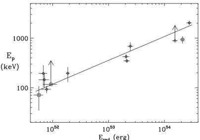
Amati et al. (2002) studied the spectral and energetics properties of BeppoSAX GRBs with redshift determinations. They investigated the time-integrated spectrum using the Band function, and found a positive correlation between the total energy and the peak energy in the source frame. The total energy is calculated in 1-10,000 keV assuming an isotropic radiation, which is defined asEiso. The peak energy is corrected for the redshift

z byEsrc

peak ≡(1 +z)Epeakobs . They found that more luminous GRBs are characterized also

by larger peak energies: Esrc

peak ∝E0.52

±0.06

(19)

Figure 2.7: The νFν spectra of GRB 91601, 920622, 910814 observed by

CGRO multi-instruments, and the best fit spectral models. From Tavani (1996).

2.4 Cosmological Fireball Model

What are GRBs? In this section, we follow the discussions which led to the development of the standard cosmological GRB model, which is well described in e.g. Piran (1999). Let us start from tracing the enormous amount of gamma-ray photons back to the GRB emitting site. The size of the emitting region can be estimated by the pulse width of the light curve (Rybicki & Lightman 1979). Since the pulse as short as δt = 10 ms is detected in the GRB emissions, the emitting region is very compact with the size,

R _≃ δt_×c

≃ 3_×108

µ

δt

10 ms

¶

cm

= 3000

µ

δt

10 ms

¶

km. (2.2)

The luminosity is also calculated from the observed energy flux F:

L = 4πd2F

≃ 1050

µ

d

3 Gpc

¶2µ

F

10−7 _{erg cm}−2

¶

(20)

Figure 2.8: The correlation between the isotropic equivalent energy Eiso

(la-beled byErad) and the spectral peak energy in the source frameEpeaksrc (labeled

byEp). From Amati et al. (2002).

where dis a distance between the source and the observer. Then, the number density of gamma-rays nγ is given as follows:

nγ =

L

4πR2_²c

≃ 2_×1027

µ

d

3 Gpc

¶2µ

F

10−7 _{erg cm}−2

¶ µ

δt

10 ms

¶−2

cm−3, (2.4)

where ² is a typical energy of the gamma-ray photons. Here we assumed ² _∼ 1 MeV. What if there is a sudden release of a large quantity of gamma-ray photons into a compact region? The electron-positron pair production γ γ _−→ e+_e− _{occurs if} √_E

1E2 > mec2,

where E1 and E2 are energy of interacting photons. The optical depth τγγ along the

region size R is obtained as

τγγ = σTnγR

≃ 4_×1011

µ

d

3 Gpc

¶2µ

F

10−7 _{erg cm}−2

¶ µ

δt

10 ms

¶−1

, (2.5)

whereσT is the Thomson cross-section. We can realize an emerge of the opaque

photon-lepton “fireball”. However, since gamma-rays cannot survive in the fireball, the radiation cannot escape. This is known as the “compactness problem”.

(21)

θ is affected by a factor ofδ = 1/Γ(1₋βcosθ), which is called “beaming effect” (Rybicki & Lightman 1979). When the angle cosθ _∼ β, the photon is blue-shifted by δ _∼Γ, and hence the energy can be lower than the sufficient energy for pair production. According to the detailed calculation, the cross-section becomes lower by a factor of Γ−2α _assuming

a power law distribution with the high-energy spectral index of α. In addition, when the emitting region moves toward the observer, the observed time scale is shorter by a factor of 1/2Γ2_{. The emitting region therefore can be larger by the same factor. Thus,}

the optical depth can be decreased by the relativistic motion as follows:

τγγ ∝ Γ−2α−2. (2.6)

The spectral indexαis typically from 2 to 3. In order to obtain an optically thin fireball, it requires approximately Γ_≥100.

This relativistic motion can be understood as a natural attribute of the time evolution of a pure radiation fireball. Because of the opacity of pair production, the fireball becomes photon-lepton plasma, which behaves like a perfect fluid. The local temperature drops with T _∝ R−1 _{with a free expansion, where} _R _{is a radius. Energy conservation requires}

EΓ = const., and hence Γ _∝ E−1 _∝ _T−1 _∝ _R_{. Thus the fireball is accelerated and}

expanding relativistically outwards. After the temperature drops low enough that pair annihilation dominates, gamma-rays can escape from the region and become detectable by the observer. However, the spectrum thus obtained is thermal with the temperatureTΓ, which is equal to the initial temperature. This difficulty is solved by a contamination of baryonic matters. The baryonic load increases the opacity even after τγγ becomes

negligible, and convert the part of received energy into the bulk kinetic energy. As a result, the matter coast asymptotically with a constant Lorentz factor. The baryonic mass is required being as small as _∼ 10−6_M

¯ so that the fireball becomes relativistic,

otherwise the fireball cannot be accelerated enough and becomes Newtonian.

2.5 The Internal-External Shock Scenario

The energy carried by the matter-dominated outflow should be somehow converted into radiation again to produce the gamma-ray burst emissions. The shock dissipation is most likely mechanism to provide such energy transfers. Fig. 2.9 illustrates the standard GRB fireball model. Let us assume a several or tens of blobs are ejected from the central engine of the gamma-ray burst. Due to Lorentz contractions, each blob looks like a thin “shell” for the observer in the rest frame. Collisions take place between the shells with different velocities. The collision distance is estimated as _∼ 1014 _{cm. This is called “internal}

(22)

Figure 2.9: Drawing of the internal-external shock scenario. From Piran (2003).

show more smooth changes, which is the afterglow. This is called “external shock”.

2.5.1 Internal Shock

Here, we follow the calculations in Kobayashi, Piran & Sari (1997). We assume that a relatively slow shell with the mass of Ms and the Lorentz factor of Γs is ejected, and then

another relatively rapid shell withMr and Γr is ejected. The rapid shell can catch up the

slow one, and two merge to form a single one. Energy and momentum conservation gives a bulk Lorentz factor of merged shell as:

Γm ≃

s

MrΓr+MsΓs

Mr/Γr+Ms/Γs

. (2.7)

The difference of the bulk kinetic energy before and after the merging is used to generate an internal energy as follows:

Eint = Mrc2(Γr−Γm) +Msc2(Γs−Γm). (2.8)

The conversion efficiency of the kinetic energy into the internal energy is given as

η = 1₋ (Mr+Ms)Γm

MrΓr+MsΓs ≃

1₋ 2

p

Γr/Γs

1 + Γr/Γs

. (2.9)

(23)

2.5.2 External Shock

For simplicity, the expansion of the ejecta into ISM is assumed as iterative interactions of the shell characterized by the velocity β, Lorentz factor Γ and the mass M with a small fraction of ISM with the velocity of 0, the Lorentz factor of 1 and the mass dm. The merged shell obtains Γ + dΓ,M+ dm+ dE, β+ dβ, where dE is a newly generated internal energy. Energy momentum conservation for each interaction is written as

  

 

MΓ + dm = (M + dm+ dE)(Γ + dΓ),

M βΓ = (M + dm+ dE)(β+ dβ)(Γ + dΓ),

(2.10)

The obtained internal energy is partly converted into radiation. Here we define the fraction as ². Eq. 2.10 yields a relation between the swept-up mass m and the Lorentz factor:

m M0

= 1

(2₋²)Γ0

µ

Γ Γ0

¶−2+²

, (2.11)

where the parameters denoted with 0 are the initial values, and Γ0 ÀΓÀ1 is assumed

here. This implies that only a mass m _∼ M0/Γ0 is required to decelerate the ejecta to

Γ0/2 regardless of the parameter². The swept-up mass inside the radius of R is given as 4

3πR3nmp assuming a uniform density nfor ISM. Equating this with Eq. 2.11, we obtain

the Lorentz factor as the function of radius:

Γ_∝R−2−3². (2.12)

If we assume an extreme case of²= 0, which means an adiabatic expansion, the Lorentz factor evolves as Γ_∝ R−3/2_{. In the other limit} _² _{= 1, where the internal energy is fully}

converted into radiation, the Lorentz factor evolves as Γ_∝R−3_.

In the mean time, due to the relativistic motion, the time interval is shortened for the observer. The observed time delay dtobs between the emissions at the radius R and

atR+ dR is calculated as

dtobs =

dR

2Γ2_c. (2.13)

The observed time tobs has the same dependence tobs ∝ R/Γ2. Thus, we can rewrite the

evolution as a function of observed time: R _∝t1/4 _{and Γ} _∝ _t−3/8 _{for the adiabatic case,}

andR _∝t1/7_{and Γ}_∝_t−3/7 _{for the radiative case. Blandford & McKee (1976) discovered a}

self-similar solution that describes the adiabatic slowing down of an extremely relativistic shell propagating into the ISM. It yields more precise results:

R(t) =

µ

17E0t

πnmpc

¶1/4

= 3.2_×1016E₅₂1/4n−1/4_t1/4

obs cm, (2.14)

Γ(t) = 1 4

µ

17E0

πnmpc5t3

¶1/8

= 260E₅₂1/8n−1/8_t−3/8

obs , (2.15)

(24)

108 1010 1012 1014 1016 1018 100 102 104 ν2 A ν1/3 B ν−1/2 C ν−p/2 D fast cooling t<t₀ a ν_a t−1/2

[t−4/5_]

ν_c

t−1/2

[t−2/7_]

ν_m

t−3/2

[t−12/7_]

Flux (

µ

J)

108 1010 1012 1014 1016 1018 10−2 100 102 104 ν2 E ν1/3 F ν−(p−1)/2 G ν−p/2 H slow cooling t>t₀ b ν_a t0 ν_m t−3/2 ν_c t−1/2 Flux ( µ J)

ν (Hz)

10−2 100 102

101 102 103 104 105 106

t1/6 [t−1/3] B

t−1/4 [t−4/7]

C t(2−3p)/4

D [t(2−6p)/7]

t(2−3p)/4 H

high frequency

ν>ν₀

a

t

c tm t0

Flux (

µ

J)

10−2 100 102

101 102 103 104 105 106

t1/6 [t−1/3] B t1/2 F t3(1−p)/4 G t(2−3p)/4 H low frequency

ν<ν₀

b

t₀ t_m t_c

Flux (

µ

J)

t (days)

Figure 2.10: left) The expected spectra in the fast cooling regime in the top

panel and in the slow cooling regime bottom panel. The spectrum consists of four segments identified by A, B, C, D and E, F, G, H, respectively. The frequencies νm, νc and νa decreases with time. right) The expected light

curves for high frequency case,ν > ν0, in thetop panel and for low frequency

case, ν < ν0, in the bottom panel. The segments correspond to the spectral

segments shown in left panels. The scalings above the arrows correspond to an adiabatic evolution, and the scalings below, in square brackets, to a fully radiative evolution. From Sari et al. (1998).

2.5.3 Energy Transfer & Radiation Mechanism

The conversion from the internal energy to radiation is considered as follows (Sari et al. 1998). The collision between shells or between a shell and ISM produces shocks, which can be relativistic dependent on the shock condition determined by two quantities: the Lorentz factor describing the relative motion of the two shells, and the ratio of densities between the two materials. This accelerate electrons to have very high energy, and also forms an extremely strong magnetic field. The most likely process to radiate gamma-ray photons is synchrotron emission. An available energy through shock-heating is calculated as

(25)

where Γshis the relative Lorentz factor,nis the density of shocked materials, andmpis the

proton mass. We assume that the energy is given to electrons in part with a fraction of²e,

and that a power law distribution of electrons is formed in some acceleration mechanisms (e.g. Fermi acceleration):

N(γe) ∝ γe−p forγe > γe,m, (2.17)

whereγe andγe,m are the Lorentz factor of electrons and that of electrons with minimum

energy, respectively. This Lorentz factor represents the random motion of electons, i.e. the Lorentz factor in co-moving frame of the outflow. We write it in a small letter while we write the Lorentz factor of bulk motion of the outflow in a capital letter, Γ. The total energy of the electrons is given by

Z

γe,m

mec2γeN(γe)dγe = nmec2γe,m

p₋1

p₋2 (2.18)

in the case that the indexpis larger than 2. Equating the above formula and the energy given to electrons (²eU), we obtain

γe,m=

mp

me

p₋2

p₋1²eΓsh ≃610²eΓsh. (2.19)

The approximation in the above formula is made assuming p _∼ 2.5. The minimum energy of electrons are thus determined mainly by the shock strength represented by Γsh.

Because it is measured as a relative velocity of colliding materials, Γsh is a few for internal

shocks. On the other hand, since the un-shocked material, ISM, is at rest for external shock, Γsh is equal to that of ejecta, and therefore first higher and decreases as the ejecta

expands into ISM.

Synchrotron emission from a single particle has a fairly broad spectrum with a power law with Fν ∝ν1/3 up to the characteristic energy

(hν)obs =

~_eB

mec

γ_e2Γ, (2.20)

and exponential decay above it. The Lorentz factor of bulk motion, Γ, is multiplied because of the beaming effect. In order to calculate the overall spectrum we need to integrate it over γe. Moreover, if the electron is energetic, it will cool rapidly until it will

reach γe,c, which is the Lorentz factor of an electron that cools on a hydrodynamic time

scale. Two cases are considered by comparingγe,cto the minimum Lorentz factor,γe,m. If

γe,c < γe,m, all the electrons cool rapidly and the electrons’ distribution effectively extends

down toγe,c, which is called “fast cooling” regime. Ifγe,c > γe,m, only the electrons above

γe,c cool and the system is in the “slow cooling” regime. Fig. 2.10 (left) shows expected

spectra for the two regimes given by Sari et al. (1998). The spectrum consists of four segments separated byνm, νc,νa. There is an effect of synchrotron self-absorption below

(26)

j

θ

h

distance

R

0

Figure 2.11: Illustration of the expansion of a collimated shell. The shell has initially almost constant opening angle of θj, and begins to spread sideways

when the bulk Lorentz factor Γ decreases to_∼1/θj.

previous section, the variation of the frequencies with time are calculated. The transition between the two regimes occurs whenνc =νm≡ν0. The expected light curves are shown

in Fig. 2.10 (right). If the observation is made in relatively high frequency (ν > ν0), the

characteristic frequency νc and νm passes the observation frequency in this order, and

then the regime transition occurs. If the observation is made in relatively low frequency (ν < ν0), we experience the regime transition first, and followed by νm and νc in this

order.

2.6 Jet: Evidence of Collimation

It is widely believed that the GRB outflows are jet-like collimated. When the emitting material has a highly relativistic speed, the radiations emitted isotropically in the rest frame of the emitting material, i.e. co-moving frame, are concentrated in the forward direction in the observer frame (the beaming effect). Half of the radiations lie within a cone of half-angle 1/Γ, and very few photons will be emitted having θ_À1/Γ. Therefore even if the radiations are emitted from a collimated shell, they are observed as same as the radiations from a spherical shell. It is considered that the material expands with the velocity_∼cin the co-moving frame, and this may change the result. Let us assume that the shell expands to the radius R within the time t_∼ R/c as shown in Fig. 2.11, where

h andθj are the lateral size and the initial angular size, respectively. Due to the Lorentz

time dilation, only the time tcom ∼ R/cΓ is elapsed in the shell co-moving frame. The

total angular size is hence given by

h_≃R

µ

θj+

1 Γ

¶

(27)

100 101 101

102 103

time (days)

flux (

µ

Jy)

t_jet t_m

Jet Radio Model Spherical Radio model Observed optical data

Figure 2.12: The optical (left) and radio (right) light curves of GRB 990510. The optical light curve can be fitted by a broken power law with a break at 1.20_±0.08 days. The slope changes from ₋0.82_±0.02 to ₋2.18_±0.05 at the break. The radio light curve is also plotted in the right panel with the prediction with and without jet break effect. The data is consistent when the effect of jet break is taken into account. From Harrison et al. (1999).

As long as Γ _¿ 1/θj, the opening angle is almost constant and ∼ θj. When the shell is

decelerated to Γ _∼ 1/θj, it begins to spread sideways. The shell sweeps more and more

materials, and is more rapidly decelerated after that. This transition can be observed as a steepening break in a light curve, which is called “jet break”. The temporal scalings are expected as Fν ∝t−1/3 and Fν ∝t−p below and above the frequency of νm, where p

is the index of the electron distribution.

Harrison et al. (1999) reported that the optical light curve of GRB 990510 exhibits a steepening break at _∼1 day changing fromt−0.82±0.02 _to_t−2.18±0.05 _{as shown in Fig. 2.12}

(left). They also reported that the radio light curve is consistent with that having a break at the same time (_∼ 1 day) as shown in Fig. 2.12 (right). Since the jet break is being due to hydrodynamical transition, the break should be wave-length independent, and therefore the observations support the jet break scenario.

It is possible to calculate a jet opening angle by finding θj ∼1/Γ using Eq. 2.15:

θj = 0.161

µ

tj,d

1 +z

¶3/8µ

nηγ

Eiso,52

¶1/8

, (2.22)

where tj,d is the break time in days, and Eiso,52 is the energy in gamma-rays calculated

assuming that the emission is isotropic. It is also assumed that the fireball emits a fraction of ηγ of its kinetic energy in the prompt gamma-ray phase. Frail et al. (2001)

(28)

Figure 2.13: left) The distribution of the apparent isotropic gamma-ray energy

Eisoof GRBs with known redshifts (top) versus the geometry corrected energy

Eγ (bottom). From Frail et al. (2001). While Eiso ranges in ∼ 3 orders

of magnitudes, Eγ = (1−cosθj)Eiso has a narrow distribution around the

standard energy of _∼ 5_×1050 _erg. _right_{) The distribution of the geometry}

corrected energy Eγ reported by Bloom et al. (2003).

angles is inferred from those samples: from _∼ 3◦

to more than _∼ 25◦

. The true energy is calculated by correcting the opening angle as Eγ ≡ (1−cosθγ)Eiso. Although the

isotropic equivalent gamma-ray energyEiso ranges from∼5×1051 to 1.4×1054 erg, the

geometry corrected energy Eγ appear narrowly clustered around the “standard” energy

of 5_×1050 _{erg as shown in Fig. 2.13 (}_left_{). Bloom et al. (2003) calculated the} _E

γ for a

sample of 24 GRBs and more reliable value of the ambient density. They confirmed the tightEγ distribution and refined the standard energy at 1.33±0.07×1051 erg as shown

in Fig. 2.13 (right).

Ghirlanda et al. (2004a) further investigated the relation between the burst energy and the jet opening angle. They considered larger samples from 40 GRBs with known redshift. However, they found that, unlike the previous findings mentioned above, GRBs do not cluster around a unique value of their collimation corrected energy, but are more spread out covering about 2 orders of magnitude as shown in Fig. 2.14. Nevertheless a tight correlation is remained between Eγ and Epeaksrc : Epeaksrc ∝Eγ0.7. They argued that the

smaller spread found previously around a similar value might be the result of a limited sample of GRBs within a relatively smallEsrc

peak range, and that the tight correlation can

shed light on the still uncertain radiation processes for the prompt GRB emission. It is also important that the correlation would allow us to use GRBs for cosmological purposes, i.e., to measure Ωm,ΩΛbeyond the range of redshift accesible to Type Ia supernovae, that

is, z > 1.7. It is therefore important to confirm the tight correlation in Esrc

(29)

Figure 2.14: The peak energy in the source frameE_peaksrc against the burst en-ergy before and after collimation corrected. Black circles: The isotropic equiv-alent energy Eiso. The dashed and dot-dashed lines are correlation between

Esrc

peak and Eiso reported by Ghirlanda et al. (2004a) and Amati et al. (2002),

respectively. Color circles: The burst energy Eγ corrected for the collimation

angle by a factor of (1₋cosθj). Blue ones are the events with upper/lower

limits. The solid line represents the correlation, Esrc

peak ∼ 480(Eγ/1051 erg)0.7

keV. From Ghirlanda et al. (2004a).

(30)

Chapter 3 Swift

Gamma-ray Burst Explorer

3.1 The

Swift

Mission

Swiftis a first-of-its-kind multi-wavelength observatory dedicated to the study of gamma-ray burst science (Gehrels et al. 2004). Its three instruments work together to ob-serve GRBs and afterglows in the gamma-ray, X-ray, ultraviolet, and optical wavebands (Fig. 3.1). The main mission objectives for Swift are to:

• Determine the origin of gamma-ray bursts.

• Classify gamma-ray bursts and search for new types.

• Determine how the blastwave evolves and interacts with the surroundings.

• Use gamma-ray bursts to study the early universe.

• Perform the first sensitive hard X-ray survey of the sky.

During its nominal 2-year mission,Swiftis expected to observe more than 200 bursts with a sensitivity _∼ 3 times fainter than the BATSE detector aboard the Compton Gamma-Ray Observatory. Swift’s Burst Alert Telescope detects and acquires high-precision lo-cations for gamma ray bursts and then relay a 1–4 arc-minute position estimate to the ground within 15 seconds. After the initial burst detection, the spacecraft “swiftly” (ap-proximately 20 to 75 seconds) and autonomously repoints itself to bring the burst location within the field of view of the sensitive narrow-field X-ray and UV/optical telescopes to observe afterglow. Swift can provide redshifts for the bursts and multi-wavelength lightcurves for the duration of the afterglow. Swift measurements are of great interest to the astronomical community and all data products are available to the public via the internet as soon as they are processed. The Swift mission represents the most compre-hensive study of GRB afterglow to date.

(31)

Figure 3.1: The Swift satellite. (NASA/GSFC)

developed by an internatinoal team from the United States, the United Kingdom, and Italy, with additional scientific involvement in France, Japan, Germany, Denmark, Spain, and South Africa.

Baseline Capabilites:

• >200 GRBs studied over a two year period

• 0.3 – 5 arcsec positions for each GRB

• Multiwavelength observatory (gamma, X-ray, UV and optical)

• 20 – 75 sec reaction time

• Approximately three times more sensitive than BATSE

• Spectroscopy from 1800 – 6000 Angstroms and 0.2 – 150 keV

• Six colors covering 1800 – 6000 Angstroms

• Capability to directly measure redshift

• Results publicly distributed within seconds

(32)

autonomously so that the fields-of-view of the pointed instruments overlap the location of the burst. The afterglows are monitored over their durations, and the data rapidly disseminated to the public.

• Burst Alert Telescope (BAT): 15 – 150 keV

With its large field-of-view (1.4 sr half-coded & 2.3 sr partially coded) and high sensitivity, the BAT detect about 100 GRBs per year, and computes burst po-sitions onboard the satellite with arc-minute positional accuracy. The BAT has been produced by the Exploration of the Universe Division at NASA’s Goddard Space Flight Center (GSFC) with science flight software developed by Los Alamos National Laboratory.

• X-ray Telescope (XRT): 0.3 – 10 keV

The XRT was built with existing hardware from JET-X. The XRT takes images and is able to obtain spectra of GRB afterglows during pointed follow-up observations. The images are used for higher accuracy position localizations, while the spectra are used to determine redshifts from X-ray absorption lines. The XRT is a joint product of Pennsylvania State University, the Brera Astronomical Observatory (OAB), and the University of Leicester.

• UV/Optical Telescope (UVOT): 170 – 650 nm

The UVOT is essentially a copy of the XMM Optical Monitor (OM). The UVOT takes images and obtains spectra (via a grism filter) of GRB afterglows during pointed follow-up observations. The images are used for 0.3 – 2.5 arc-second po-sition localizations, while the spectra are used to determine redshifts and Lyman-alpha cut-offs. The UVOT is a joint product of Pennsylvania State University, and the Mullard Space Science Laboratory (MSSL).

In this thesis, we utilize the data obtained with BAT and XRT. Here we summarize the properties of the two instruments (http://swift.gsfc.nasa.gov/; Gehrels et al. 2004).

3.2 Burst Alert Telescope (BAT)

3.2.1 Instrument Description

(33)

Figure 3.2: The Burst Alert Telescope (BAT) on-board the Swift spacecraft. The BAT has a 3 m2 _{D-shaped coded aperture mask with 5 mm pixels. The}

CdZnTe array is 5,243 cm2 _{with 4 mm detectors. The Graded-Z Fringe Shield,}

which is not fully drawn to show the detector array, reduces the background due to cosmic diffuse emission. (NASA/GSFC)

In order to study bursts with a variety of intensities, durations, and temporal struc-tures, the BAT must have a large dynamic range and trigger capabilities. The BAT uses a two-dimensional coded aperture mask and a large area solid state detector array to detect weak bursts, and has a large FOV to detect a good fraction of bright bursts. Since the BAT coded aperture FOV always includes the XRT and UVOT fields-of-view, long duration gamma-ray emission from the burst can be studied simultaneously with the X-ray and UV/optical emission. The data from the BAT can also produce a sensitive hard X-ray all-sky survey over the course of Swift’s two year mission. Fig. 3.2 is a cut-away drawing of the BAT. The parameters of the BAT instrument are listed in Table 3.1. Further information on the BAT is given by Barthelmy (2003).

3.2.2 Technical Description

(34)

Table 3.1. BAT Instrument Paramters.

Property Description

Apeture Coded mask

Detecting Area 5200 cm2

Detecor CdZnTe

Detectoer Operation Photon counting

Field ov View 1.4 sr (half-coded)

Detection Elements 256 modules of 128 elements

Detector Size 4 mm _× 4 mm _×2 mm

Telescope PSF 17 arcmin

Energy Range 15–150 keV

Detector modules (Fig. 3.3), each containing two such arrays, are further grouped by eights into blocks. This hierarchical structure, along with the forgiving nature of the coded aperture technique, means that the BAT can tolerate the loss of individual pixels, individual detector modules, and even whole blocks without losing the ability to detect bursts and determine locations. The CZT array has a nominal operating temperature of 20◦_{C, and its thermal gradients (temporal and spatial) are kept to within}

±1 ◦_C.

The CZT pixel elements have planar electrodes and are biased typically to₋200 volts. The anode of each CZT piece is AC-coupled to an input on the XA1 ASIC along with a bleed resistor to ground for the CZT leakage current. The XA1 ASIC is made by IDEAS (Hovik, Norway). It has 128 channels of charge sensitive pre-amps, shaping amps, and discriminators. It is a self-triggering device. When supplied with a threshold control voltage, the ASIC will recognize an event on one of its 128 input channels, block out the remaining 127 channels, and present the pulse height of the event on its output for digitization. In addition, the chip provides an address in two parts - a group address and a segment address, which are combined by the following detector module controller to give the detector ID.

The BAT has a D-shaped coded aperture mask, made of _∼ 54,000 lead tiles (5_× 5_×1 mm) mounted on a 5 cm thick composite honeycomb panel, which is mounted by composite fiber struts 1 meter above the detector plane (Fig. 3.4). Because the large FOV requires the aperture to be much larger than the detector plane and the detector plane is not uniform due to gaps between the detector modules, the BAT coded-aperture uses a completely random, 50% open-50% closed pattern, rather than the commonly used Uniformly Redundant Array pattern. The mask has an area of 2.7 m2_{, yielding}

(35)

Figure 3.3: The BAT Detector Module (DM). Two sub-arrays of 8_×16 pieces of CdZnTe tile the top surface of the DM. The XA1 ASIC, mux, ADC, con-troller, and transceiver are located on PCBs stacked under the CdZnTe layer. Eight of these DMs are packaged into “Block” unit. The DM shown here has the aluminized-mylar EMI cover removed and the CZT layer removed on the left to show the XA1 ASIC under its Ultem protective cover. (NASA/GSFC)

shield, located both under the detector plane and surrounding the mask and detector plane, reduces background from the isotropic cosmic diffuse flux and the anisotropic Earth albedo flux by _∼ 95 %. The reduction of K X-ray from the shield itself is also desirable. A graded-Z shield, therefore, works by providing materials with decreasing atomic numbers toward the detector in order to absorb the K X-ray photoelectrically and emit a secondary X-ray of lower energy. The shield used on the BAT instrument is composed of layers of Pb, Ta, Sn, and Cu, which are thicker nearest the detector plane and thinner near the mask.

(36)

Figure 3.4: The coded aperture mask, made of _∼54,000 lead tiles (5_×5_×1 mm) mounted on a 5 cm thick composite honeycomb panel.

3.2.3 BAT Operations

The BAT runs in two modes: burst mode, which produces burst positions, and survey mode, which produces hard X-ray survey data. In the survey mode the instrument collects count-rate data in 5-minute time bins for 80 energy intervals. When a burst occurs it switches into a photon-by-photon mode with a ring-buffer to save pre-burst information.

3.2.4 Burst Detection

(37)

Figure 3.5: The response of the BAT to a simulated GRB. (NASA/GSFC)

intensity are immediately sent to the ground and distributed to the community through the Gamma-Ray Burst Coordinates Network (GCN) (Barthelmy et al. 2000).

Fig. 3.5 is an example of the response of the BAT to a simulated GRB. This shows a moderately difficult case: a GRB near the BATSE threshold (0.3 cts/s/cm2 _{in the}

50–300 keV band) in crowded field (point sources and diffuse+internal background total 25_×and 10_× GRB count rate, respectively). When the count rate in the entire detector plane increases by a significant amount, the background-subtracted count rates in the individual detectors are processed by a fast (but low resolution) algorithm to produce an image of the entire FOV. The region of this coarse image containing the brightest source (i, top middle) is selected for detailed imaging. This high-resolution imaging uses an algorithm that is slower but more accurate than the full-field algorithm. The image that results (ii, top right) gives an accurate location for the GRB.

If there is no background subtraction, the resulting image will contain bright steady sources that can be confused with the transient. Images iii and iv (bottom middle and right) show that, in this simulation, the GRB is still detectable in the coarse and fine images, even though the steady sources are much brighter.

3.2.5 Hard X-ray Survey

(38)

Figure 3.6: The schematic drawing of X-Ray Telescope (XRT) (left) and the picture of X-ray mirrors (right).

For on-board transient detection, 1-minute and 5-minute detector plane count-rate maps and 30-minute long average maps are accumulated in 4 energy bandpasses. Sources found in these images are compared against an on-board catalog of sources. Those sources either not listed in the catalog or showing large variability are deemed transients. A subclass of long, smooth GRBs that are not detected by the burst trigger algorithm may be detected with this process. All hard X-ray transients are distributed to the world community through the Internet, just like the bursts.

3.3 X-ray Telescope (XRT)

3.3.1 Instrument Description

Swift’s X-Ray Telescope (XRT) is designed to measure the fluxes, spectra, and lightcurves of GRBs and afterglows over a wide dynamic range covering more than 7 orders of magnitude in flux. The XRT can pinpoint GRBs to 5-arcsec accuracy within 10 seconds of target acquisition for a typical GRB and can study the X-ray counterparts of GRBs beginning 20-70 seconds from burst discovery and continuing for days to weeks. The layout of the XRT and the picture of X-ray mirrors are shown in Fig. 3.6, and Table 3.2 summarizes the instrument’s parameters. Further information on the XRT is given by Burrows et al. (2000); Hill et al. (2000).

3.3.2 Technical Description

The XRT is a focusing X-ray telescope with a 110 cm2 _{effective area, 23 arcmin FOV, 18}

arcsec resolution (half-power diameter), and 0.2–10 keV energy range. The XRT uses a grazing incidence Wolter 1 telescope to focus X-rays onto a state-of-the-art CCD.

(39)

Table 3.2. XRT Instrument Properties.

Property Description

Telescope JET-X Wolter I

Focal Length 3.5 m

Effective Area 110 cm2 _{@ 1.5 keV}

Telescope PSF 18 arcsec HPD @ 1.5 keV

Detector EEV CCD-22, 600_×600 pixels

Detector Operation Imaging, Timing, and Photon-counting Detection Element 40_×40 micron pixels

Pixel Scale 2.36 arcsec/pixel

Energy Range 0.2–10 keV

Sensitivity 2_×10−14 _{erg cm}−2 _s−1 _{in 10}4 _seconds

a mirror collar, and an electron deflector. The X-ray mirrors are the FM3 units built, qualified and calibrated as flight spares for the JET-X instrument on the Spectrum-X mission (Citterio et al. 1996; Wells et al. 1992, 1997). To prevent on-orbit degradation of the mirror module’s performance, it is be maintained at 20_±5 ◦_{C, with gradients}

of < 1 ◦

C by an actively controlled thermal baffle similar to the one used for JET-X. A composite telescope tube holds the focal plane camera, containing a single CCD-22 detector. The CCD-22 detector, designed for the EPIC MOS instruments on the XMM-Newton mission, is a three-phase frame-transfer device, using high resistivity silicon and an open-electrode structure (Holland et al. 1996) to achieve a useful bandpass of 0.2–10 keV (Short, Keay & Turner 1998).

The CCD consists of an image area with 600_×600 pixels (40_×40µm2_{) and a storage}

region of 600_×600 pixels (39_×12µm2_{). The FWHM energy resolution of the CCDs}

decreases from _∼ 190 eV at 10 keV to _∼50 eV at 0.1 keV, where below _∼ 0.5 keV the effects of charge trapping and loss to surface states become significant. A special “open-gate” electrode structure gives the CCD-22 excellent low energy quantum efficiency (QE) while high resistivity silicon provides a depletion depth of 30 to 35 µm to give good QE at high energies. The detectors operate at approximately ₋100 ◦_{C to ensure low dark}

current and to reduce the CCD’s sensitivity to irradiation by protons (which can create electron traps that ultimately affect the detector’s spectroscopy).

3.3.3 Operation and Control

(40)

Figure 3.7: Simulated XRT image on the central part with the worst-case BAT error circle.

readout mode to use. Imaging Mode produces an integrated image measuring the total energy deposited per pixel and does not permit spectroscopy, so will only be used to position bright sources. Timing Mode sacrifices position information to achieve high time resolution (2.2 ms) and bright source spectroscopy through rapid CCD readouts. Photon-counting Mode uses sub-array windows to permit full spectral and spatial information to be obtained for source fluxes ranging from the XRT sensitivity limit of 2_×10−14 _to

9_×10−10 _{erg cm}−2 _s−1_.

3.3.4 Instrument Performance

The mirror point spread function has a 15 arcsec half-energy width, and, given sufficient photons, the centroid of a point source image can be determined to sub-arcsec accuracy in detector coordinates. Based on BeppoSAX and RXTE observations, it is expected that a typical X-ray afterglow will have a flux of 0.5–5 Crabs in the 0.2–10 keV band immediately after the burst. This flux should allow the XRT to obtain source positions to better than 1 arcsec in detector coordinates, which will increase to _∼ 5 arcsec when projected back into the sky due to alignment uncertainty between the star tracker and the XRT.

(41)

Figure 3.8: Simulated spectrum from 100 s XRT observation of a typical 150 mcrab after glow at z = 1.0, assuming a powerlaw spectrum plus a Gaus-sian Fe line at 6.4 keV.

The XRT energy resolution at launch was _∼ 140 eV at 6 keV, with spectra similar to that shown below. Fe emission lines, if detected, can provide a redshift measurement accurate to about 10%. The resolution will degrade during the mission, but will remain above 300 eV at the end of the mission life for a worst-case environment. Photometric accuracy is be good to 10% or better for source fluxes from the XRT’s sensitivity limit of 2_×10−14 _{erg cm}−2 _s−1 _to _∼ ₈_×₁₀−7 _{erg cm}−2 _s−1 _{(about 2 times brighter than the}

(42)

Chapter 4 BAT Calibration & Response

Generation

The BAT instrument onSwiftis designed to provide the critical GRB trigger and quickly measure the burst position to better than 4 arcmin. Since the energy emission from GRBs peaks at a few hundred keV, the BAT utilizes 32,768 CdZnTe detector with dimensions of 4_×4_×2 mm3 _{to form a 1}_.₂_×₀_._{6 m}2 _{sensitive area in the detector plane. As described}

in _§3.2, the detector plane has a hierarchical structure: a sub-array of 128 CdZnTe elements; a Detector Module (DM) containing two such sub-arrays; a block made of eight DMs; there are in total 16 blocks mounted in the Detector Array Plane. In order to study gamma-ray burst spectra, correct understanding of the entire array is of great importance. In this chapter, we describe the BAT calibration and the development of the response function.

4.1 CdTe and CdZnTe Semiconductor Detectors

Recently, CdTe and CdZnTe semiconductor materials have attracted much attention as hard X-ray and gamma-ray detectors among the semiconductor materials with a wide band gap. Their good energy resolution and the fact that these can be fabricated into compact arrays make them very attractive in comparison with inorganic scintillation de-tectors coupled to either photodiodes or photo-multiplier tubes (e.g. Takahashi & Watan-abe 2001). Because of these advantages, a large CdTe gamma-ray camera is already operating in space for the International Gamma Ray Astrophysics Laboratory (INTE-GRAL) mission. It is also a coded aperture instrument which utilizes 16,384 planar CdTe (4_×4 mm2, 2 mm thick) detectors to form a sensitive area of 2,621 cm2. This provides high resolution spectroscopy with an energy resolution of 9% (FWHM) at 100 keV and fine imaging with an angular resolution of 12 arcmin (Ubertini et al. 2003; Lebrun et al. 2003).

(43)

Table 4.1. Required detector performance specifications. Peak-to-valley ratio at 14.4 keV is defined as Peak14/LValley where Peak14 = average counts from 3 channels

around 14.4 keV and LValley = average counts from 3 channels in the valley between the

14.4 keV peak and the lower energy threshold. Peak-to-valley ratio at 122 keV is defined as Peak122/Peak100 where Peak122 and Peak100 are averages counts from 3

channels around 122 and 100 keV, respectively.

Detector performance Requirement

Peak-to-valley ratio at 14.4 keV >4.5

Peak-to-valley ratio at 122 keV >2.5

FWHM of the 122 keV peak <9.5 keV

FWHM of the pulser peak <3.75 keV

Leakage current drawn by each detector <20 nA

Leakage current stability >3 hrs

Measured 122 keV detection efficiency >0.75

the short lifetime of the carriers, the electron and hole pairs generated by gamma-ray irradiation cannot be fully collected. As a result, a broad low energy tail is seen in the detector’s energy spectrum. In the case of CdZnTe material, it is also known that the current High Pressure Bridgman (HPB) technique produces only polycrystals with a non-uniform distribution of charge transport properties. This can result in some degree of variation in charge transport properties between CdZnTe detectors. Therefore, it is necessary to measure these properties for each CdZnTe detector in order to understand the BAT energy response.

4.2 Screening of CdZnTe Detectors

(44)

Energy [keV]

0

20

40

60

80

100

120

140 Counts

0

100

200

300

400

500

600

700

800

Low Energy Tail 14.4 keV

122 keV

136 keV Escapes

}

Figure 4.1: A typical57_{Co spectrum obtained with a single CdZnTe detector,}

showing 14.4, 122 and 136 keV lines and also a prominent low energy tail which accompanies the 122 keV line. Small humps around 100 keV are escape peaks associated with the 122 keV main peak.

CdZnTe material were the major issue for the selection of CdZnTe detectors. Therefore, peak-to-valley ratios calculated at 122 and 14.4 keV lines were used in the screening.

4.3 Spectral Properties

The intensive pre-flight calibration has been performed at the NASA/Goddard Space Flight Center (Parsons et al. 2003). The calibration is divided into two phases. In the first phase, measurements were made with each block individually. This was carried out right after the blocks were constructed. In the second phase, measurements were made with the entire array inside a large clean tent, after all sixteen blocks were installed on the detector array plate. In order to understand the BAT instrument’s response to incident 15-150 keV gamma-rays, we acquired spectra using various radioactive sources (namely,

241_Am,57_Co,109_Cd,133_{Ba and}137_{Cs) at different bias voltages, temperatures and incident}

angles.

4.3.1 Properties of Individual CdZnTe Spectra

(45)

Peak Channel (corrected ADC) 350 400 450 500 550 600 650 700

Number of Detectors

0 500 1000 1500 2000 2500

a)

Peak-to-valley ratio at 122 keV 0 1 2 3 4 5 6 7

0 200 400 600 800 1000

b)

FWHM [keV]

0 2 4 6 8 10 12 14

0 1000 2000 3000 4000 5000 6000

博士論文、修士論文

Gamma-ray and X-ray Study of Relativistic Jets in

Gamma-ray Burst Sources detected with

Swift

Goro Sato

Reproduced from the thesis submitted to

the University of Tokyo for

the Degree of Doctor of Philosophy (Physics)

Contents

List of Figures

List of Tables

Chapter 1

Introduction

Chapter 2

The Gamma-ray Bursts

2.1

Observational History of GRBs

2.2

Temporal Characteristics

2.3

Spectral Characteristics

2.4

Cosmological Fireball Model

2.5

The Internal-External Shock Scenario

2.5.1

Internal Shock

2.5.2

External Shock

2.5.3

Energy Transfer & Radiation Mechanism

h

distance

R

0

2.6

Jet: Evidence of Collimation

Chapter 3

Swift

Gamma-ray Burst Explorer

3.1

The

Swift

Mission

3.2

Burst Alert Telescope (BAT)

3.2.1

Instrument Description

3.2.2

Technical Description

3.2.3

BAT Operations

3.2.4

Burst Detection

3.2.5

Hard X-ray Survey

3.3

X-ray Telescope (XRT)

3.3.1

Instrument Description

3.3.2

Technical Description

3.3.3

Operation and Control

3.3.4

Instrument Performance

Chapter 4

BAT Calibration & Response

Generation

4.1

CdTe and CdZnTe Semiconductor Detectors

4.2

Screening of CdZnTe Detectors

Energy [keV]

0

20

40

60

80

100

_{at 122 keV}