本文 総合研究大学院大学学術情報リポジトリ 乙178 本文

Development of Efficient Algorithms

for Quantum Chemistry Calculations of Large Molecules

Kazuya Ishimura

2007

Contents

General Introduction ………. 1

Chapter I: A new algorithm of two-electron repulsion integral calculations

1.1 Abstract ………. 7

1.2 Introduction ………. 8

1.3 Methods ………. 9

1.4 Results ………. 14

1.5 Conclusions ………. 18

1.6 References ………. 18

Chapter II: A new parallel algorithm of MP2 energy calculations

2.1 Abstract ………. 20

2.2 Introduction ………. 21

2.3 Theory ………. 23

2.4 Results and Discussion ………. 30

2.5 Conclusions ………. 36

2.6 References ………. 36

Chapter III: A new parallel algorithm of MP2 energy gradient calculations

3.1 Abstract ………. 39

3.2 Introduction ………. 40

3.3 Theory ………. 42

3.4 MP2 gradient algorithm ………. 46

3.5 Results and Discussion ………. 57

3.6 Conclusions ………. 64

3.7 References ………. 65

Chapter IV: Applications of MP2 calculations

4.1 Introduction ………. 67

4.2 Structures of the lead analogue of alkynes ………. 68 4.3 Binding energies of platinum complexes with

π-conjugate systems ………. 73

4.4 Binding energies of benzene-benzene and naphthalene-

naphthalene dimers ………. 77

4.5 References ………. 82

Chapter V: SAC/SAC-CI calculations of ionized and excited states

5.1 Abstract ………. 85

5.2 Introduction ………. 86

5.3 Method ………. 87

5.4 Ground state ………. 88

5.5 Ionized doublet states ………. 90

5.6 Singlet excited states ………. 93

5.7 Triplet excited states ………. 96

5.8 Conclusions ………. 97

5.8 References ………. 98

Conclusions ………. 101

List of Acronyms ………. 103

List of Publications ………. 104

Acknowledgment ………. 107

General Introduction

Quantum chemistry plays an important role in elucidating molecular geometries, electronic states, and reaction mechanisms, because of the developments of a variety of theoretical methods, such as Hartree-Fock (HF), Møller-Plesset (MP) perturbation, configuration interaction (CI), coupled-cluster (CC), and density functional theory (DFT) methods.¹ Electronic structure calculations have been carried out by not only theoretical chemists but also experimental chemists. DFT is currently most widely used to investigate large molecules in the ground state as well as small molecules because of the low computational cost. However, the generally used functionals fail to describe correctly non-covalent interactions that are important for host-guest molecules, self-assembly, and molecular recognition, and they tend to underestimate reaction barriers.² Many attempts have been made to develop new functionals and add semiempirical or empirical correction terms to standard functionals, but no generally accepted DFT method has emerged yet.

Second-order Møller-Plesset perturbation theory (MP2)³ is the simplest method that includes electron correlation important for non-covalent interactions and reaction barriers within the single determinant model. However, the computational cost of MP2 is considerably higher than that of DFT. In addition, much larger sizes of fast memory and hard disk are required in MP2 calculations. These make MP2 calculations increasingly difficult for larger molecules. Since workstation or personal computer (PC) clusters have become popular for quantum chemistry calculations, an efficient parallel calculation is a solution of the problem. Therefore, new parallel algorithms for MP2 energy and gradient calculations are presented in this thesis. Furthermore, an efficient algorithm for the generation of two-electron repulsion integrals (ERIs) which is important in quantum chemistry calculations is also presented.

For the calculations of excited states, different approaches are required: for

example, CI, multi-configuration self-consistent field (MCSCF), time-dependent DFT (TDDFT), and symmetry adapted cluster (SAC)/SAC-CI methods.^4,5 One of the most accurate methods is SAC/SAC-CI, as demonstrated for many molecules. In this thesis, SAC/SAC-CI calculations of ground, ionized, and excited states are presented.

This thesis consists of five chapters: a new algorithm of two-electron repulsion integral calculations (Chapter I), a new parallel algorithm of MP2 energy calculations (Chapter II), a new parallel algorithm of MP2 energy gradient calculations (Chapter III), applications of MP2 calculations (Chapter IV), and SAC/SAC-CI calculations of ionized and excited states (Chapter V).

In quantum chemistry calculations, the generation of ERIs is one of the most basic subjects and is the most time-consuming step especially in direct SCF calculations. Many algorithms have been developed to reduce the computational cost. In Pople-Hehre algorithm,⁶ Cartesian axes are rotated to make several coordinate components zero or constant, so that these components are skipped in the generation of ERIs. In McMurchie-Davidson algorithm,⁷ ERIs are generated from (ss|ss) type integrals using a recurrence relation derived from Hermite polynomials. By combining these two algorithms, a new algorithm is developed in Chapter I.

In quantum mechanics, perturbation methods can be used for adding corrections to reference solutions. In the MP perturbation method, a sum over Fock operators is used as the reference term, and the exact two-electron repulsion operator minus twice the average two-electron repulsion operator is used as the perturbation term. It is the advantage that the MP perturbation method is size consistent and size extensive, unlike truncated CI methods. The zero-order wave function is the HF Slater determinant, and the zero-order energy is expressed as a sum of occupied molecular orbital (MO) energies. The first-order perturbation is the correction for the overcounting of two-electron repulsions at zero-order, and the first-order energy corresponds to the HF energy. The MP correlation starts at second-order. In general, second-order (MP2)

accounts for 80 – 90% of electron correlation. Therefore, MP2 is focused in this thesis since it is applicable to large molecules with considerable reliability and low computational cost.

The formal computational scaling of MP2 energy calculations with respect to molecular size is fifth order, much higher than that of DFT energy calculations. Therefore, less expensive methods, such as Local MP2,⁸ density fitting (resolution of identity, RI) MP2,^9-12 and Laplace Transform MP2,^13-16 have been developed. However, all of these methods include approximations or cut-offs that need to be checked against full MP2 energies. An alternative approach to reduce the computational cost is to parallelize MP2 energy calculations. A number of papers on parallel MP2 energy calculations have been published. Almost all of them are based on simple parallelization methods that distribute only atomic orbital (AO)¹⁷ or MO¹⁸ indices to each processor. These methods have a disadvantage since intermediate integrals are broadcasted to all CPUs or the same AO ERIs are generated in all processors. Baker and Pulay^19,20 developed a new parallel algorithm using Saebø-Almlöf integral transformation method.²¹ This algorithm parallelizes the first half transformation by AO indices and the second half transformation by MO indices. The advantages are that the total amount of network communication is independent of the number of processors and the AO integrals are generated only once. The disadvantage is the I/O overhead for the sorting of half-transformed integrals. A new parallel algorithm for MP2 energy calculations based on the two-step parallelization idea is presented in Chapter II. In this algorithm, AO indices are distributed in the AO integral generation and the first three quarter transformation, and MO indices are distributed in the last quarter transformation and MP2 energy calculation. Because the algorithm makes the sorting of intermediate integrals very simple, the parallel efficiency is highly improved and the I/O overhead is removed. Furthermore, the algorithm reduces highly the floating point operation

(FLOP) count as well as the required memory and hard disk space, in comparison with other algorithms.

Determination of molecular geometries and reaction paths is a fundamental task in quantum chemistry and requires energy gradients with respect to nuclear coordinates. In Chapter III, a new parallel algorithm for MP2 energy gradient calculations is presented. The algorithm consists of 5 steps, the integral transformation, the MP2 amplitude calculation, the MP2 Lagrangian calculation, the coupled-perturbed HF calculation, and the integral derivative calculation. All steps are parallelized by distributing AO or MO indices. The algorithm also reduces the FLOP count, the required memory, and hard disk space.

In Chapter IV, several applications of MP2 are performed using the program developed in Chapters II and III. Some molecules that DFT cannot treat well are optimized at the MP2 level. Geometry optimization is also carried out using the spin-component scaled (SCS) MP2 method.²² In this method, a different scaling is employed for the same and opposite spin components of the MP2 energy, so that SCS-MP2 performs as well as the much more costly CCSD(T) method at a high level of theory.

SAC theory is developed for ground states and based on CC theory that describes higher-order electron correlation. The main factor of electron correlation is collisions of two electrons. In CC theory, most collisions of four electrons can be taken in as the product of collisions of two electrons. Only a symmetry adapted excitation operator is used for the SAC expansion. Since the operator of the SAC expansion is totally symmetric, the unlinked terms (the products of the operators) are also totally symmetric. SAC-CI is developed to treat excited states. SAC and SAC-CI wave functions are orthogonal and Hamiltonian-orthogonal to each other. These orthogonalities are especially important for the calculations of transitions and relaxations. In general, the SAC-CI operators R are restricted to single and double excitations. This is called the

SAC-CI SD-R method. For the calculations of high-spin states and multiple excitation processes, triple, quadruple, and higher excitation operators are included. This is called the SAC-CI general-R method. In Chapter V, the ground, singlet and triplet excited, ionized and electron attached states of ferrocene (Fe(C5H5)2) are calculated using the SAC/SAC-CI SD-R method. The assignment of d electron ionizations and the difference of singlet and triplet d-d transitions are discussed.

References

1. 永瀬茂, 平尾公彦, “分子理論の展開”, 岩波書店, 2002. 2. Schreiner, P. R. Angew Chem Int Ed 2007, 46, 4217. 3. Møller, C.; Plesset, M. S. Phys Rev 1934, 46, 618. 4. Nakatsuji, H.; Hirao, K. J Chem Phys 1978, 68, 2053.

5. Nakatsuji, H. Chem Phys Lett 1978, 59, 362; 1979, 67, 329; 1979, 67, 334. 6. Pople, J. A.; Hehre, W. J. J Comput Phys 1978, 27, 161.

7. McMurchie, L. E.; Davidson, E. R. J Comput Phys 1978, 26, 218. 8. Saebø, S.; Pulay, P. Ann Rev Phys Chem 1993, 44, 213.

9. Feyereisen, M.; Fitzgerald, G.; Komornicki, A. Chem Phys Lett 1993, 208, 359. 10. Vahtras, O.; Almlof, J.; Feyereisen, M. W. Chem Phys Lett 1993, 213, 514. 11. Bernholdt, D. E.; Harrison, R. J. Chem Phys Lett 1996, 250, 477.

12. Weigend, F.; Haser, M.; Patzelt, H.; Ahlrichs, R. Chem Phys Lett 1998, 294, 143. 13. Almlöf, J. Chem Phys Lett 1991, 181, 319.

14. Haser, M.; Almlöf, J. J Chem Phys 1992, 96, 489. 15. Wilson, A. K.; Almlöf, J. Theor Chem Acc 1997, 95, 49. 16. Ayala, P. Y.; Scuseria, G. E. J Chem Phys 1999, 110, 3660. 17. Nielsen, I. M. B.; Seidl, E. T. J Comput Chem 1995, 16, 1301.

18. Schütz, M.; Lindh, R. Theoret Chim Acta 1997, 95, 13.

19. Pulay, P.; Saebø, S.; Wolinski, K. Chem Phys Lett 2001, 344, 543. 20. Baker, J.; Pulay, P. J Comput Chem 2002, 23, 1150.

21. Saebø, S.; Almlöf, J. Chem Phys Lett 1989, 154, 83. 22. Grimme, S. J Chem Phys 2003, 118, 9095.

Chapter I

A new algorithm of two-electron repulsion integral calculations (Ishimura, K.; Nagase, S. Theoret Chem Acc in press.)

1.1 Abstract

A new algorithm of two-electron repulsion integral (ERI) calculations has been developed. In this algorithm, Cartesian axes are rotated to make several coordinate components zero or constant using the Pople-Hehre algorithm, and ERIs are evaluated at the rotated coordinate by the McMurchie-Davidson algorithm. The new algorithm applicable to (ss|ss) to (dd|dd) ERIs is implemented in the quantum chemistry program GAMESS. Test calculations show that the new algorithm reduces the computational times by 10-40%, as compared with the Pople-Hehre and the Rys quadrature algorithms.

1.2 Introduction

In quantum chemistry, it is an important subject to calculate two-electron repulsion integrals (ERIs) at a high speed, because ERIs are fundamental in all ab initio self-consistent field (SCF) and post-SCF calculations. The generation of ERIs is especially time-consuming in widely used direct SCF calculations because ERIs are generated in every SCF iteration. Since Boys proposed the use of Gaussian functions as basis functions in 1950,¹ many algorithms have been developed to reduce the computational time.^2-17

In the Pople-Hehre algorithm,² Cartesian axes are rotated so that several coordinate components become zero or constant. The Floating-Point Operation (FLOP) count of the fourth and second power terms is reduced. The Rys quadrature developed by Dupuis, Rys, and King^3-5 is based on a set of orthogonal polynomials and is used especially for ERIs including high angular momentum functions. In the McMurchie-Davidson algorithm,⁶ the efficient recurrence relation derived from Hermite polynomials was adopted to generate all ERIs from (ss|ss) type integrals. Obara and Saika⁷ developed an efficient algorithm of a vertical recurrence relation (VRR) in which required ERIs are generated from actually needed and auxiliary ERIs of lower angular momentum functions. Head-Gordon and Pople (HGP)⁸ derived a horizontal recurrence relation (HRR) to make several terms in VRR always vanish. Gill, Head-Gordon, and Pople⁹ derived another relation by combining the MD and HGP algorithms. Lindh, Ryu, and Liu¹⁰ derived an algorithm from the Rys quadrature and HRR. Ishida¹¹ developed the accompanying coordinate expansion (ACE) algorithm based on the Rys quadrature, which can treat up to (hh|hh) ERIs.¹² A different algorithm was proposed by Gill and Pople, and named PRISM.¹³ In PRISM, the path from (ss|ss)^(m) integrals to required ERIs is selected to minimize the FLOP count. The bra and ket transformations in the

algorithms such as MD and HGP as well as the bra and ket contractions depend on the degrees of bra and ket contractions of the primitive functions.

In this paper, we report a new algorithm of ERI calculations by combining the PH and MD algorithms because MD can use all advantages of PH. The new algorithm is considerably faster than the original PH and Rys, as demonstrated by test calculations.

1.3 Methods

An unnormalized primitive Gaussian function a(r) with the exponent at point A is given by

  











_





_

a

z y

x y A z A

A

x 

 . (1)

A primitive ERI can be written by





_

   

   

   





 ^{ }



exp_A rA _B rB L_P _P rP (3) where point P is defined as





P  , (4)

B A

P ^{ }

   , (5) and the constant LP is

 





LP exp  AB ²  . (6) In the same manner, the ket part in Eq. 2 can be written as follows:

   





 ^{ }



exp_C rC _D rD L_Q _Q rQ , (7)





Q  , (8)

D C

Q ^{ }

   , (9)

 

 

L exp  CD ²  . (10)

Primitive functions are usually contracted in the following way,

 

_

k

ak ak

a ^{D }

 r (11)

where Dak is a contraction coefficient and K is the degree of contraction. A contracted ERI can be written from Eqs. 2 and 3,

 

_

_{ }

i K

j K

k

Dl Ck Bj Ai dl ck bj K

l

ai^{D D D}

D a b c d

cd

ab| | . (12)

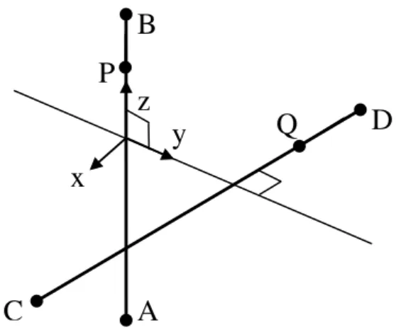
In the Pople-Hehre (PH) algorithm,² Cartesian axes are rotated to make z- and y- directions along AB and perpendicular to AB and CD, respectively, as shown in Fig. 1, which are named axes-2 in the original paper. Point P lies on the AB line and depends on exponents A and B. In the rotated coordinate, PAx, PAy, PBx, and PBy are zero and PQx and PQy become constant at any point P. QCy, and QDy are zero at any point Q.

Figure 1. Rotated Cartesian axes.

In the McMurchie-Davidson (MD) algorithm,⁶ the bra part of the primitive [ab|cd] (=[ab0|cd0]) is formed from the following recurrence relation,

 











 











z y B

C

D

A P

Q

where subscript i denotes a Cartesian direction (x, y, or z) and 1i is the unit vector of the i-direction. The ket part is also formed in the following way,









 







 



 

 _|

2

|

|

|  ¹ . (14)

[p|q] (=[00p|00q]) necessary to generate [ab|cd] is evaluated by

 

 





 



 





 



 

_{ }

 

Q P

m Q m m P

Q P d c b a m

2 1 1 1 2

5

2 1 _







 







 

0 (17)

where

 

_

0

2 ²

dt e t T

F_m ^{m Tt} (18)

 

Q P

Q

T P









  . (19) When T is small, Fm(T)for the largest m value is evaluated using Taylor or Chebyshev expansions and the others are evaluated using the following recurrence relation,¹⁸

  

 

 



T m

F_{m m}  

  2 _ exp

1 2

1

1 . (20) When T is large, F₀(T) is evaluated using the following equation,

 

F₀   4 , (21) and the others are evaluated using the following recurrence relation,

  

  

F_m1  2 1 _m 2 . (22) We developed the PH+MD algorithm by combining the PH and MD algorithms. Cartesian axes are rotated using the PH algorithm, as described above, and then ERIs are calculated using MD algorithm at the rotated coordinate. The calculated ERIs are

transformed to the original coordinate. The second rotation in the original PH algorithm, axes-1, is not exploited in the PH+MD algorithm because the rotation is not useful for contracted basis functions. The pseudocode is shown in Fig. 2. Cartesian axes are first rotated, as shown in Fig. 1, and the quadruple loop starts at the rotated coordinate. The outer loop is over c and d, and the inner loop is over a and b. In the quadruple loop, [0]^(m) and the related integrals such as (P_z-A_z)[0]^(m), (P_z-B_z)[0]^(m), (2P^{)-1[0](m), and}

(Q_z-P_z)[0]^(m) are calculated and accumulated. Calculations of integrals including terms such as (Px-Ax) and (Qy-Py) are skipped because PAx, PAy, PBx, and PBy are all zero and PQ_x and PQ_y are constant at the rotated coordinate. After the loop, the bra-contracted integrals (0]^(m) are obtained. In the double loop, (r] and the related integrals such as (Pz-Az)(r], (Qx-Cx)(r], and (2Q)^-1(r] are calculated and accumulated. Calculations of integrals including terms such as (Px-Ax) and (Qy-Cy) are again skipped because PAx, PA_y, PB_x, PB_y, QC_y, and QD_y are all zero. After the loop, the contracted integrals (r) are obtained. The (ab|cd) integrals are calculated from (r) using Eqs. 13-15 in the rotated coordinate and finally transformed into the original coordinate. (sp,sp|sp,sp) and (dd|dd) integrals have 90K⁴ and 830K⁴ constant values and 250K²+380 and 3900K²+31000 zero values, respectively (K is the degree of contraction).

As an example, we describe the (ps|ss) generation. In the quadruple loop, [0]⁽⁰⁾ and [0]⁽¹⁾ are calculated for each primitive function, and (2P^{)-1[0](1), (Q}z^-Pz)(2P^)-1[0](1),

and (P_z-A_z)[0]⁽⁰⁾ are calculated and accumulated for the bra part. In the double loop, (2P^)-1(x], (2P^)-1(y], (2P^)-1(z], and (P_z-A_z)(0] are calculated and accumulated for the ket part. After the loop, (ps|ss) integrals are calculated using the following recurrence relations derived from Eqs. 13-15,



 

  







  



 

  

  

rotate Cartesian axes do c shells

do d shells do a shells do b shells calculate Fm(T)

calculate and accumulate [0]^(m) and the related integrals enddo b

enddo a

calculate and accumulate (r]^(m) and the related integrals enddo d

enddo c

calculate (ab|cd)

rotate (ab|cd) to original Cartesian axes

Figure 2. Pseudocode of PH+MD algorithm.

1.4 Results

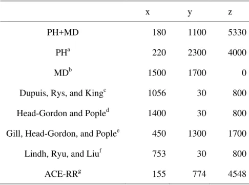
Tables 1 and 2 show the FLOP count parameters for (sp,sp|sp,sp) and (dd|dd), respectively. The FLOP count is given by

FLOPs = xK⁴ + yK² + z. (26)

Table 1. FLOP count parameters for (sp,sp |sp,sp).

^{x y z}

PH+MD 180 1100 5330

PH^a 220 2300 4000

MD^b 1500 1700 0

Dupuis, Rys, and King^c 1056 30 800

Head-Gordon and Pople^d 1400 30 800

Gill, Head-Gordon, and Pople^e 450 1300 1700

Lindh, Ryu, and Liu^f 753 30 800

ACE-RR^g 155 774 4548

aReference 2.

bReference 6.

cReference 3-5.

dReference 8.

eReference 9.

fReference 10.

gReference 17.

Table 2. FLOP count parameters for (dd |dd).

^{x y z}

PH+MD 850 11860 173500

MD^a 27300 24000 0

Dupuis, Rys, and King^b 30900 220 0

Head-Gordon and Pople^c 14600 30 11300 Gill, Head-Gordon, and Pople^d 2450 25800 28900

Lindh, Ryu, and Liu^e 10255 30 11300

ACE-b3k3^f 327 2281 163000

aReference 6.

bReference 3-5.

cReference 8.

dReference 9.

eReference 10.

fReference 12.

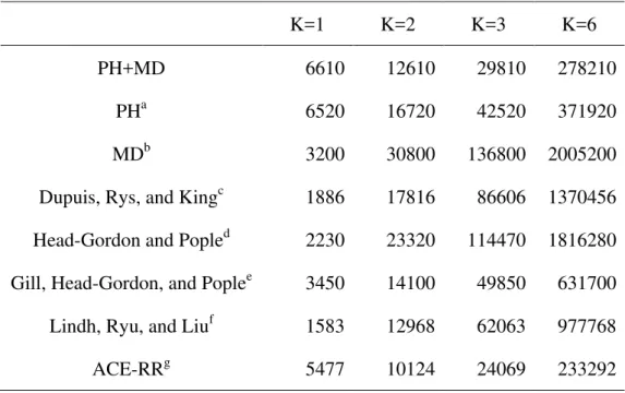
Table 3 shows the FLOP counts of (sp,sp|sp,sp) for several K. The parameters x and y for K⁴ and K² become very small in the PH+MD algorithm, compared with the original algorithms, because of zero components, constant components, and efficient recurrence relations. Instead, the zeroth power parameter z becomes large because the operations of the last recurrence relations, Eqs. 13-15, are performed. This PH+MD algorithm is especially suited for the moderate degree of contraction, for instance, STO-3G and 6-31G(d). The FLOP count of the PH+MD algorithm is not the least of all the algorithms. However more than 80% operations of the algorithm are performed in do

loops. This is a significant advantage for practical calculations because of the sequential access to fast memory.

Table 3. FLOP counts for (sp,sp |sp,sp).

^{K=1 K=2 K=3 K=6}

PH+MD 6610 12610 29810 278210

PH^a 6520 16720 42520 371920

MD^b 3200 30800 136800 2005200

Dupuis, Rys, and King^c 1886 17816 86606 1370456 Head-Gordon and Pople^d 2230 23320 114470 1816280 Gill, Head-Gordon, and Pople^e 3450 14100 49850 631700 Lindh, Ryu, and Liu^f 1583 12968 62063 977768

ACE-RR^g 5477 10124 24069 233292

aReference 2.

bReference 6.

cReference 3-5.

dReference 8.

eReference 9.

fReference 10.

gReference 17.

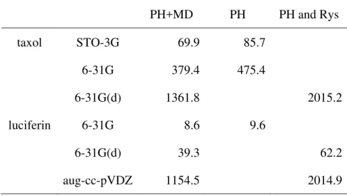
The PH+MD algorithm derived for (ss|ss) to (dd|dd) was implemented into the quantum chemistry package GAMESS¹⁹ by adding 39000 lines. Test calculations were performed for PH+MD and compared with the PH and Rys algorithms available in GAMESS using a 3.0GHz Pentium4 machine. PH is used for ERIs including s and sp functions and Rys is used for ERIs including d functions. The computational times for the Fock matrix generation in the first direct SCF iteration are shown in Table 4 for taxol (C₄₇H₅₁NO₁₄, no symmetry) and luciferin (C₁₁H₈N₂O₃S₂, no symmetry). STO-3G, 6-31G, and 6-31G(d) basis sets were used for taxol and 6-31G, 6-31G(d), and aug-cc-pVDZ were used for luciferin. An integral prescreening threshold of 10^-9 was adopted in all calculations. As shown in Table 4, the PH+MD algorithm reduces computational times by 10-20% in comparison with the PH algorithm for the STO-3G and 6-31G basis sets. This is because the FLOP count of (sp,sp|sp,sp) is 25-30% reduced in PH+MD though the FLOP counts of (ss|ss) and (sp,s|ss) are almost the same in PH+MD and PH. It is interesting that PH+MD reduces the computational times by 32-43% in comparison with PH and Rys for 6-31G(d) and aug-cc-pVDZ. This is owing to the fact that ERIs of sp and d functions such as (d,sp|d,sp) and (dd|sp,sp) are generated very fast. Only for primitive (dd|dd) calculations PH+MD is somewhat slower than Rys. The number of primitive (dd|dd) ERIs is usually very small, so that the disadvantage is negligible in practical calculations. Due to the small x coefficient for quartic work, the strength of this new approach must be even more apparent for heavy atoms with valence or core d electrons, whose basis sets would contain contracted d functions.

Table 4. Computational times of PH+MD, PH, and Rys algorithms (sec).

^{PH+MD PH} PH and Rys

taxol STO-3G 69.9 85.7

6-31G 379.4 475.4

6-31G(d) 1361.8 2015.2

luciferin 6-31G 8.6 9.6

6-31G(d) 39.3 62.2

aug-cc-pVDZ 1154.5 2014.9

1.5 Conclusions

A new algorithm to calculate (ss|ss) to (dd|dd) ERIs is developed by combining the PH and MD algorithms and implemented into the GAMESS program. The FLOP count is highly reduced because of the axis-switch in PH and the recurrence relation in MD. The PH+MD algorithm is considerably faster than the PH and Rys algorithms, especially for the basis sets including d functions such as 6-31G(d) and aug-cc-pVDZ.

1.6 References

1. Boys, S. F. Proc Roy Soc London A 1950, 200, 542. 2. Pople, J. A.; Hehre, W. J. J Comput Phys 1978, 27, 161. 3. King, H. F.; Dupuis, M. J Comput Phys 1976, 21, 144. 4. Dupuis, M.; Rys, J.; King, H. F. J Chem Phys 1976, 65, 111. 5. Rys, J.; Dupuis, M.; King, H. F. J Comput Chem 1983, 4, 154. 6. McMurchie, L. E.; Davidson, E. R. J Comput Phys 1978, 26, 218.

7. Obara, S.; Saika, A. J Chem Phys 1986, 84, 3963.

8. Head-Gordon, M.; Pople, J. A. J Chem Phys 1988, 89, 5777.

9. Gill, P. M. W.; Head-Gordon, M.; Pople, J. A. J Phys Chem 1990, 94, 5564. 10. Lindh, R.; Ryu, U.; Liu, B. J Chem Phys 1991, 95, 5889.

11. Ishida, K. Int J Quantum Chem 1996, 59, 209. 12. Ishida, K. J Comput Chem 1998, 19, 923.

13. Gill, P. M. W.; Pople, J. A. Int J Quantum Chem 1991, 40, 753. 14. Schlegel, H. B. J Chem Phys 1982, 77, 3676.

15. Hamilton, T. P.; Schaefer, III H. F. Chem Phys 1991, 150, 163. 16. Ten-no, S. Chem Phys Lett 1993, 211, 259.

17. Kobayashi, M.; Nakai, H. J Chem Phys 2004, 121, 4050.

18. Gill, P. M. W.; Johnson, B. G.; Pople, J. A. Int J Quantum Chem 1991, 40, 745. 19. Schmidt, M. W.; Baldridge, K. K.; Boatz, J. A.; Elbert, S. T.; Gordon, M. S.; Jensen, J. H.; Koseki, S.; Matsunaga, N.; Nguyen, K. A.; Su, S.; Windus, T. L.; Dupuis, M.; Montgomery, J. A. J Comput Chem 1993, 14, 1347.

Chapter II

A New Parallel Algorithm of MP2 Energy Calculations (Ishimura,K; Pulay, P.; Nagase S. J Comput Chem 2006, 27, 407.)

2.1 Abstract

A new parallel algorithm has been developed for second order Møller-Plesset perturbation theory (MP2) energy calculations. Its main projected applications are for large molecules, for instance for the calculation of dispersion interaction. Tests on a moderate number of processors (2-16) show that the program has high CPU and parallel efficiency. Timings are presented for two relatively large molecules, taxol (C₄₇H₅₁NO₁₄) and luciferin (C₁₁H₈N₂O₃S₂), the former with the 6-31G* and 6-311G** basis sets (1032 and 1484 basis functions, 164 correlated orbitals), and the latter with the aug-cc-pVDZ and aug-cc-pVTZ basis sets (530 and 1198 basis functions, 46 correlated orbitals). An MP2 energy calculation on C₁₃₀H₁₀ (1970 basis functions, 265 correlated orbitals) completed in less than 2 hours on 128 processors.

2.2 Introduction

Density functional theory (DFT) is currently the most widely used method to calculate molecular properties. However, the generally used local and semilocal DFT methods fail to describe the dispersion interaction that plays an important role for large molecules, and usually underestimate reaction barriers. The simplest method to include dispersion nonempirically is second order Møller-Plesset perturbation theory (MP2).¹ The formal scaling of MP2 with molecular size (assuming constant basis set quality) is fifth order, O(n⁵), higher than the O(n⁴) formal scaling of Hartree-Fock theory. Moreover, natural sparsity is more difficult to use in canonical MP2 theory than in Hartree-Fock theory. These factors together made MP2 theory significantly more costly for large systems than, say, Hartree-Fock theory. Much effort has been expended to create less expensive approximations to MP2. Local MP2^2-9 can be much less expensive than full MP2 for large systems. Other efficient methods include Density Fitting (Resolution of Identity, RI) MP2^10-13 and Laplace Transform MP2.^14-17 All of these methods include approximations that need to be carefully checked against full calculations. Most introduce a new model chemistry, and have limitations. For instance, the efficiency of local MP2 decreases for genuinely delocalized systems, like - interactions, and for diffuse basis sets. The recent implementation of RI-MP2 by the Ahlrichs group¹³ has no problems with large basis sets and promises to be an excellent tool for routine calculations. However, it also introduces a slightly different model chemistry, and its ultimate scaling is fifth order, like that of canonical MP2. A Laplace Transform MP2 utilizing natural sparsity has been implemented¹⁷ but its computational superiority has yet to be demonstrated.

An alternative method of overcoming the long computational times of MP2 is parallel implementation. This has become particularly useful with the advent of

inexpensive high-speed processors. A number of papers have been published on parallel integral transformation, the main part of parallel MP2.^18-28 The simplest parallelization methods use a single variable, say atomic orbital (AO) or molecular orbital (MO) indices to distribute the workload, or use shared memory computers. These methods have significant shortcomings. For instance, in the AO-based parallelization of Nielsen and Seidl²³ progressively more network communication is needed as the number of processors increases. The MO-based parallelization, for instance the methods devised by Schütz and Lindh²⁶ require the repeated evaluation of AO integrals on different nodes or to broadcast integrals to all nodes, limiting parallel efficiency. Shared memory computers are much less widely available and more expensive than clusters, and their size is limited.

Recently, Baker and Pulay²⁹ have described a parallel MP2 implementation, based on an efficient canonical program³⁰ using the Saebo-Almlöf integral transformation method.³¹ This program parallelizes the first half transformation by AO indices and the second half transformation by MO indices. Its advantages are that the fast memory needed scales only with the square of the system size, the total amount of communication is independent of the number of processors, and the AO integrals are generated only once. One of its disadvantages is that it uses only one permutational symmetry during AO integral generation, quadrupling the computational effort for this task. However, the main disadvantage of the Baker-Pulay code is the I/O overhead involved in the sorting of the half-transformed integrals. While disk I/O on the current generation of computers cannot be eliminated, the current project aims at reducing this overhead. The required memory in the present code has a cubic component. However, it is proportional to o²n only, where o is the number of correlated MOs. In most MP2 calculations, o is about an order of magnitude smaller than n, the number of basis

functions, and therefore memory becomes a limiting factor only for very large calculations in the present program.

The algorithm described in this paper has been implemented in the freely distributed quantum chemistry program system GAMESS.³² GAMESS has already a parallel MP2 implementation,²⁸ based on the Distributed Data Interface.³³ However, this implementation stores the transformed integrals, an array that scales with the fourth power of the molecular size, in distributed fast memory. If there is not enough memory, it resorts to expensive multiple passes. This is an efficient strategy on massively parallel computers where the aggregate memory is sufficient to hold all integrals, but it becomes inefficient for larger calculations on small or medium-sized clusters. By making use of ample and inexpensive disk storage, the program presented in this paper is able to perform large calculations on modest clusters with high efficiency.

2.3 Theory

The closed-shell MP2 energy can be written as

  _{   } ^{       }

   

 

 ^. 2 ^{. | 2 | |}

MP2 ^occ

j i

virt

ab i j a b

ij

ja ib jb ia jb E ia







  , (1)

where i and j are doubly occupied MOs, a and b are virtual MOs, and _{ε’s are} corresponding the orbital energies. (ia|jb) denotes a two-electron MO integral that is generated as

 

_  

 ^{   }



|

| jb C _iC_aC _jC _b

ia . (2)

Here, and in the following Greek letters denote AOs, (|) is a two-electron AO integral, and C is the matrix of the MO coefficients. The most time-consuming step in

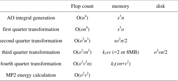
an MP2 energy calculation is the transformation of the AO integrals to MOs, Eq. (2). The outline of the new algorithm is summarized in Figure 1 and the required memory, disk space requirements, and formal computational costs are shown in Table 1. First, we describe the serial version. Capital Greek letters , , , and  denote shells of AOs; computational efficiency mandates the utilization of shell structure. The outermost loop up to the third quarter transformation is over AO shell . In the loop, AO integrals (|) are calculated for one , , and , and all . (|) denotes all integrals (|), , , , and . Schwartz prescreening^34-36 is used in this phase to discard insignificant integrals, just as in the SCF calculation. This results in significant computational savings. The required memory size in this step is s³n, where s is the maximum number of basis functions in a shell, for instance, 1 for s function and 4 for sp function and n is the total number of basis functions. The formal computational cost is O(n⁴); for large molecules, this diminishes to O(n²). Only one of the three permutational symmetries, (|)=(|), is exploited in our algorithm. This means that AO integrals are effectively evaluated four times. The SCF algorithm and some other MP2 algorithms can use three symmetries. However, we find, in agreement with Pulay et al.,³⁰ that sacrificing permutational symmetry of the AO integrals incurs only a modest penalty. After the calculation of AO integral blocks, the first quarter transformation,

 

_  

 ^







i| C_i | (3)

is performed for all i, and , , and . The memory size required to store the transformed integrals is s³o, where o is the number of correlated MOs, and the formal computational cost is O(on⁴). The second quarter transformation,

 

_  

 ^







i| j C _j i| (4)

is performed for all i and j(≤i), and for  and . The required memory size is so²n/2 and the formal computational cost is O(o²n³). This is the step with the largest memory demand in our algorithm. On a 32-bit computer, memory limits restrict the calculation to ~2000 basis functions and 200 occupied orbitals if the highest angular momentum functions are 6-component d functions. This limit can be exceeded (see below) at the cost of introducing multiple integral batches. The half-transformed (i|j) integrals are accumulated for all i, j(≤i), and , and for . The quarter-transformed (i|) integrals are screened prior to the transformation.

The third quarter transformation,

 

_  

 ^





i|bj C _b i| j (5)

is performed for all i, j(≤i), and b, and for . The three-quarter transformed integrals are collected in fixed-size bins that are written to disk when full. We use the compact DDI library³³ in GAMESS for communication, and achieve high CPU efficiency by choosing the bin size the same size of disk cache, for instance, 2 or 8 MB. This reduces disk I/O time significantly, as writing to the disk cache is more than ten times faster than to the disk itself. The computational cost of this step, both formal and actual, is O(o²vn²), where v is the number of virtual MOs. No screening of the (i|j) integrals is used in this transformation, as the canonical orbitals are usually delocalized, making the screening ineffective. The total disk storage required is o²vn/2, somewhat less that in Ref. 30 (o²n²/2). After the Μ loop has finished, all (i|bj) integrals have been calculated and stored.

In the fourth quarter transformation,

 

_  

 ^

i bj C

bj

ai| _a | , (6)

the outermost loop step is over batches of ij pairs. A block of (i|bj) integrals for all , b and a batch of ij pairs are read from disk and transformed. For a single (ij) orbital pair, this step requires a minimum array size of vn for storing the (i|bj) integrals and v² for (ai|bj), in addition to the storage of the SCF coefficient matrix. However, efficiency is higher if as many pairs are processed together as possible. The computational cost of this step is O(o²v²n). The computational cost of the MP2 energy calculation is O(o²v²). If the memory demand is too high, the program can use multiple passes in the calculation of AO integrals to the third quarter transformation, with the AO integrals recalculated in each pass. The maximum memory size depends on the shell size s.

This algorithm uses a two steps parallelization like in Ref. 29. In our algorithm, AO indices, (in reality shells,  in Figure 1), are distributed dynamically to each processor in the AO integral generation phase and subsequent phases up to the third quarter transformation. A subset of the three-quarter transformed (i|bj) integrals (all bs, all ij, ij and a subset of s) is stored on each node, with b running fastest, followed by ij and finally . The fourth quarter transformation and the MP2 energy calculation are parallelized by batches of occupied MO pairs ij. This parallelization is static, i.e. each process gets approximately the same number of ij pairs, because no cut-offs are included, and therefore the timings are the same for each pair. Prior to the fourth quarter transformation, each process reads its own three-quarter transformed integrals, and sends them, according to the ij indices, to the appropriate node. As a result, the  indices become scrambled; rather than reorder the integrals, each process reorders its copy of the AO coefficient matrix accordingly. In the final, computationally insignificant stage, the partial MP2 energies are accumulated on the master process. The required memory size for each quarter transformation is the same as the serial version and the disk storage size per process is o²vn/2n_proc, where n_proc is the number of the processors. The total

amount of network communication is o²vn, and it does not depend on the number of processors. This feature is suitable for the parallel computation. An in-core version is available for small molecules or a large number of processors, in which all (i|bj) integrals are stored in memory, not on disk.

Table 1. Flop count, required memory, and total disk space for each step.

Flop count memory disk

AO integral generation O(n⁴) s³n first quarter transformation O(on⁴) s³o second quarter transformation O(o²n³) so²n/2

third quarter transformation O(o²vn²) k₁sv (=2 or 8MB) o²vn/2 fourth quarter transformation O(o²v²n) k2(vn+v²)

MP2 energy calculation O(o²v²) k₁, k₂: batches of ij pair.

do  (distributed dynamically) do  = 1, nshells

do = 1, 

Schwartz prescreening of (|) integrals

calculate

_

_

_

_{ }

_

_

_





transform to

_

_{ }

_

_

_

end do  do all ij batch

transform to



 



_

_

end do ij batch end do 

do ij batch (distributed statically)

28

read





_

_

transform to



 







end do ij batch

accumulate MP2 energy

Figure 1. Outline of the parallel algorithm.

29

2.4 Results and Discussion

Test calculations on taxol (C47H51NO14, no symmetry) and luciferin (C11H8N2O3S2, no symmetry) were performed on a cluster of 3.0 GHz Pentium4 computers connected by gigabit Ethernet. Each node has 2GB dual-PC3200 DDR memory and a striped pair of 200GB disks, each with 8MB cache.

6-31G* and 6-311G** basis sets were used for taxol, and aug-cc-pVDZ and aug-cc-pVTZ basis sets were used for luciferin. Only the valence orbitals were correlated. Table 2 summarizes the details of the calculation (the number of basis functions, shells, correlated orbitals, virtual orbitals, and SCF cycles), and the required memory and disk size per process, and the total amount of network communication. Table 3 shows elapsed timings and speed-ups of SCF and MP2 single point calculations. An integral screening threshold of 10^-10 was used in all calculations on taxol and 10^-11 on luciferin. The tighter threshold is required in the latter calculation because of the near-singularity of the augmented basis sets for luciferin (the lowest eigenvalue of the overlap matrix is 6.6x10^-8).

As the data in Table 2 show, even the large calculation (taxol 6-311G**, almost 1500 basis functions) can be easily accommodated by a single PC. This calculation needs less than 1 GB of fast memory and about 200 GB of disk space.

Table 2. Details of the calculations.

taxol luciferin

6-31G* 6-311G** aug-cc-pVDZ aug-cc-pVTZ

Number of contracted basis functions 1032 1484 530 1198

Number of basis shells 350 514 206 328

Number of correlated orbitals 164 164 46 46

Number of virtual orbitals 806 1196 422 948

Number of SCF cycles 14 14 15 14

Required memory size per processor /GB 0.67 0.96 0.05 0.16

Total required disk size /GB 90 192 2 10

Total amount of network communication /GB 90 192 2 10

As the timings in Table 3 show, in spite of its steeper formal scaling, the computational time for MP2 energy is commensurate with the SCF time. The parallel scaling of the code is excellent up to the largest number of nodes we have tried: For instance, on 16 processors the elapsed time for the MP2 calculation is 15.4 times faster (in average) than the single-processor time. This is a consequence of the high CPU efficiency of the code (88-98% on 16 processors) which is defined as the ratio of master node CPU and elapsed times.

Table 3. Elapsed times^a and speed-ups of SCF and MP2 calculations (minutes).

Number of processors 1 2 4 8 16

Taxol 6-31G*

tscf^b 323.7(100%) 160.6(99%) 82.6(99%) 42.6(96%) 25.0(84%)

sscf^c 1.00 2.02 3.92 7.60 12.94

tmp2^d 611.3(90%) 305.0(90%) 152.1(91%) 78.5(88%) 38.7(89%)

smp2^e 1.00 2.00 4.02 7.78 15.80

6-311G**

tscf^b 1051.5(100%) 520.2(100%) 263.8(99%) 137.6(97%) 73.5(89%)

sscf^c 1.00 2.02 3.99 7.64 14.31

tmp2^d 1898.2(92%) 975.0(90%) 483.7(91%) 242.9(91%) 123.3(88%)

smp2^e 1.00 1.95 3.92 7.81 15.40

Luciferin aug-cc-pVDZ

tscf^b 305.3(100%) 159.5(100%) 77.8(100%) 39.1(99%) 20.0(97%)

sscf^c 1.00 1.91 3.92 7.81 15.26

tmp2^d 114.3(99%) 58.2(99%) 29.0(98%) 14.8(98%) 7.5(97%)

smp2^e 1.00 1.96 3.94 7.73 15.19

aug-cc-pVTZ

tscf^b 3814.1(100%) 2062.4(100%) 971.0(100%) 487.1(100%) 244.0(99%)

sscf^c 1.00 1.85 3.93 7.83 15.63

tmp2^d 1452.7(100%) 710.5(99%) 367.9(98%) 182.3(96%) 96.1(98%)

^{smp2e 1.00 2.04 3.95 7.97 15.12}

aCPU efficiency is shown in parentheses.

bElapsed time of SCF calculation.

cSpeed-up of SCF calculation.

dElapsed time of MP2 calculation.

eSpeed-up of MP2 calculation.

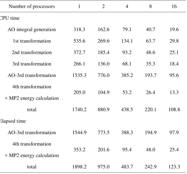
Table 4 shows the master node CPU and elapsed timings of the individual steps for the 6-311G** calculation on taxol. It is not possible to break down the elapsed time of the first steps (from AO integral generation to third transformation) and only the total is shown. Though the CPU timing ratios of the AO integral generation and each quarter transformation vary with the number of processors, the speed-up of the first step is almost proportional to the number of processors. The CPU efficiency of the first step is over 99%, in spite of writing the intermediate integrals on disk. This high efficiency is achieved by using an array size in the third transformation that is the same as the disk cache size. This way, the disk writing effectively overlaps with the CPU calculation. The lower CPU efficiency of the fourth transformation (including MP2 energy calculation) comes from reading the intermediate integrals from disk and from network communication. In this example, the CPU efficiency of the fourth transformation varies between 52% and 58%; it shows no systematic variation with the number of processors. The most time-consuming step is the first transformation for the 6-311G** basis, and the second transformation for the 6-31G* basis. As Table 4 shows, the ratio of the first to the second quarter transformation for the 6-311G** basis is only about 1.5, much less than the ratio n/o=9, showing the efficiency of integral screening. The percentages of the (|) integrals skipped in the first quarter transformation, and the (i|) integrals skipped in the second quarter transformation are 94.9% and 75.9% for 6-311G** and 93.4% and 72.6% for 6-31G* basis sets, respectively. The speed-ups on 2 processors, for instance, in luciferin aug-cc-pVTZ, are slightly higher than the

theoretical upper limit. It may happen that processor cache hit ratios on 2 processors are better than the ratios on 1 processor.

Table 4. CPU and elapsed times of each step for 6-311G** calculation on taxol (minutes).

Number of processors 1 2 4 8 16

CPU time

AO integral generation 318.3 162.6 79.1 40.7 19.6

1st transformation 535.6 269.6 134.1 63.7 29.8

2nd transformation 372.7 185.4 93.2 48.6 25.1

3rd transformation 266.1 136.0 68.1 35.3 18.4 AO-3rd transformation 1535.3 776.0 385.2 193.7 95.6

4th transformation

+ MP2 energy calculation ^{205.0 104.9 53.2 26.4 13.3}

total 1740.2 880.9 438.5 220.1 108.8

Elapsed time

AO-3rd transformation 1544.9 773.5 388.3 194.9 97.9 4th transformation

+ MP2 energy calculation ^{353.2 201.6 95.4 48.0 25.4}

total 1898.2 975.0 483.7 242.9 123.3

Figure 2 shows the speed-ups, defined as the ratios of elapsed times, of the 6-311G** calculation on taxol and the aug-cc-pVTZ calculation on luciferin. The speed-ups are