Search frictions and market power in negotiated price markets
∗Jason Allena Robert Clarkb Jean-Fran¸cois Houdec
Abstract
This paper provides a framework for the empirical analysis of negotiated-price markets in which buying is single-source. These markets pose a challenge for empirical work since, although buyers potentially negotiate with many sellers, data-sets typically include only accepted offers. Moreover, negotiated-price markets feature search frictions, since consumers incur a cost to gather quotes, and long-term relationships between consumers and incumbent sellers, leading to the development of brand loyalty. Together, these characteristics imply that many consumers fail to consider more than one option, and while firms with extensive consumer bases have an incumbency advantage. We use data from the Canadian mortgage market and a model of search and negotiation to characterize the impact of search frictions on consumer welfare and to quantify the role of search costs and brand loyalty for market power. Our results suggest that search frictions reduce consumer surplus by almost $12 per month per consumer, and that 28% of this reduction can be associated with discrimination, 22% with inefficient matching, and the remainder with the search cost. We also find that banks with large consumer bases have margins that are 70% higher than those with small consumer bases. The main source of this incumbency advantage is brand loyalty, however, the ability to price discriminate based on search frictions also accounts for almost a third of the advantage.
1
Introduction
In a large number of markets, sellers post prices, but actual transaction prices are achieved via bilateral bargaining. This is the case for instance in the markets for new/used cars (Goldberg (1996), Scott-Morton et al. (2001), and Busse et al. (2006)), health insurance (Dafny (2010)), capital assets (Gavazza (2016)), financial products (Hall and Woodward (2012) and Allen et al. (2014a)), as well as for most business-to-business transactions (e.g. Joskow (1987), Town and Vistnes (2001) and Salz (2015)).
In this paper, we are interested in two key features characterizing many of these markets. First, since buyers incur a cost to gather price quotes, these markets are characterized by important search frictions. Second, the repeated relationship that develops between a buyer and a seller creates aloyalty advantage, which increases the value of transacting with the same seller. This can be because of switching costs associated with changing suppliers, cost advantages of the incumbent sellers, or because of complementarities from the sale of related products.
Search frictions and brand loyalty have implications for market power. Search costs open the door to price discrimination: the seller offering the first quote is in a quasi-monopoly position, and can make relatively high offers to consumers with poor outside options and/or high expected search costs. Brand loyalty reduces the bargaining leverage of consumers, because incumbent sellers provide higher value, which creates a form of lock-in. Together, these features imply that a firm with an extensive consumer base has anincumbency advantageover rival firms in the same market. We study one particular negotiated-price setting, the Canadian mortgage market, for which we have access to an administrative data-set on a large number of individually negotiated mortgage contracts, which we use to estimate a model of search and price negotiation. In this market, national lenders post common interest rates, but in-branch loan officers have considerable freedom to negotiate directly with borrowers. Importantly, there is evidence of search frictions and brand loyalty in this setting. About 70% of consumers in this market combine day-to-day banking and mortgage services at their main financial institution and 80% get a rate quote from this lender. Moreover, despite the fact that approximately 60% of consumers search for additional quotes, only about 28% obtain a mortgage from a different lender than their main institutions.
In this setting, we consider two questions. First, what is the impact of search frictions on the welfare of consumers? Second, what are the sources and magnitude of market power? We focus on quantifying the incumbency advantage that stems from a large consumer base and decomposing it into two parts: (i) a first-mover advantage arising from price discrimination and search frictions, and (ii) a loyalty advantage originating from long-term relationships.
observe transaction prices, and the identity of sellers, including whether or not buyers remain loyal to their current supplier. This poses a serious challenge for empirical work, since the outside option of buyers is unobserved.1 In our case-study, we do not observe rejected offers, or whether consumers
search for more than one lender. This is not unique to mortgage lending; most data-sets used in previous empirical work on price negotiation in consumer goods and business-to-business markets share these same features.2
To overcome these challenges, we use a two-stage search model in which individuals are initially matched with their home bank for a quote, and then decide, based on their expected net gain from searching, whether or not to gather additional quotes. The home bank uses this initial quote to price discriminate by screening high search-cost consumers. If it is rejected, consumers pay a search cost, and local lenders compete via an English auction for the contract. Using an auction to characterize the competition stage represents a tractable approach to address the missing prices problem. In particular, it accounts for the fact that sellers, in most price negotiation markets, are able to counter rivals’ offers by lowering prices; a process which mimics an English auction. This modeling strategy is related to search and bargaining models with asymmetric information developed by Wolinsky (1987), Chatterjee and Lee (1998), and Bester (1993), in which consumers negotiate with one firm, but can search across stores for better prices.
The tractability of the model also allows us to analyze the identification of the parameters in a transparent way. In particular, we discuss the conditions under which the distributions of search-and lending-costs are non-parametrically identified, using insights from the labor, discrete-choice and empirical auctions literatures. The identification argument is generalizable to other negotiated-price settings in which researchers have access to data on transaction negotiated-prices and switching decisions (but not necessarily search). Although the search- and lending-cost distributions could in theory be non-parametrically estimated, we instead estimate a parametric version of the model using maximum likelihood. This allows us to more easily incorporate observable differences between consumers and firms.
The results can be summarized as follows. We find that firms face relatively homogeneous lending costs for the same borrower. In contrast, we find that borrowers face significant search costs and brand loyalty advantage. On average, consumers in our sample face an upfront search cost of $1,150. In addition, the incumbent bank has an average cost advantage of $17.10/month (for a $100K loan) generating a sizeable loyalty advantage.
1As a result we cannot use recent approaches based on the simultaneous complete-information multi-lateral nego-tiation game proposed by Horn and Wolinsky (1988) that have modeled the outside option as observed prices paid by a given buyer to alternative suppliers (Crawford and Yurukoglu (2012), Grennan (2013), Lewis and Pflum (2015), Gowrisankaran et al. (2015) and Ho and Lee (2017)).
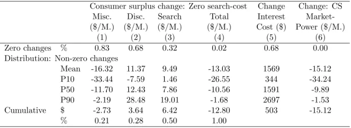
We use the model estimates to characterize the impact of search frictions on consumer welfare and to measure market power. To quantify the welfare cost of search frictions, we perform a set of counter-factual experiments in which we eliminate the search costs of consumers. The surplus loss from search frictions originates from three sources: (i) misallocation of buyers and sellers, (ii) price discrimination, and (iii) the direct cost of gathering multiple quotes. Our results suggest that search frictions reduce average consumer surplus by almost $12 per month, over a five year period. Approximately 28% of the loss in consumer surplus comes from the ability of incumbent banks to price discriminate with their initial quote. A further 22% is associated with the misallocation of contracts, and 50% with the direct cost of searching. We also find that the presence of a posted-rate limits the ability of firms to price discriminate, thereby reducing the welfare cost of search frictions. Competition also amplifies the adverse effects of search frictions on consumer welfare.
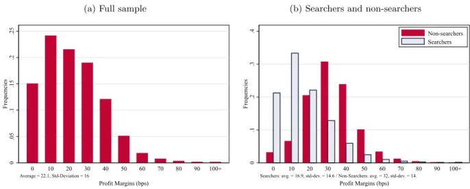
Our results also suggest that the market is fairly competitive. The average profit margin is estimated to be just over 20 basis points (bps), which corresponds to a Lerner index of 3.2%. However, margins vary considerably depending on whether consumers search and/or switch. On average, firms charge a markup that is 90% higher for consumers who are not searching. Banks’ profits from switching consumers are $14.99/month (17.1 bps), compared to $20.22/month from loyal consumers (24.6 bps).
The increased profits earned from loyal consumers correspond to the incumbency advantage, and are directly related to the size of the bank’s consumer base. To measure the source and magnitude of the advantage we use the simulated model to evaluate the correlation between consumer base and its profitability. We find that banks with the largest consumer bases earn, on average, 62% of the profits generated in their markets, compared to only 2% for those with the smallest. This difference is driven by the fact that large consumer-base lenders control a large share of the mortgage market, and earn significantly more profit per contracts than smaller banks.
We measure the incumbency advantage as the increased market power of banks with large consumer bases relative to those with the smallest. Our estimates suggest that banks with large consumer bases have margins that are 70% higher than those with small consumer bases. To identify the importance of the two sources of the incumbency advantage we simulate a series of counter-factual experiments aimed at varying the first-mover advantage and the differentiation component independently. Our results suggest that about 50% of the incumbency advantage can be directly attributed to brand loyalty, 30% to search frictions and the remaining 20% to their interaction.
and Syverson (2004), Hong and Shum (2006), Wildenbeest (2011), De Los Santos et al. (2012), Honka (2014), Alexandrov and Koulayev (2017), and Marshall (2016)). Although these papers take into account concentration and differentiation, they have mostly focused on cases where firms offer random posted prices to consumers irrespective of their characteristics (as opposed to targeted negotiated price offers). Lastly, our findings contribute to the literature on the advantages accruing to incumbent firms from demand inertia and brand loyalty. Bronnenberg and Dub´e (2016) provide an extensive survey of this literature in I.O. and marketing. Our model allows us to quantify the relative importance of two sources of state dependence, and the market-power associated with the incumbency advantage.
The paper is organized as follows. Section 2 presents details on the Canadian mortgage market and introduces our data sets. Section 3 presents the model, and Section 4 discusses conditions for non-parametric identification of the primitives. Section 5 discusses the estimation strategy and Section 6 describes the empirical results. Section 7 analyzes the impact of search friction and brand loyalty on consumer welfare and market power. Finally, section 8 concludes.
2
Institutional details and data
2.1 Institutional details
The Canadian mortgage market is dominated by six national banks (Bank of Montreal, Bank of Nova Scotia, Banque Nationale, Canadian Imperial Bank of Commerce, Royal Bank Financial Group, and TD Bank Financial Group), a regional cooperative network (Desjardins in Qu´ebec), and a provincially owned deposit-taking institution (Alberta’s ATB Financial). Collectively, they control 90% of banking industry assets. For convenience we label these institutions the “Big 8.”
Canada features two types of mortgage contracts – conventional, which are uninsured since they have a low loan-to-value ratio, and high loan-to-value, which require insurance (for the lifetime of the mortgage). Most new home-buyers require mortgage insurance. The primary insurer is the Canada Mortgage and Housing Corporation (CMHC), a crown corporation with an explicit guarantee from the federal government. During our sample period a private firm, Genworth Financial, also provided mortgage insurance, and had a 90% government guarantee. CMHC’s market share during our sample period averages around 80%. Both insurers use the same insurance guidelines, and charge lenders an insurance premium, ranging from 1.75% to 3.75% of the value of the loan, which is passed on to borrowers.3
The large Canadian banks operate nationally and their head offices post prices that are common across the country on a weekly basis in both national and local newspapers, as well as online. Throughout our entire sample period the posted rate is nearly always common across lenders, and
represents a ceiling in the negotiation with borrowers.4
According to data collected by marketing firm Ipsos-Reid, the majority of Canadians have a main financial institution where they combine checking and mortgage accounts. Therefore, potential borrowers can accept to pay the rate posted by their home bank, or search for and negotiate over rates. Borrowers bargain directly with local branch managers or hire a broker to search on their behalf.5 Our model excludes broker transactions and focuses only on branch-level transactions.
2.2 Mortgage data
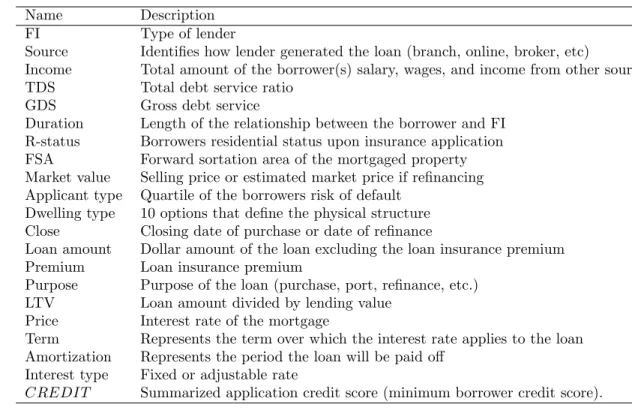
Our main data set is a 10% random sample of insured contracts from the CMHC, from January 1999 to October 2002. The data-set contains information the terms of the contract (transaction rate, loan size, and house price), as well as financial and demographic characteristics of the borrower. In the empirical analysis we focus in particular on the income of the borrower, the FICO risk score, the loan-to-value ratio, and the 5-year bond-rate valid at the time of negotiation. In addition, we observe the closing date of the contract and the location of the purchased house up to the forward sortation area (FSA).6,7
The data set contains the lender information for twelve of the largest lenders during our sample period. For mortgage contracts where we do not have a lender name but only a lender type, these are coded as “Other credit union”, and “Other trusts”. The credit-union and trust categories are fragmented, and contain mostly regional financial institutions.8 We therefore combine both into a
single “Other Lender” category. Overall, therefore, consumers face 12 lending options.
We restrict our sample to contracts with homogenous terms. In particular, from the original sample we select contracts that have the following characteristics: (i) 25-year amortization period, (ii) 5-year fixed-rate term, (iii) newly issued mortgages (i.e. excluding refinancing), (iii) contracts that were negotiated individually (i.e. without a broker), (iv) contracts without missing values for key attributes (e.g. credit score, broker, and residential status).
The final sample includes around 26,000 observations, or about one-third of the initial sample. Approximately 18% of the initial sample contained missing characteristics; either risk type or busi-ness originator (i.e. branch or broker). This is because CMHC started collecting these transaction
4In Canada pricing over the posted rate is illegal, and therefore this is a natural assumption. A similar setup is implied in other retail markets featuring negotiation in the presence ofmanufacturer’s suggested retail prices.
5Local branch managers compete against rival banks, but not against other branches of the same bank. Brokers are “hired” by borrowers to gather the best quotes from multiple lenders but compensated by lenders.
6The FSA is the first half of a postal code. We observe nearly 1,300 FSA in the sample. While the average FSA has a radius of 7.6 kilometers, the median is 2.6 kilometers.
7Based on the closing date we construct a posted price associated with each contract as the posted rate at closing if this yields a non-negative discount. If the generated discount is negative, the posted rate is taken to be the nearest-one that yields a positive discount.
characteristics systematically only in the second half of 1999. We also drop broker transactions, (28%), as well as short-term, variable rate and refinanced contracts (40%).
We use the data to construct three main outcome variables: (i) monthly payment, (ii) nego-tiated discounts, and (iii) loyalty. The monthly payment, denoted by pi, is constructed using the transaction interest rate, loan size, and the amortization period (60 months) specified in borrower
i’s contract. To construct negotiated discounts, we must first identify the posted rate valid at the time of negotiation. Since our contract data include only the closing date, to pin down the appropriate posted rate we infer the negotiation week that maximizes the aggregate fraction of con-sumers paying the posted rate (or 33 days prior to closing). Lastly, the loyalty variable is a dummy variable equal to one if a consumer has prior experience dealing with the chosen lender. Since 75% consumers are new home buyers, this most likely identifies the bank with which the borrower possess a savings or checking account. Note that this variable is not available for one lender, and we therefore treat the loyalty outcome as partly missing when constructing the likelihood function Finally, since the main dataset does not provide direct information on the number of quotes gathered by borrowers, we supplement it with survey evidence from the Altus Group (FIRM survey). The survey asks 841 people who purchased a house during our sample period about their shopping habits. We use the aggregate results of this survey to construct auxiliary moments characterizing the fraction of consumers who report searching for more than one lender, by demographic groups. We focus in particular on city size, regions, and income groups.
2.3 Market-structure data
The market structure is described by the consumer base of each bank, and the number of lenders available in consumers’ choice sets. The consumer base of a lender is defined by its share of the market for day-to-day banking services. In the model, this is used to approximate the fraction of consumers in a given market that have prior experience with each potential lender. To construct this variable, we use micro-data from a representative survey conducted by Ipsos-Reid.9 Each year, Ipsos-Reid surveys nearly 12,000 households in all regions of the country. We group the data into by year, regions (10), and income categories (4). Within these sub-samples we estimate the probability of a consumer choosing one of the twelve largest lenders as their main financial institution, or home bank denoted byh. We use ψh(xi) to denote the probability that a consumer with characteristics
xi has prior experience with bankh.
The choice set of consumers is defined by the location of the house being purchased. In partic-ular, we assume that consumers have access to lenders that have a branch located within 10 KM of the centroid of their FSAs.10 This choice is justified by the data: over 90% of loans are originated
9Source: Consumer finance monitor (CFM), Ipsos-Reid, 1999-2002.
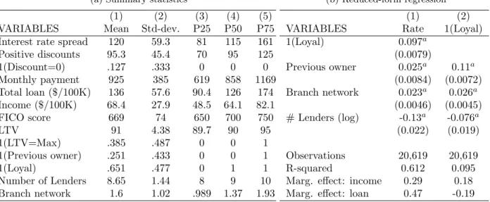
Table 1: Descriptive statistics on mortgage contracts and loyalty in the selected sample
(a) Summary statistics
(1) (2) (3) (4) (5)
VARIABLES Mean Std-dev. P25 P50 P75
Interest rate spread 120 59.3 81 115 161
Positive discounts 95.3 45.4 70 95 125
1(Discount=0) .127 .333 0 0 0
Monthly payment 925 385 619 858 1169
Total loan ($/100K) 136 57.6 90.4 126 174
Income ($/100K) 68.4 27.9 48.5 64.1 82.1
FICO score 669 74 650 700 750
LTV 91 4.38 89.7 90 95
1(LTV=Max) .385 .487 0 0 1
1(Previous owner) .251 .433 0 0 1
1(Loyal) .651 .477 0 1 1
Number of Lenders 8.65 1.44 8 9 10
Branch network 1.6 1.02 .989 1.37 1.93
(b) Reduced-form regression
(1) (2)
VARIABLES Rate 1(Loyal)
1(Loyal) 0.097a
(0.0079)
Previous owner 0.025a
0.11a (0.0084) (0.0072)
Branch network 0.023a
0.026a (0.0046) (0.0045) # Lenders (log) -0.13a
-0.076a (0.022) (0.019)
Observations 20,619 20,619
R-squared 0.612 0.095
Marg. effect: income 0.29 0.18
Marg. effect: loan 0.47 -0.19
Sample size = 26,218. Number of missing loyal observations = 5,599. The sample covers the period from Jan 1999 to Oct 2002. We trim the top and bottom 0.5% of observations in terms of income and loan size. Interest rates and discounts are expressed in percentage basis points (bps). The number of lenders is within 10KM of the borrowers new home (neighborhood). Relative branch is defined as the average network size of the chosen institution relative to the average size of others present in the same neighborhood. Each regression also includes market and quarter/year fixed-effects, and other financial characteristics (i.e. posted-rate, bond-rate, FICO score, LTV, 1(LTV Max), loan size, income, loan/income.). Robust standard errors in parenthesis. Significance levels: ap<0.01,bp<0.05,cp<0.1.
by a lender present within 10 KM of each FSA. In addition, the fact that rates are negotiated directly with loan officers limits the ability of consumers to perform the transaction online. Indeed, CMHC reports that less than 2% of mortgages are originated through the internet or phone.
The location of each financial institution’s branches is available annually from Micromedia-ProQuest. We use this data set to match the new house location with branch locations, and construct each consumer’s choice set. Formally, a lender is part of consumer i’s choice set if it has a branch located within less than 10 KM of the house location. We useNi to denote the set ofrival lenders available to consumeri(excluding the home bank), while ni is the number of banks inNi.
2.4 Market features
Before introducing the model, we provides descriptive evidence outlining the key features of the Canadian mortgage market that we want to capture. Table 1a describes the main financial and demographic characteristics of the borrowers in our sample. Table 1b reports a subset of the coefficients of two reduced-form regressions describing the relationship between transaction char-acteristics and negotiation rates, as well as the probability of remaining loyal to the home bank.
The loan-to-value (LTV) variable shows that many consumers are constrained by the minimum down-payment of 5% imposed by the government guidelines. Nearly 40% of households invest the minimum. Our focus is on the monthly payment made by a borrower, and so when we talk about quotes and rates, they will be based on a given monthly payment. The average monthly payment made by borrowers in our sample is $925.
In what follows we present five key featuresthat characterize shopping behavior and outcomes in the Canadian mortgage market and most negotiated-price markets:
Feature 1: Mortgage transaction rates are dispersed. There is little within-week dispersion in posted prices, especially among the big banks, where the coefficient of variation on posted rates is very close to zero. In contrast, the coefficient of variation on transaction rates is 50%, and there is substantial residual dispersion as illustrated by the R2 of 0.61 in Table 1b. See Allen et al.
(2014b) for more details.
Feature 2: Consumers who are loyal and located in concentrated markets tend to pay higher rates. The rate regression shows that clients who remain loyal to their home bank receive discounts that are about 9.1 bps smaller than do new clients. It also shows that discounts are increasing in the number of local lenders and decreasing in relative network size.
Feature 3: Consumers search more than they switch. The search and negotiation process typically begins with the consumer’s main financial institution—about 80% of consumers get a quote from their main institution (see Allen et al. (2014a)). A little over 60% of consumers search, but only about 28% switch away from their main institution.
Feature 4: Consumers are more loyal in concentrated markets and to banks with larger branch networks. The loyalty regression shows that the likelihood of remaining loyal is decreasing in the number of lenders present in the market and increasing in relative network size.
Feature 5: Lenders with strong retail presence have larger market shares. On average consumers face 8.6 lenders within their neighborhood. Consumers tend to choose lenders with large branch networks; transacting with lenders that are nearly 60% larger than their competitors in terms of branches. Lenders with larger branch networks also tend to have a bigger share of the day-to-day banking market, generating a link between day-to-day market share and mortgage-market share that provides large banks with an incumbency advantage.
3
Model
reject this quote based on their heterogeneous search costs and their expected gain from gathering multiple quotes, which depends, among other things, on how competitive is their local market.
In addition to capturing these features, the model takes into account the fact that, during negotiation, loan officers can lower previously made offers in an effort to attract or retain potential clients. Furthermore, competition takes place locally between managers of competing banks, since consumers must contact loan officers directly to obtain discounts. We also suppose that branches that are part of the same network do not compete for the same borrowers, a feature of the Canadian mortgage market and of some, but not all, negotiated-price markets.
The next three subsections describe the model. First, we present preferences and cost functions, and the bargaining protocol. Then, we solve the model backwards, starting with the second stage of the game in which banks compete for consumers. Finally, we describe the consumer search decision, and the process generating the initial quote. All variables introduced in the model vary at the consumer level, i, based on observed or unobserved characteristics. To simplify notation we omit the borrower’s index i, and will add it back in the next section for random variables and consumer characteristics.
3.1 Preferences and cost functions
Consumers solve a discrete-choice problem over which lender to use to finance their mortgage:
max
j∈J vj−pj, (1)
whereJ is the set of lenders offering a quote,pj denotes the monthly payment offered by lenderj, and vj denotes the maximum willingness-to-pay (or WTP) associated with bankj.
The choice set J is defined both by where consumers live, and by their search decision. In particular, consumers can obtain a quote from their home bank (h) and from the nlenders in N. We assume that the cost of obtaining a quote from the home bank is zero, while the cost of getting additional quotes is κ > 0. This search cost does not depend on the number of quotes, and is distributed in the population according to CDFH(·).
The WTP of consumers is a combination of differentiation and mortgage valuation:
vj =
v+λ ifj=h, v else.
The valuation for a mortgage, v, is common across all lenders. Throughout we assume that it is large enough not to affect the set of consumers present in our sample. The parameter λ ≥ 0 measures consumers’willingness to pay for their home bankrelative to other lenders.
future benefits associated with selling complementary services to the borrower.11 Since we do not
observe the performance of the contract along the risk and complementarity dimensions, we use a reduced-form function to approximate the net present value of the contract. In particular, the monthly cost for bank j to lend to the consumer is:
cj =
c−∆ If j=h,
c+ωj If j6=h,
(2)
wherec is the common cost of lending to the consumer;ωj the cost differential of lenderj relative to the home bank (or its match value); and ∆ is the home bank’s cost advantage. This advantage arises because of the multi-product nature of financial institutions and the fact that the home bank is potentially already selling profitable products to the consumer.12 It could come from real complementarities generated by bundling products (economies of scope), and/or from the fact that costs include not just the direct cost of mortgage lending, but also revenues/costs derived from the sale of additional products.13 In contrast to the home bank, competing lenders may need to offer discounts on these products to overcome the switching costs on these products, or may not earn any revenues at all from them if consumers do not switch.
As we will see below, the importance of brand loyalty in the market is driven by the sum of the cost and willingness-to-pay advantage of the home bank: γ = ∆ +λ. We refer to γ as the home-bankloyalty advantage.
The idiosyncratic component, ωj, is distributed according to G(·), with E(ωj) = 0. We use subscript (k) to denote thekth lowest cost match value amongst the non home-bank lenders. The CDF of thekth order statistic among the nlenders is given by G
(k)(w|n) = Pr(ω(k) < w|n).
Finally, lenders’ quotes are constrained by a common posted price p.14 The posted price
deter-mines both the reservation price of consumers (i.e. v > p), and whether or not consumers qualify for a loan at a given lender (i.e. p > cj).
11While lenders are fully insured against default risk, the event of default implies additional transaction costs to lenders that lower the value of lending to risky borrowers. Pre-payment risk is perhaps more relevant in our context, since consumers are allowed to reimburse up to 20% of their mortgage every year without penalty.
12For instance, credit cards have a 50%-60% return on equity (ROE), compared to Canadian banks’ overall ROE of 16%.
13Note that we rule out the possibility that the incumbent bank has more information than other lenders, since otherwise, the problem would involve adverse selection, and the initial quote would be much more complicated. For a discussion about competition when one firm has more information about a consumer learned from their past purchases see Fudenberg and Villas-Boas (2007). A subset of this literature has focused on credit markets and the extent to which lenders can learn about the ability of their borrowers to repay loans and use this information in their future credit-decisions and pricing. See for instance Dell’Ariccia et al. (1999).
3.2 Bargaining protocol, information and timing of the game
In an initial period outside the model, consumers choose the type of house they want to buy, the loan size, L, and the timing of the home purchase (including closing date). Our focus is on the negotiation process, which we model as a two-stage game. In the first-stage, the home bank makes an initial offer p0. At this point, the borrower can accept the offer, or search for additional quotes
by paying the search cost κ. If the initial quote is rejected, the borrower organizes an English auction among the home bank and the n other banks present in their neighborhood. The lender choice maximizes the utility of consumers, as in equation (1).
Information about costs and preferences is revealed sequentially. At the initial stage, all parties observe the posted price p, the number of rival banks n, the common component of the lending cost c, and the home-bank cost and WTP advantages (λ,∆). These variables define the observed state vector: s = (c, λ,∆, p, n). This information is common to all players. The search cost is privately observed by consumers. The home bank knows only the distribution, which can vary across consumers based on observed demographic attributes. Finally, in the second stage of the game, each lender learns its idiosyncratic lending cost,ωj.
Before solving the game, two remarks are in order. First, consumers are price takers in the model, and so lenders have full bargaining power. This does not mean, however, that consumers have no bargaining leverage, since they have an informational advantage from knowing their search cost. This prevents the home bank from extracting the entire surplus of consumers, as in Allen et al. (2014a).15 Second, consumers are assumed to pay the cost of generating offers at the auction
stage (rather than firms). Therefore banks that are not competitive relative to the home bank are, in theory, indifferent between submitting and not submitting a quote. In these cases we assume that banks always submit a truthful offer that is consistent with their realized match values.
Next, we describe the solution of the negotiation by backward induction, starting with the competition stage.
3.3 Competition stage
Conditional on rejectingp0, the home bank competes with lenders in the borrower’s choice set. We model competition as an English auction with heterogeneous firms, and a cost advantage for the home bank.16 Since the initial quote can be recalled, firms face a reservation price: p0≤p.
We can distinguish between two cases leading to a transaction: (i) ¯p < c−∆, and (ii) c <
15Beckert et al. (2016) take a different approach, by assuming that consumers and firms split theknownsurplus from the auction using a Nash-Bargaining protocol. In this context, the relative bargaining power of consumers, instead of the search cost distribution, determines the split of the surplus.
p0 + ∆≤ p+ ∆. In the first case the borrower does not qualify at the home bank. A borrower
not qualifying at their home bank, must search and their reservation price is ¯p. This borrower may qualify at other banks because of differences inωj. The lowest qualifying cost bank wins by offering a price equal to the lending cost of the second most efficient qualifying lender:
p∗= min{c+ω(2),p¯}. (3)
This occurs if and only if, 0<p¯−c−ω(1).
If the borrower qualifies at the home bank, the highest surplus bank wins, and offer a quote that provides the same utility as the second best option. The equilibrium pricing function is:
p∗ =
p0 If ¯v+λ−p0 ≥v¯−c−ω(1)
c+ω(1)+λ If ¯v+λ−p0 <v¯−c−ω(1)<¯v−c+γ
c−γ ¯v−c−ω(1) >v¯−c+γ >v¯−c−ω(2) c+ω(2) If ¯v−c−ω(2)>v¯−c+γ.
(4)
This equation highlights the fact that, at the competition stage, lenders directly competing with the home bank will on average have to offer a discount equal to the loyalty advantage in order to attract new customers.17 In cases 1 and 2 the home bank provides the highest utility and so wins the auction. In case 1, the initial quote provides higher utility than does the next best lender’s quote and so the consumer paysp0. In case 2, the reverse is true and so the consumer pays
c+ω(1) +λ and gets utility of ¯v−c−ω(1). In cases 3 and 4, the home bank is not the highest
surplus lender and the consumer paysc−γ orc+ω(2) depending on whether the home bank is the second or third highest surplus lender.
3.4 Search decision and initial quote
The borrower chooses to search by weighing the value of accepting p0, or paying a sunk cost κ in
order to lower their monthly payment. The utility gain from search is:
¯
κ(p0, s) = ¯v+λ1−G(1)(−γ)
−Ep∗|p0, s
| {z }
2ndstage expected utility
−v¯+λ−p0
| {z }
1ststage utility = p0−Ep∗|p0, s−λG(1)(−γ),
where 1−G(1)(−γ) is the retention probability of the home bank in the competition stage. A consumer will rejectp0 if and only if the gain from search is larger than the search cost. Therefore, the search probability is:
Pr κ < p0−Ep∗|p0, s−λG(1)(−γ|n) ≡H κ¯(p0, s). (5)
Lenders do not commit to a fixed interest rate, and are open to haggling with consumers based on their outside options. This allows the home bank to discriminate by offering the same consumer up to two quotes: (i) an initial quotep0, and (ii) a competitive quote p∗ if the first is rejected.
The price discrimination problem is based on the expected value of shopping and the distribution of search costs. More specifically, anticipating the second-stage outcome, the home bank chooses
p0 to maximize its expected profit:
max p0≤p¯ (p
0−c+ ∆)[1−H(¯κ(p0, s))] +H(¯κ(p0, s))E(π∗
h|p0, s),
whereE(π∗
h|p0, s) = (p0−c+ ∆)(1−G(1)(p0−λ−c)) +
Rp0−c−λ
−γ (ω(1)+γ)dG(1), are the expected profits from the auction for the home bank. The first term represents the case where the initial quote provides higher utility than the next highest surplus lender, while the second is the reverse. Importantly, the home bank will offer a quote only if it makes positive profit at the posted-price: 0< p−c+∆. In the interior solution, the optimal initial quote is implicitly defined by the following first-order condition:
p0−c+ ∆ = 1−H(¯κ(p
0, s))
H′(¯κ(p0, s))¯κ
p0(p0, s)
| {z }
Search cost distribution
+ E(πh∗|p0, s)
| {z }
Cost and quality Differentiation
+ H(¯κ(p
0, s))
H′(¯κ(p0, s))¯κ
p0(p0, s)
∂E(πh∗|p0, s)
∂p0
| {z }
Reserve price effect
, (6)
where ¯κp0(p0, s) = ∂¯κ(p 0,s)
∂p0 . Equation (6) implicitly defines the home bank’s profit margins from price discrimination. It highlights three sources of profits: (i) positive average search costs, (ii) market power from differentiation in cost and quality (i.e. match value differences and home-bank cost advantage), and (iii) the reserve price effect. If firms are homogenous, the only source of profits will stem from the ability of the home bank to offer higher quotes to high search cost consumers.
Although the initial quote does not have a closed-form solution, in the following proposition (proven in Appendix B) we claim that, in the interior, it is additive in the common cost shock. This simplifies the problem, since we need to numerically solve the first-order condition for only one value of cper consumer.
From this proposition, we can characterize the initial quote as follows:
p0(s) =
¯
p Ifc >p¯−µ(∆, λ, n),
c+µ(∆, λ, n) Else.
To summarize, the model predicts three equilibrium functions: (i) the initial quote p0(s), (ii) the search-cost threshold ¯κ(s), and (iii) the competitive price p∗(ω, s). Although it is difficult to characterize these functions analytically, the separability of the initial quote in the interior leads to a series of useful predictions that are summarized in Corollary 1. We use these implications in the identification section below.
Corollary 1. The following predictions about the distribution of prices and search probability in the interior, when p0(s)<p¯, follow from Proposition 1:
(i) The equilibrium search probability is independent of c.
(ii) The equilibrium search probability is affected symmetrically by λand ∆. (iii) The distribution of p∗ for switchers is only a function of γ =λ+ ∆.
(iv) The average transaction price paid by loyal consumers is affected asymmetrically by λ and∆, and the effect of λ is stronger.
4
Identification
The model contains four primitives: (i) the distribution of the common lending cost conditional on observed attributes of borrower i and region and period fixed effects (xi), F(ci|xi), (ii) the distribution of idiosyncratic cost differences, G(ωij), (iii) the search-cost distribution, H(κi), and (iv) the loyalty-advantage parameters, (λ,∆). From the model description, we maintain the as-sumptions that the lending cost function is additively separable in c and ω, and that κi and ωij are IID. We also assume that loyalty parameters are common across consumers, and that (κi, ωij) are independent of observed borrower characteristics xi (this last assumption is partially relaxed in the empirical analysis).
In this section we discuss nonparametric identification of the search and cost distributions, as well as the identification of the loyalty parameters. In the next, we estimate a parametric version of the model, which allows us to more easily incorporate observable differences between consumers and firms.
The data correspond to a cross section of transaction prices, borrower characteristics, and lender choices (including whether or not the lender is the home bank). The characteristics of the borrower allow us to infer the posted price valid at the time of the transaction (¯pt(i)), as well
distribution of transaction prices given (xi,p¯t(i), ni) separately for switching and loyal consumers.
These three distributions correspond to the reduced form of the model.
We face two challenges when when discussing the mapping from the reduced form to the primi-tives of the model. First, since we only observe accepted offers, and we must infer the distributions of the two unobserved heterogeneity components (ci and ωi) from a single price. Second, since we do not observe search and switch decisions separately, we need to distinguish between two sources of attachment to the home bank–search costs and the loyalty advantage–solely using the conditional probability of remaining loyal to the home bank.
To overcome these challenges, in addition to the assumptions listed above, we rely on two exclusion restrictions. We assume that the number of lenders and the posted price are independent of the ci, conditional on the observed attributes of the borrower,xi. Furthermore, we require that both variables exhibit enough variation across borrowers. We formally introduce these assumptions in Appendix C, and propose a sequential approach to show that they are sufficient to guarantee identification of the model. The argument can be summarized as follows.
1. Consider first the distribution of prices for switching borrowers facing very high posted prices: ¯
p→ ∞. These transactions are generated from the auction, and reflect the cost of the second most efficient lender (including potentially the home bank). Furthermore, since the posted-price constraint is not binding, selection into the competition stage is independent of the realization of ci (from Corollary 1(i)). This eliminates the selection bias that arises from looking separately at switching consumers.18
In this sub-sample, the distribution of transaction prices across markets with different n’s can be used to separately identifyF(ci|xi),G(ωi) and the sum of the two loyalty parameters (γ = ∆ +λ). To see this, note that whenn= 2, the transaction price is equal top∗i =ci+γ, which can be used to identifyF(ci|xi) givenγ. Next, consider markets with a small number of lenders n >2. In such markets, the presence of a positive loyalty advantage implies that prices paid by switchers mostly reflect the common cost component, which is independent of n. As the number of lenders increases, the probability that a rival lender, and not the home bank, is the next-best alternative, converges to one. For large n, the distribution of the idiosyncratic cost component is identified using standard English auction arguments. In between, the correlation between the number of rivals and the price paid by switchers depends on the magnitude of the loyalty advantage parameter. Therefore, γ is identified from the strength of the correlation between the number of rivals and p∗, as the number of competitors becomes large.
2. Consider next data on the probability of remaining loyal to the home bank, conditional on (xi, ni,p¯t(i)). In the model, this probability corresponds to the product of the search
probability, and the probability that the home bank retains the consumer at the auction stage (i.e. G(n)(−γ)). The previous argument suggests that the gain from search and the retention
probability, which are functions ofG(ω) andγ, can be computed directly from the distribution of prices forunconstrained switching consumers. However, absent the constraint imposed by the posted price, the switching probability only takes discrete values in equilibrium; one for each n ∈ {2,3, . . . ,n¯}. This is because ci does not affect the search probability. These moments would be sufficient to test the null hypothesis that search costs are zero, but not to identify the distribution H(κi) nonparametrically.19
The presence of a binding posted-price constraint breaks this independence, and creates dis-persion in the search-cost thresholds across consumers within the same market. In particular, for consumers receivingp0 = ¯p, the search probability is monotonically increasing in ¯p.
There-fore, exogenous variation in ¯p can be used to nonparametrically identify the distribution of search costs, by varying the search-cost threshold across consumers with similar xi and n.
3. Finally, the observed distribution of prices among loyal consumers can be used to separate the effect of loyalty on cost (i.e. ∆) and willingness-to-pay (i.e. λ). This distribution is a mixture of initial quote offers and auction prices. We know from Corollary 1(iv) thatλ and ∆ have different impacts on the average transaction price of loyal consumers. In contrast,
λ and ∆ affect symmetrically the equilibrium search probability in the interior (Corollary 1(ii)), and the distribution of prices for switchers (Corollary 1(iii)). Therefore, while both parameters influence in the same way the observed retention probability, they have different effects on the average price difference between loyal and switching consumers. This moment can thus be used to identifyλseparately from ∆.
aggregate retention probability of the home bank at the auction stage:
¯
S = ¯H×G(1)(−γ), G(1)(−γ) = S¯¯
H.
For instance, in our sample the average switching probability is approximately 30%, while the aggregate search probability from the FIRM survey is 65%. On average, the home bank therefore wins the auction with probability 46%. Since, on average, the number of lenders per neighborhood is 8, this implies that the loyalty advantage is positive and large relative to the dispersion of idiosyncratic cost differences.
5
Estimation method
In this section we describe the steps taken to estimate the model parameters. We begin by describing the functional form assumptions imposed on consumers’ and lenders’ unobserved attributes. We then derive the likelihood function induced by the model, and discuss the sources of identification.
5.1 Distributional assumptions and functional forms
The lending cost function differs slightly from the model presentation. In particular, we account for loan size differences across borrowers, and we allow observed bank characteristics to affect the distribution of cost differences across lenders (i.e. ωij and ∆i).
We model the monthly cost of lending $Li over a 25 year amortization period using a linear function of borrower and lender characteristics:
cij =Li×(ci+ωij), (7)
where the common cost component is normally distributed,ci ∼N(xiβ, σ2c), and the idiosyncratic cost differences are distributed according to a lender-specific type-1 extreme value distribution,
ωij ∼T1EV(ξij−eσω, σω).20
The location parameter of the idiosyncratic cost difference distribution,ξij, varies across lenders due to the presence of bank fixed-effects, and the size of the branch network in the neighborhood of the consumer (normalized by the average network size of rivals). The type-1 extreme-value distribution assumption leads to analytical expressions for the distribution functions of the first-and second-order statistics, first-and is often used to model asymmetric value distributions in auction settings (see for instance Brannan and Froeb (2000)).
The loan size is normalized so that the per-unit lending cost in equation (7) measures the monthly cost of a $100,000 loan. The vector xi controls for observed financial characteristics of
20The location parameter of the type-1 extreme-value distribution is adjusted by a factoreσ
the borrower (e.g. income, loan size, FICO score, LTV, etc), the bond-rate, as well as period and location fixed-effects. The location fixed-effects identify the region of the country where the house is located, defined using the first digit of the postal code (i.e. postal-code district). The period fixed-effects are defined at the quarter-year level.
The lending cost of the home bank is expressed slightly differently, because of the home-bank cost-advantage parameter:
ci,h(i)=Li× ci+ ∆i,h(i)
,
whereh(i) is the home-bank index of borroweri, and ∆i,h(i)=ξi,h(i)−∆(zi2) is consumeri’s home-bank deterministic cost differential. In the application, we allow the cost-advantage parameter to depend on the borrower’s income and home-ownership status:
∆(zi2) =Li×(∆0+ ∆incIncomei+ ∆ownerPrevious Owneri).
The WTP component of the loyalty advantage is defined analogously as a linear function of income and home-ownership status:
λ(zi2) =Li×(λ0+λincIncomei+λownerPrevious Owneri).
Finally, we assume that the search cost is exponentially distributed with a consumer-specific mean that depends on income and home-ownership status:
H(κ|zi1) = 1−exp
−α(1z1
i)
κ
, logα(zi1) =α0+αinclog Incomei+αownerPrevious Owneri.
5.2 Likelihood function
We estimate the model by maximum likelihood. The endogenous outcomes of the model are: the chosen lender and monthly payment {b(i), pi}, as well as whether consumers remain loyal to their home bank or switch. The observed prices are either generated from consumers accepting the initial quote (i.e. pi = p0(s)), or accepting the competitive offer (i.e. pi = p∗(ω, s)). Importantly, only the latter case is feasible if consumers switch financial institutions, while both cases have a positive likelihood for loyal consumers.
Moreover, the identity of the home bank is known for loyal consumers, while it unobserved for switching consumers. To construct the likelihood function, we first condition on the identity of the home bank for both types of transactions, and then integrate outhusing the empirical distribution of h defined in Section 2.
choice-set Ni,21 the observed characteristics xi, the identity of home bank h, the posted price
valid at the time consumer i negotiated the contract ¯pt(i), and the model parameter vector θ =
{β, ξ, σω, σc, α,∆, λ}. LetIi ={Ni, xi,p¯t(i)}summarize the information known by the
econometri-cian about consumeri.
In order to simplify notation, we use individual subscriptsifor the borrower characteristics and random variables, with the understanding that all functions and variables are consumer-specific and depend on Ii and the parameter vector θ. For instance, ∆i,h =ξi,h−∆(zi2) and λi =λ(zi2) denote the home-bank cost and WTP advantages, and µi ≡ µ(Ni,∆i,h, λi) is used to denote the initial quote markup (interior solution). In addition, we use ci to summarize the state variable in the initial stage of the game, instead of si ={ci,p¯t(i),Ni,∆i,h, λi}. For instance, ¯κ(ci)≡κ¯(si) and
p0(ci)≡p0(si) correspond to the equilibrium search-cost threshold and initial quote, respectively. Next we summarize the likelihood contribution for loyal and switching consumers. Appendix D describes in greater details the derivation of the likelihood function.
Likelihood contribution for loyal consumers The main obstacle in evaluating the likelihood function is that we do not observe whether or not consumers search. The unconditional likelihood contribution of loyal consumers is therefore:
L(pi, b(i) =h|Ii, h, θ)
=L pi =p0(ci), b(i) =h|Ii, h, θ
+L(pi=p∗(ωi, ci), b(i) =h|Ii, h, θ). (8)
The first term is a function of the solution to the optimal initial quote: p0(ci) = min{p¯
t(i), ci+
µi}. Since the markup is independent of ci in the interior, the distribution of pi takes the form of a truncated distribution:
L pi=p0(ci), b(i) =h|Ii, h, θ
=
f(pi−µi|xi) [1−H(¯κ(pi−µi))] If pi <p¯t(i),
Rp¯t(i)+∆i,h
¯
pt(i)−µi [1−H(¯κ(ci))]dF(ci|xi) If pi = ¯pt(i).
(9)
The second element measures the probability of observing a constrained initial quote. This event occurs ifci >p¯t(i)−µi, and the consumer qualifies for a loan at its home bank (i.e. ci <p¯t(i)−∆i,h).
In addition to the search cost and the common lending cost, the likelihood contribution from searching consumers reflects the realization of the lowest cost differential in Ni (i.e. ωi,(1)). In
particular, the transaction price is given by: pi = p0(ci) if ωi,(1) > p0(ci)−ci−λi, or by pi =
21We use
ci+ωi,(1)+λi otherwise.
L(pi=p∗(ωi, ci), b(i) =h|Ii, h, θ)
=
1−G(1)(µi−λi|Ni)
H(¯κ(pi−µi))f(pi−µi|xi) +Rpi+∆i,h
pi−µi g(1)(pi−ci−λi)H(¯κ(ci))dF(ci|xi)
Ifpi <p¯t(i),
Rp¯t(i)+∆i,h
¯
pt(i)−µi 1−G(1)(¯pt(i)−ci−λi|Ni)
H(¯κ(ci))dF(ci|xi) Ifpi = ¯pt(i).
(10)
Likelihood contribution for switching consumers For switching consumers, the likelihood contribution depends on the relative position of the home bank in the surplus distribution of lenders belonging to Ni. We use gb(ω) to denote the density of the cost differential of the chosen lender, and g−b(ω|Ni) to denote the density of the most efficient lender in Ni otherthanb.22
If the observed price is unconstrained, the transaction price is equal to the minimum of ci− (∆i,h+λi) and ci+ωi,−b. If the consumer does not qualify for a loan at their home bank, the transaction price is the minimum of the posted price, and the second-lowest cost. This occurs if
ci >p¯t(i)+ ∆i,h. Therefore, the transaction price for switching consumers is equal to ¯p if and only
if the chosen lender is the only qualifying bank. This leads to the following likelihood contribution:
L(pi, b(i)6=h|Ii, h, θ)
=
1(¯pt(i)> pi+λi)
(1−G−b(−∆i,h−λi|Ni))Gb(−∆i,h−λi)
×H(¯κ(pi+ ∆i,h+λi))f(pi+ ∆i,h+λi|xi)
+Rp∞
i+∆i,h+λiGb(pi−ci)H(¯κ(ci))g−b(pi−ci|Ni)dF(ci|xi)
If pi<p¯t(i),
R∞
¯
pt(i)+∆i,hGb(¯p−ci)(1−G−b(¯pt(i)−ci|Ni))dF(ci|xi) If pi= ¯pt(i). (11)
Note that the first term is equal to zero if ¯pt(i)< pi+λi.23 This condition ensures that the home bank’s lending cost is below ¯pt(i) at the observed transaction price.
Integration of the home bank identity and selection The unconditional likelihood contri-bution of each individual is evaluated by integrating out the identity of the home bank. Recall, thath is missing for a sample of contracts, and is unobserved for switchers. In the former case we use the unconditional distribution of home banks, while in the latter case we condition on the fact
22The densityg
−b(ω|Ni) isg(1)(ω|N \b).
23This reduces the smoothness of the likelihood, affecting primarily the parameters determiningλ
that the chosen lenderis notthe home bank. This leads to the following unconditional likelihood:
L(pi, b(i)|Ii, θ) =
L(pi, b(i)|Ii, h=b(i), θ), If 1(Loyali) = 1,
P
h6=b(i)
ψh(xi)
P
j6=b(i)ψj(xi)L(pi, b(i)|Ii, h, θ) If 1(Loyali) = 0,
P
hψh(xi)L(pi, b(i)|Ii, h, θ) If 1(Loyali) = M/V,
(12)
whereψh(xi) is the unconditional probability distribution for the identity of the home bank. In addition, the fact that we only observeacceptedoffers implies that the unconditional likelihood suffers from a sample selection problem. The probability that consumer iis in our sample is given by the probability of qualifying for a loan from at least one bank in i’s choice set. This is given by the probability that the minimum ofci−∆i,h and ci+ωi,(1).
Pr(Qualify|Ii, θ) =
X
h
ψh(xi)
Z
F(¯pt(i)−min{ωi,(1),−∆i,h}|xi)dG(1)(ωi,(1)|Ni). (13)
Using this probability, we can evaluate the conditional likelihood contribution of individual i:
Lc(pi, b(i)|Ii, θ) =L(pi, b(i)|Ii, θ)/Pr(Qualify|Ii, θ). (14)
Aggregate likelihood function To construct the likelihood function we need to aggregate the information contained in equation (14) across the N observed contracts, while incorporating additional external aggregate information on search effort. We use the results of the annual FIRM survey (described in Section 2) to match the probability of gathering more than one quote along four dimensions: city-size, region, and income group.
Using the model and the observed new-home buyer characteristics we calculate the probability of rejecting the initial quote; integrating over the model shocks and the identity of the incumbent bank. Let ¯Hg(θ) denote this function for demographic groupg. Similarly, let ˆHg denote the analog probability calculated from the survey. The difference between the two, mg(θ) = ¯Hg(θ)−Hˆg, is a mean-zero error under the null hypothesis that the model is correctly specified. We use G= 8 aggregate moments.
disadvantage of this approach is that it ignores the fact that the aggregate moments are themselves measured with error. In our application the number of observations used to measure the aggregate moments is less than 500, compared to close to 30,000 in the contract data. A third approach, which takes the relative sample sizes of the two data-sets into account, is the GMM estimator pro-posed by Imbens and Lancaster (1994). This approach combines moment restrictions obtained from the score of the log likelihood function, with the vector of aggregate errors obtained by matching moments from the survey.
Although this third option would be a natural choice, it can be difficult to implement in practice and does not perform well numerically for our specific problem. This is because in order to evaluate the GMM objective function we must rely on numerical derivatives to compute the score function. This is challenging since the likelihood function involves repeatedly solving a nested fixed-point and numerically approximating several integrals. With over 60 parameters this represents a non-trivial increase in computation time relative to evaluating the likelihood function once. Furthermore, the numerical score function is less smooth than the likelihood function, making optimization of the GMM problem numerically more prone to convergence problems. We experimented with different optimization routines without success, and decided to use an alternative estimating procedure instead.
We use a quasi-likelihood estimator that relies on a normal approximation to the density of the aggregate residuals. Let σg2 denotes the predicted variance in the search probability across consumers in groupg(calculated from the model). From the central-limit theorem,√Mgmg(θ)/σg is a sample average that is normally distributed when Mg is large enough (i.e. the number of consumers surveyed in group g). In our case, the number of households surveyed by the Altus Group in each group ranges between 265 and 441.
Under this assumption, the combined quasi-likelihood is the product of the conditional likelihood function obtained from the contract data (product of equation 14 acrossN) and the normal densities associated with each of the aggregate moments. This leads to the following aggregate log likelihood function:24
max θ
X
i
logL(pi, bi|Ii, θ)−m(θ)TWˆ2−1m(θ), (15)
where m(θ) is a K×1 vector of errors from the auxiliary moments, and ˆW2 is a diagonal matrix
with the estimated asymptotic variance of the moments.25
24The parameters are estimated by maximizing the aggregate log-likelihood function using the Broyden-Fletcher-Goldfarb-Shanno (BFGS) numerical optimization algorithm within the Ox programming language (Doornik 2007).
25We estimateσ
g by calculating the within group variance in search probability using the sample of individual contracts. Since this variance depends on the model parameter values, we follow a two-step approach: (i) calculate
σg using an initial estimate ofθ (e.g. starting withσg = 1), and (ii) holdσg fixed to estimate ˆθ. ˆW2 is a diagonal matrix with element (g, g) given by 2ˆσ2
g/Mg. The multiple 2 is coming from the fact that the log of the normal density is proportional to: −0.5(x−µ)′Σ−1(x
Note that the constrained MLE problem takes a similar form:
max θ,ρ
X
i
logL(pi, bi|Ii, θ)−ρm(θ)TWˆ2−1m(θ), (16)
whereρ≥0 is a Lagrangian multiplier. Intuitively, as the number of observations in the auxiliary survey goes to infinity (holding fixed N), ˆW2−1 goes to infinity (in equation 15), and our quasi-likelihood estimator forces the aggregate moments to be satisfied with equality almost surely (just like with constrained MLE).
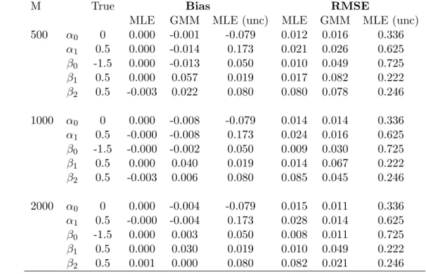
By setting ρ = 1, the weight that the quasi-likelihood puts on the auxiliary moments depends on the sample size.26 In that sense, our approach is similar to the GMM estimator proposed by Imbens and Lancaster (1994). However, the two estimators cannot be nested in any sense. The moment conditions in Imbens and Lancaster (1994) are not the same as the score of the quasi-likelihood defined in equation 15. When using a block-diagonal weighting matrix for each set of moment conditions, the GMM estimator minimizes the sum of the square of the scores minus a penalty function to account for the sum of square of the moment residual, while our estimator maximizes the sum the log-likelihood function minus the same quadratic penalty function. We have conducted a series of Monte Carlo simulations to analyze the small sample performance of both estimators, and found that our quasi-likelihood estimator performs equally well or better than GMM. These results are available in Appendix E. The appendix also provides additional details as to the differences between GMM and our quasi-likelihood approach.
Computation In order to evaluate the aggregate likelihood function, we must first solve the optimal initial offer defined implicitly by equation (6). This non-linear equation needs to be solved separately for every consumer/home-bank combination. We perform this operation numerically using a Newton algorithm that uses the first and second derivatives of firms’ expected profits. We use starting values defined as the expected initial quote from the complete information problem, for which we have an analytical expression. This procedure is robust and converges in a small number of steps. Notice that since the interior solution is additive in c, this equation needs to be solved only once for each evaluation of the likelihood contribution of each household,L(li, b(i)|Ii, h, θ). In addition, the integrals are evaluated numerically using a quadrature approximation.
6
Estimation results
6.1 Parameter estimates
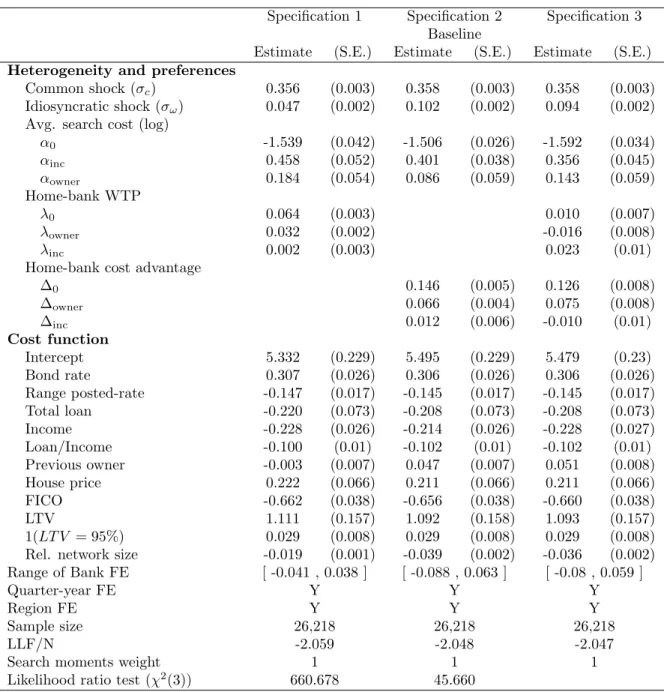
Table 2 summarizes the maximum-likelihood estimates from three specifications, each one varying the source of the loyalty advantage. In Specification (1), the loyalty advantage takes the form of a
WTP term, λ, for the home bank. In Specification (2), the home bank has a cost advantage, ∆, over competing lenders. Specification (3) nests both models.
Each specification implies that the home bank is more likely to “win” against rival banks at the competition stage, but have different implications for the price differences between loyal and switching borrowers. Holding fixed the magnitude of the idiosyncratic cost differences between lenders (σω), the WTP model implies a larger average price difference between loyal and switching borrowers, relative to the cost advantage model. This difference is relatively small in the data: loyal borrowers pay about 10 bps more than switching borrowers, or about 10% of the standard-deviation of residual rates. In Specification (1), the model reconciles these two features with small estimates ofσω and λ0. In contrast, the cost-advantage model leads to larger estimates of the differentiation
parameters, ∆ andσω. Also, the cost-advantage model fits the data significantly better.
We formally assess the performance of the two modeling choices by estimating Specification (3). The last row reports the results of two likelihood-ratio tests testing the null-hypothesis thatλi = 0 and ∆i = 0. We can easily reject the null hypothesis that the cost advantage parameters are zero; the test statistics is more than 40 times larger than the 1% critical value (i.e. 660.7 vs 16.3). In contrast, the null hypothesis of zero home-bank WTP parameters is much more modestly rejected (i.e. 45.7 vs 16.3).
A closer look at the estimates of λ in Specification (3) reveals that the intercept and owner
parameters are not significantly different from zero statistically or economically, while the estimated cost advantage parameters are large and precisely estimated. The reverse is true for the interaction of income and loyalty. This suggests that the relationship between loyalty and income is better explained by the WTP model. Still, the effect of income on the loyalty advantage is economically small and imprecise in all three specifications. Since the data do not support the WTP model, we use to the cost-advantage model as ourbaseline specification.
Table 11 in the Appendix, evaluates the robustness of the results to the weight assigned to the auxiliary search moments. Specifically, we re-estimated the model with weights of 0 and 100 on the auxiliary search moments. A weight of 100 is analogous to increasing the sample size of the search survey to be roughly on par with the number of observations in the mortgage contract data. Doing so tends to increase the magnitude and heterogeneity of the loyalty-advantage parameters (i.e λ
and ∆), and changes the sign of the income coefficient in the search cost function. This allows the model to better match the observed heterogeneity in the search probability across market-size and income groups (see goodness of fit discussion below).
across lenders is larger (e.g. σω = 0.12 instead ofσω = 0.1). Both features imply a larger predicted search probability in Specifications (4) and (5), relative to (2) and (3) (approximately 3 percentage points). The fact that these differences are fairly minor confirms that the model’s key parameters can be identified without using direct information on search behavior.
Next, we discuss the economic magnitude of the parameter estimates, focusing on the lending cost function and the search cost distribution. To better understand the magnitude of the estimates, recall that consumers choose a lender by minimizing their monthly payment net of the search cost. The monthly cost of supplying a $100,000 loan is a linear function of borrowers’ observed and unobserved characteristics, and the parameters are expressed in $100 per month. For instance, in Table 2 the variance parameter of the common shock, σc = 0.358, implies that the common lending-cost standard-deviation for a $100,000 loan with fixed attributes is equal to $35.80/month.
Lending cost function The first two parameters, σc and σω, measure the relative importance of consumer unobserved heterogeneity with respect to the cost of lending. The standard-deviation of the common component is 64% larger than the standard-deviation of idiosyncratic shock (i.e. 0.358 versus 0.128), suggesting that most of the residual price dispersion is due to consumer-level unobserved heterogeneity rather than to idiosyncratic differences across lenders.27
The estimate ofσωhas key implications for our understanding of the importance of market power in this market. Abstracting from systematic differences across banks, the average cost difference between the first- and second-lowest cost lender, c(1) and c(2), is equal to $20 in duopoly markets, $17 with three lenders, and approaches $14 whenN is equal 11.
In the model, market-power also arises because of systematic cost differences across banks: (i) bank fixed-effects, (ii) network size, and (iii) home-bank cost advantage. The estimates of the fixed-effects reveal relatively small differences across banks. Three of the eleven coefficients are not statistically different from zero (relative to the reference bank), and the range of fixed-effects is equal to $15/month in our baseline specification, or about the same scale as the standard-deviation of the idiosyncratic components.
We incorporate network size in the model by allowing the lending cost to depend on the relative branch network size of lenders in the same neighborhood. The estimates reveal that a lender with 3 times more branches than the average would experience a cost advantage of about $12/month (compared to a single-branch institution). This is consistent with our interpretation of the lend-ing cost function, as capturlend-ing elements of profits from complementary banklend-ing services that are increasing in branch-network size.
Turning to the estimate of ∆i, we find that the presence of the loyalty advantage corresponds to an average cost advantage of $17.10/month (for a loan size of $100,000). This cost advantage is substantial, given the fact thatσω is relatively small. At the estimated parameters, the probability that the home bank has a cost lower than the most efficient lender inNi is equal toG(1)(ωh) = 51%;
27The standard deviation of an extreme-value random variable is equal toσ
ωπ/
√