Game8 最近の更新履歴 yyasuda's website

(1)

166

CKWARD INDUCTION AND BGAME PERFECTION

T

o this point, our analysis of rational behavior has cent�red on the norm

_:

^l form-where we examine strategies and payof functIOns. Alth?ug

_�

^{t e} normal-form concepts are valid for evey game (because a� e:tensIve orm can be translated into the normal form), they are most convmcmg f�r games _. h' h all of the players' decisions are made simultaneously �nd llldep�n m w IC

.

_.

_f

d narruc propertIes d tl I want you to now consider games wIth mteres mg y , w

e

:

^er

�

^'the extensive form more precisely captures the order of moves and the

information structure. _. _. _.

. n of the To see that there are some interestmg Issues regrdI�g comparlso normal and extensive forms, study the game pictured m FIgure

)

15

_;

. Th_.ere are two irms in this market game: a potential entrant (player ¹ ^an_.^{an mcu}

�

bent (player 2). The entrant decides whether or not to enter the mcum

_:

^ent

_�

industr If the entrant stays out, then the incumbent gets � large pro t an the en

_� _�

nt gets zero. If the potential entrant does e?ter th� mdustr

_i i _� _:

ⁿ

fi

^� ^�

incumbent must choose whether or not to engage m a pnce war. ^t

. . d

ar then both irms sufer. If the incumbent accommo ates trIg"ers a pnce w ,

the

_:

ntrant, then they both obtain modest proit�.

_.

Pictured in Figure ^15.1are both the extensIve- and the nOlmal-f?rm rep _

resentations of this market game. A quick look at the n.ormal form wIll reveal that the game has two Nash equilibria (in pure strategIes):. (I, A) and ^(0,^P

^!

_� 'l'b . m should not strike you as controversial. The latter eqUl The former eqUl I nu

FIGURE 15.1 Entry and predation.

Out ^0,4

�2'2

�-l'-I

1 2

I 0

A P

2,2

^{-I, -I}

0,4 0,4

•

Sequential Rationality and Backward Induction 167

librium calls for an explanation. With the extensive form in mind, equilibrium

(0, P) has the following interpretation. Suppose the players do not select their strategies in real time (as the game progresses), but rather choose their strate gies in advance of playing the game. Perhaps they write their strategies on slips of paper, as instructions to their managers regarding how to behave. The entrant prefers not to enter if she expects the incumbent to initiate a price war. That is, she responds to the threat that player 2 will trigger a price war in the event that player 1 enters the industry. For his part, the incumbent has no in centive to deviate from the price-war strategy when he is convinced that the entrant will stay out. Note that the incumbent's thought process here consists of an ex ante evaluation; that is, the incumbent is willing to plan on playing the price-war strategy when he believes that his decision node will not be reached. Is the (0, P) equilibrium really plausible? Many theorists think not, be cause games are rarely played by scribbling strategies on paper and ignoring the real-time dimension. In reality, player 2's threat to initiate a price war is incredible. Even if player 2 plans on adopting this strategy, would he actually carry it out in the event that his decision node is reached? He would prob ably step back for a moment and say, "Whoa, Penelope! I didn't think this information set would be reached. But given that this decision really counts now, perhaps a price war is not such a good idea after all." The incumbent will therefore accommodate the entrant. Furthermore, the entrant ought to think ahead to this eventuality. Even though the incumbent may "talk tough," claim ing that he will initiate a price war if entry occurs, the entrant understands that such oehavior would not be rational when the decision has to be made. Thus, the potential entrant can enter the industry with conidence, nowing that the incumbent will capitulate. ^IThere are many examples of games such as these, where an equilibrium speciies an action that is irrational, conditional on a partiCUlar information set being reached. Not all of the examples concen incredible threats. You might lip through preceding chapters and search for such games.

SEQUENTIAL RATIONALITY AND BACKWARD INDUCTION

As the example in Figure 15.1 indicates, more should be assumed about play ers than that they select best responses ex ante (from the point of view of the

I Children sometimes play games like these with their parents. Parents may threaten to withhold a trip to the ice·cream parlor, unless a child eats his vegetables. But the parents may have an independent interest in going to the ice-cream parlor and, if they go, then they will have to take the child with them, lest he be left at home alone. They can punish the child by skipping sundaes, but they would also be punishing themselves in the process. _A

shrewd child knows when his parents do not have the incentive to carry out punishments; such children grow up to be economists or attorneys. They also feed peas to their dogs from time to time.

(2)

168 15: Backward Induction and 5ubgame Perfection

beginning of the game). Players ought to demonstrate rat

_�

onali

_�

w

_�

enever they are called on to make decisions. This is called sequentwl ratlOnalzty.

Sequential rationality: An optimal strategy for a play_�r shoul

_�

max imize his or her expected payof, conditional on every mformatlOn set at which this player has the move. That is, player i's strategy should specify an optimal action from each of player i's i?formation se

_�

s, even those that player i does not believe (ex ante) wIll be reacl;1ed m the game.

If sequential rationality is common knowledge between the

.players (at every information set), then each player will "look ahead" to con_�lder wh_�t players will do in the future in response to her move at a particular mformatlOn set.

To determine the strategies that are consistent with the common knowl edge of sequential rationality, we evaluate whether each strateg

_�

is _co�dition ally dominated. A strategy Si for player i is conditi

_�

nally

_�

ommated If, con tingent on reaching some information set of player .z.� there IS an_�ther strategy

J that strictly dominates it. One can remove condltlOnally dommated strate g

_i

es by using an iterated procedure that is roughl_�s

_�

milar to the procedure for normal-form games. However, a complete descnptlOn of the procedure re quires more analysis than is appropriate herein. 2 It is mo_�e wort

.hwhile to focus on a simpler version of doinance known as bacward znductlOn.

Backward induction: This is the process of analyzing a game from . back to front (from information sets at the end of the tree to informa tions sets at the beginning). At each information set, one strikes from consideration actions that are dominated, given the terminal nodes that can be reached.

To determine the optimal action at an information set, one must lo_�k ah_�ad in the game. Thus, the easiest information sets at which to evalu

.^{ate raU}^?nallty are those at the end of the tree-that is, those whose nodes are ImmedIate prede cessors of terminal nodes. When the optimal actions have been determine

_�

for these information sets, one can move to immediate predecessors and contmue the process until the initial node is reached. _. _.

Backward induction can be tricky for games of Imperfect InformatlOn, .

where it is best to use the full-blown conditional-dominance concept that is not introduced here. (Such games are addressed later in this chapter in the context of equilibrium. ) For now, consider the class of exte_�sive-form ga_�es with perfect information. Each game in this class can be eaSIly analyzed usmg backward induction. If there are no ties in the payofs-where two or more

2Conditional dominance is deined and studied in _M.Shimoji and _1.Watson, "Conditional Dominance, Ra-• tionalizability, and Game Forms," Joul7lal of Economic TheO/y 83(1998): 161-195.

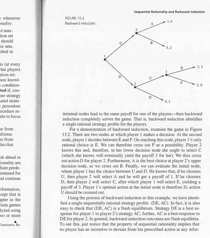
FIGURE 15.2 Backward induction.

?

u

D

Sequential Rationality and Backward Induction 1,4

5,2

�3,3

-� 2'O

6,2

terminal nodes lead to the same payof for one of the players-then backward induction completely solves the game. That is, backward induction identiies a single rational strategy profile for the players.

For a demonstration of backward induction, examine the game in Figure 15.2. There are two nodes at which player 1 makes a decision. At the second node, player 1 decides between E and . On reaching this node, player 1's only rational choice is E. We can therefore cross out F as a possibility. Player 2 knows this and, therefore, in her lower decision node she ought to select C (which she knows will eventually yield the payof 3 for her). We thus cross out action D for player 2. Furthermore, A is the best choice at player 2's upper decision node, so we cross out B. Finally, we can evaluate the initial node, where player 1 has the choice between U and D. He knows that, if he chooses U, then player 2 will select A and he will get a payoff of 1. If he chooses D, then player 2 will select C, after which player 1 will select E, yielding a payof of 3. Player 1's optimal action at the initial node is therefore D; action U should be crossed out.

Using the process of backward induction in this example, we have identi ied a single sequentially rational strategy proile: (DE, AC) . In fact, it is also easy to check that (DE, AC) is a Nash equilibrium. Strategy DE is a best re sponse for player 1 to player 2's strategy AC; further, AC is a best response to DE for player 2. In general, backward-induction outcomes are Nash equilibria. To see this, just notice that the property of sequential rationality implies that no player has an incentive to deviate from his prescribed action at any in for-

169

(3)

170 15: Backward Induction and Subgame Perfection

mation set. Further, because every inite game with perfect information can be solved by backward induction, every such game has a Nash equilibrium.

Result: Every in�te game with perfect information has a pure-strategy Nash equilibrium. Backward induction identiies an equilibrium.3 If there are ties in the payoffs, then there may be more than one such equilib rium and there may be more than one sequentially rational strategy profile.

SUBGAME PERFECTION

The concept of backward induction can be expanded to cover general extensive form games. One way of doing this is to think of a sequential version of rationalizability, where players must play best responses to their beliefs at all information sets. Such a notion has been developed and is related to the conditional-dominance concept, but, as with conditional dominance, it is a bit too technical to present here.4 Instead, I focus on 'equilibrium and deine a reinement of Nash's concept that incorporates sequential rationality. Versions of this kind of refinement are identified by the term "perfection."

The concept of subgame pefection starts with a description of a subgame. Given an extensive-form game, a node ^xin the tree is said to initiate a sub game if neither ^xnor any of its successors are in an information set that contains nodes that are not successors of ^x.A subgame is the tree structure deined by such a node x and its successors.

This deinition may seem complicated on irst sight, but it is not dificult to understand. Take any node ^xin an extensive form. Examine the collection of. nodes given by x and its successors. If there is a node y that is not a succes sor of x but is connected to x or one of its successors by a dashed line, then

x does not initiate a subgame. In other words, once players are inside a sub game, it is common knowledge between them that they are inside it. Subgames are self-contained extensive forms-meaningful trees on their own. Subgames that start from nodes other than the initial node are called proper subgames. Observe that, in a game of perfect information, evey node initiates a subgame.

3H. . Kuhn, "Extensive Games and the Problem of Information," in ComribUlions to the Theory o/Games,

vol. II (Annals 0/ Mathematics Studies, 28), ed. H . W. Kuhn and A. W. Tucker (Princeton, NJ: Princeton University Press, 1953), pp. 193-216.

4Extensive-form rationalizability was introduced in D. Pearce, "Rationalizable Strategic Behavior and the Problem of Perfection," Econometrica 52(1984):1029-1050. It was clariied by P. Battigalli, "On Rationaliz ability in Extensive Games," Journal 0/ Economic Theory 74( 1997):40-61. The relation to conditional domi nance is reported in M. Shimoji and J. Watson, "Conditional Dominance, Rationalizability, and Game Forms,"

Journal 0/ Economic Theory 83(1998): 161-195.

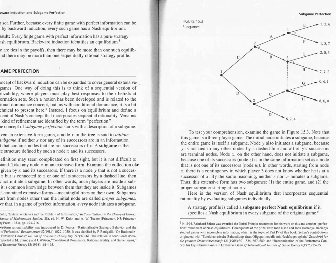
FIGURE 15.3 Subgames.

u

D

Subgame Perfection

�

^2'O"

!�

^:_I ^7,7,2

�;

I w ^G ^0,6,1

H _8,6,0

6,2,4

To test your comprehension, examine the game in Figure 15.3. Note that this game is a three-player game. The initial node initiates a subgame, becaise the entire game is itself a subgame. Node y also initiates a subgame, because y is not tied to any other nodes by a dashed line and all of y's successors are terminal nodes. Node ^x,on the other hand, does not initiate a subgame, because one of its successors (node z) is in the same information set as a node that is not one of its successors (node w). In other words, starting from node

x, there is a contingency in which player 3 does not know whether he is at a successor of ^x.By the same reasoning, neither z nor w initiates a subgame. Thus, this extensive form has two subgames: (1) the entire game, and (2) the proper subgame starting at node y.

Here is the version of Nash equilibrium that incorporates sequential rationality by evaluating subgames individually.

A strategy proile is called a sub game perfect Nash equilibrium if it speciies a Nash equilibrium in every subgame of the original game.s

5In 1994, Reinhard Selten was awarded the Nobel Prize in ec_�nomics for his work on this and another "perfec tion" reinement of Nash equilibrium. Corecipients of the prize were John Nash and John Harsanyi. Harsanyi studied games wilh incomplete information, which is the topic of Part IV of this book. Selten's contributions originated with "Spieltheoretische Behandlung eines Oligopolmodells mit Nachfragetragheit," Zeitschrir fur die gesamte S/aa/sV;ssenscha/t 121(1965):301-324,667-689, and "Reexamination of the Perfectness Con cept for Equilibrium Points in Extensive Games," Intenat;onal Journal o/Game TheY 4(1975):25-55.

171

(4)

172 15: Backward Induction and Subgame Perfection FIGURE 15.4

Subgame perfection.

1 ²

_UA

UB DA DB U

X

3,4 2,1

2,6 2,6

Y ¹

2,0 1,4

2,6 2,6

:3,4

: y

_1,4

�2'1

I

Y

2,0

2

^X ^Y

A

3,4 1,4

B

2,1

^•

2, 0

The basic idea behind subgame perfection is that a solution concept should be consistent with its own application from anywhere in the game where it can be applied. Because Nash equilibrium can be applied to well-defined extensive form games, subgame perfect Nash equilibrium requires the Nash condition to hold on all subgames.

To understand how to work with the concept of subgame perfection, con sider the game pictured in Figure 15.4. Note irst that this game has one proper subgame, which starts at the node reached when player 1 plays V at the initial node. Thus, there are two subgames to evaluate: the proper sub game as well as the entire game. Because strategy proiles tell us what the players do at every information set, each strategy proile speciies behavior in the proper subgame even if this sub game would not be reached. For example, consider strategy proile (DA, X). If this profile is played, then play never enters the proper sub game. But (DA, X) does include a speciication of what the players would do conditional on reaching the proper subgame; in particular, it prescribes action A for player 1 and action X for player 2.

Continuing with the example, observe that two normal-form games appear next to the extensive form in Figure 15.4. The irst is the normal-form version

Subgame Perfection

of the entire extensive form, whereas the second is the normal-form version of the proper subgame. The former reveals the Nash equilibria of the entire game; we examine the latter to find the Nash equilibria Of the proper subgame. In the entire game, (VA, X), (DA, Y), and (DB, Y) are the Nash equi libria. But not all of these strategy profiles are subgame perfect. To see this, observe that the proper subgame has only one Nash equilibrium, (A, X). The strategies (DA, Y) and (DB^,Y) are not sub game perfect, because they do not specify Nash equilibria in the proper subgame. In particular, (DA, Y) stipu lates that (A, Y) be played in the proper subgame, yet (A, Y) is not an equi librium. Furthermore, (DB, Y) specifies that (B, Y) be played in the subgame, yet (B, Y) is not an equilibrium. Thus, there is a single subgame perfect Nash equilibrium in this example: (VA, X).

The subgame perfection concept requires weak congruity at every sub game, meaning that, if any particular subgame is reached, then we can expect the players to follow through with the prescription of the strategy. This is an important consideration, whether or not a given equilibrium actually reaches the subgame in question. The example in Figure 15.4 illustrates this point vividly. Nash equilibrium (DA, Y) entails a kind of threat that the players jointly make to give player 1 the incentive to select D at his irst information set. But the threat is not legitimate. In the proper subgame, (A, Y) is about as stable as potassium in water. Player 1 has the strict incentive to deviate from this prescription.6

Several facts are worth noting at this point. First, and most obvious, rec ognize that a subgame perfect Nash equilibrium is a Nash equilibrium because such a profile must specify a Nash equilibrium in every subgame, one of which is the entire game. We thus speak of subgame perfection as a reinement of Nash equilibrium. Second, for games of perfect information, backward induc tion yields subgame perfect equilibria. Third, on the matter of inding sub game perfect equilibria, the procedure just described is useful for many inite games. One should examine the matrices corresponding to all of the subgames and lo cate Nash equilibria. For ininite games and for mixed equilibria, it is often easier to start with the subgames that are toward the end of the extensive form, with the hope that these subgames have unique Nash equilibria. Then one can work backward by embedding these equilibrium outcomes into the "larger"

6Th at player 2 is indiferent between _{CA, X)}and _{CA, Y)}in the proper subgame implies a very diferent con clusion using the notion of conditional dominance. In the proper subgame, aIthough player I's action B is stricken, neither of player 2's actions are dominated. Thus, player I could rationally play _DAwith the belief that player 2 selects strategy _.The difference between subgame perfect Nash equilibrium and conditional dominance is therefore due to the fact that proile _{CA, Y)}is rationalizable, yet it is not a Nash equilibrium, in the proper subgame.

173

(5)

subgames. This procedure is illustrated in the following guided exercise and, more generally, in Chapter 16.

GUIDED EXERCISE

Problem: Consider the ultimatum bargaining game described at the end of Chapter 14. In this game, the players negotiate over the price of a painting that· player 1 can sell to player 2. Player 1 proposes a price p to player 2. Then, after observing player l's offer, player 2 decides whether to accept it (yes) or reject it (no). If player 2 accepts the proposal, then player 1 obtains p and player 2 obtains 100 -_p.If player 2 rejects the proposal, then each player gets zero. Verify that there is a subgame perfect Nash equilibrium in which player 1

ofers p* ⁼100 and player 2 has the strategy of accepting any offer p :: 100

and rejecting any ofer p ^>100. ^.

Solution: The exercise here is to verify that a particular strategy profile is a subgame perfect equilibrium. We do not have to determine all of the subgame perfect equilibria. Note that there is an infinite number of information sets for player 2, one for each possible ofer of player 1. Each one of these information sets consists of a single node and initiates a simple subgame in which player 2 says "yes" or "no" and the game ends. The suggested strategy for player 2, which accepts (says "yes") if and only if p ^{:: 100,}implies an equilibrium in every such subgame. To see this, realize that player 2 obtains a payoff of

100 -_pif he accepts, whereas he receives 0 if he rejects, so accepting is a best response in every subgame with p :: 100; rejecting the ofer is a best response in every subgame with p : 100. For p ⁼ 100, both accepting and rejecting are best responses; thus, player 2 is indiferent between accepting and rejecting when p ⁼ ^100.We are assuming that, in this case of indiference, player 2 accepts.

Having veriied that player 2 is using a sequentially rational strategy, which implies equilibrium in every proper subgame, let us turn to the entire ultimatum game (from the initial node) and player l's incentives. Observe that the ofer p* ⁼¹⁰⁰is a best response for player 1 to the strategy of player 2. If player 1 offers this price then, given player 2's strategy, player 2 will accept it and player l's payoff would be 100. On the other hand, if player 1 were to ofer a higher price, then player 2 would reject it and player 1 would get a payof of zero. Furthermore, if player 1 were to offer a lower price p ^<100,

then player 2 would accept it and player 1 would obtain a payof of only p.

Also note that, in the entire game, player 2's strategy is a best response to player l's strategy of offering p* ⁼100, because player 2 accepts this offer.

Exercises

We have thus established that the suggested strategy profile induces a Nash equilibrium in all of the subgames, including the entire game, and so we have a subgame perfect Nash equilibrium. You will ind further analysis of the ulti matum bargaining game in Chapter 19, where it is shown that the equilibrium we have just identified is, in fact, the unique subgame perfect equilibrium.

EXERCISES

1. Consider the following extensive-form games.

B

A

(a) _2,6

A

B

(b)

2

_---

_D _F

2,3

c

1,4

D

F

E

1,5

�4'O

� 8'3

175

(6)

2

(c)

---o

2,2,2

B c

4,3,1

�3,2,1

3

^I_I

.

: Y 5, 0, 0

I I

:26

" _7,5,5

Solve the games by using backward induction.

2. Compute the Nash equilibria and subgame perfect equilibria for the follow ing games. Do so by writing the normal-form matrices for each game and its subgames. Which Nash equilibria are not subgame perfect?

w

z c

2 (a) D

�30 �

^I ^8'5

:',6

y

2,1

6,4

3,2

u

D

(b)

3. Consider the following game.

B

c

D

Exercises

2,3

5,4

� ₆ ₂

^'

� _2,6

0,2

177

E

^�2"

2

^C

<=<:::

B ^J

5,4 4,5

(a) Solve the game by backward induction and report the strategy profile that results.

(b) How many proper subgames does this game have?

4. Calculate and report the subgame perfect Nash equilibrium of the game de scribed in Exercise 3 in Chapter 14.

Game8 最近の更新履歴 yyasuda's website

T

:

�

.

:

�

;

�

:

�

� �

i i � :

� �

:

.

!

�2'2

�-l'-I

2,2

�

�

�

�

�

�

�

�

i

�

�

5,2

�3,3

-� 2'O

6,2

�

!�

�;

1 2

3,4 2,1

2,6 2,6

2,0 1,4

2,6 2,6

:3,4

1,4

�2'1

2,0

2

3,4 1,4

2,1

2, 0

---

2,3

1,4

1,5

�4'O

� 8'3

2

2,2,2

4,3,1

�3,2,1

3

.

:26

�30 �

:',6

2,1

6,4

3,2

2,3

� 6 2

� 2,6

0,2

�2"

2

<=<:::

5,4 4,5

_:

_�

_.

_;

_:

_�

_� _�

_i i _� _:

^� ^�

_:

_.

^!

_�

_�

_�

_�

_�

_�

_�

_�

_i

_�

_�

1 ²

_1,4

_---

� ₆ ₂

� _2,6

^�2"