Article
A Stochastic Programming Approach with Improved
Multi-Criteria Scenario-Based Solution Method for
Sustainable Reverse Logistics Design of Waste
Electrical and Electronic Equipment (WEEE)
Hao Yu * and Wei Deng Solvang
Department of Industrial Engineering, Faculty of Engineering Science and Technology, UiT—The Arctic University of Norway, Narvik 8505, Norway; [email protected]
* Correspondence: [email protected]; Tel.: +47-7696-6328
Academic Editor: Vincenzo Torretta
Received: 30 October 2016; Accepted: 13 December 2016; Published: 17 December 2016
Abstract:Today, the increased public concern about sustainable development and more stringent environmental regulations have become important driving forces for value recovery from end-of-life and end-of use products through reverse logistics. Waste electrical and electronic equipment (WEEE) contains both valuable components that need to be recycled and hazardous substances that have to be properly treated or disposed of, so the design of a reverse logistics system for sustainable treatment of WEEE is of paramount importance. This paper presents a stochastic mixed integer programming model for designing and planning a generic multi-source, multi-echelon, capacitated, and sustainable reverse logistics network for WEEE management under uncertainty. The model takes into account both economic efficiency and environmental impacts in decision-making, and the environmental impacts are evaluated in terms of carbon emissions. A multi-criteria two-stage scenario-based solution method is employed and further developed in this study for generating the optimal solution for the stochastic optimization problem. The proposed model and solution method are validated through a numerical experiment and sensitivity analyses presented later in this paper, and an analysis of the results is also given to provide a deep managerial insight into the application of the proposed stochastic optimization model.
Keywords: WEEE; reverse logistics; stochastic optimization; mixed integer programming; scenario-based solution; sustainable development; carbon emissions
1. Introduction
Today, with rapid technological advancement and economic development, the manufacturing of electrical and electronic products has become one of the most rapidly developing and growing industries [1–3]. This growth has significantly altered the lifestyle and consumption pattern of human beings [2,4]. On the one hand, more and more innovative, well-designed, and multi-functional electrical and electronic products are introduced, usually at an attractive price, to make our lives better and more convenient. On the other hand, customers’ pursuit of a better lifestyle also leads to an increasingly shortened product life cycle, particularly for electrical and electronic products, which results in rapidly increased generation of Waste Electrical and Electronic Equipment (WEEE) all over the globe. The annual increase of WEEE generation has reached approximately 5% since 2005 [5], which is almost three times higher than the increase of other waste [6]. In 2012, the WEEE generation in the world is approximately 49 million metric tons [7], and the three largest markets for electrical and electronic products (the United States, China, and the European Union) together contribute 54.1% of the total amount of WEEE generation [7]. The rapid growth of WEEE generation has become a significant
challenge due to the lack of formal recycling and recovery channels [8], and an earlier study has revealed that only 1.5 million metric tons of WEEE in Europe were recycled through formal take-back schemes [4]. A recent report released by the Countering WEEE Illegal Trade (CWIT) project [9] reveals that the total amount of WEEE generated in Europe was 9.45 million tons in 2012, of which only 35% was recycled and treated through the formal recycling system; the other 65% was exported (15.8%), recycled through non-compliant conditions in Europe (33.4%), scavenged for valuable parts (7.9%), or sent to landfill (7.9%). According to the report [9], due to the mismanagement of discarded electronics in Europe, there is still a large amount of WEEE sent to and recycled in developing countries, e.g., China, Vietnam, etc., where, unlike in developed countries, most of the WEEE are reused and recycled under lower standards through low-tech companies or disposed of in landfills [10]. From a global perspective, this will reduce the economic sustainability (waste of recyclable and valuable resources [9]), environmental sustainability (environmental pollution [9]), as well as social sustainability (risk to workers’ health [9,11]) of modern society. Therefore, more effort should be directed to providing guidelines and support systems for decision-makers in order to enhance formal recycling systems for sustainable management of WEEE, so more WEEE can be recycled and treated in an economically efficient, environmentally sound, and socially responsible manner.
Reverse logistics is considered as one of the most effective solutions for value recovery from end-of-life and end-of-use products [12]. Reverse logistics is defined as the process starting from the customer towards the raw material supplier, and it aims at—through planning, operating, and managing efficient material flow, information flow, and cash flow—recovering the remaining value from end-of-life and end-of-use products and disposing of waste in a proper way [13]. Due to public concern about sustainable development, reverse logistics activities have been extensively focused in the past two decades [14–17]. Compared with other used products, the reverse logistics design for WEEE management is more complicated, because WEEE contains not only renewable materials and components, e.g., glass, plastics, and precious metals [8], which need to be reused and recycled, but also hazardous substances, e.g., nickel, lead, and mercury [18,19], which have to be properly treated or disposed of in order to minimize the risk to people’s health and the environment. Therefore, the development of advanced tools for complex decision-making problems related to the design and planning of a sustainable reverse logistics system for WEEE is of paramount importance.
In order to have an overview of the theoretical development and practical implementation, this paper reviews some of previous studies regarding the reverse logistics of WEEE, and an extensive literature review of the decision models of WEEE management is provided by Xavier and Adenso-Diaz [20]. Walther and Spengler [21] formulate a linear programming for allocating WEEE to different facilities in an optimal fashion, and the model is used to estimate the influence of EU WEEE Directive on reverse logistics in Germany. Dat et al. [22] introduce a mixed integer programming for minimizing the total costs of reverse logistics of WEEE, considering the costs of collection, transportation, treatment, and income from the sale of recycled products. Gomes et al. [23] develop a generic mixed integer program for multi-product reverse logistics network design of WEEE; the model determines the best locations of collection and sorting centers and the material flows in each route.
Grunow and Gobbi [27] develop a decision support model for assigning different municipalities to different waste management schemes in an efficient and fair manner. Achillas et al. [4] formulate a location–allocation model for regulators and policy-makers for the optimal design of reverse logistics network of WEEE. Capraz et al. [28] propose a mixed integer linear programming for decision-making of recycling companies of WEEE, and the model simultaneously determines the maximal bid price offered by the company and the optimal operational plan of the plant. Liu et al. [29] propose a quality-based price competition model for assessing the performance of both formal and informal recycling channels of WEEE. The study reveals that the quality is the most important influencing factor for WEEE recycling, and high-quality WEEE are preferred by both formal and informal markets. Furthermore, the informal recycling market is of great advantage when the quality of WEEE is high and the formal recycling channel is not heavily subsidized by the government.
Manzini and Bortolini [30] introduce a two-stage decision-aided system for both strategic and operational decision-making of reverse logistics of WEEE. The optimal location–allocation plan is first determined by a mixed integer programming, and a heuristic algorithm is then applied to solve the vehicle routing problem. Yao et al. [31] develop a quadratic optimization model to determine the minimum number of transit sites for reverse logistics of WEEE, and a modified ant colony algorithm is then applied for routing the collection vehicles. Tsai and Hung [32] propose a two-stage decision framework for planning a treatment and recycling system for WEEE. The waste treatment companies are first selected at the treatment stage, and a linear programming is formulated in recycling stage for maximizing the profit generated from WEEE recycling. Mar-Ortiz et al. [33] formulate an integer programming model for the vehicle routing problem of WEEE, and two computational algorithms, a GRASP-based algorithm and a saving-based algorithm, are employed and compared in resolving the complex optimization problem.
Shokohyar and Mansour [34] develop a simulation- and optimization-based framework for sustainable planning of the reverse logistics network of WEEE. Different network configurations are first tested in the simulation stage through the professional simulation software Arena, and then, in the optimization stage, a multi-objective model is formulated to determine the value of three objective functions: profit, environmental influence, and social sustainability. Yu and Solvang [2] formulate a bi-objective mixed integer programming for sustainable reverse logistics design of WEEE. The model simultaneously balances the overall system costs and carbon emissions, and the two objective functions are combined with the weighted sum method.
The remainder of the paper is organized as follows. Section2provides the problem statement and formulates the stochastic mixed integer programming for the design of a sustainable reverse logistics system for WEEE management under uncertainty. Section3introduces the two-stage multi-criteria scenario-based solution method for stochastic optimization problem, and the difference between the improved solution method and the original solution method is presented in this section. Section4 presents a numerical experiment in order to illustrate the application of the proposed model in the decision-making of reverse logistics system design of WEEE. Section5provides sensitivity analyses in order to validate the model with changing parameters. Section6concludes the paper and provides suggestions for future research.
2. Problem Statement and Modeling
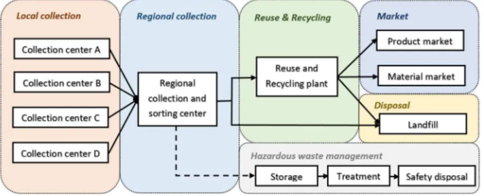
Figure1illustrates the reverse logistics system for WEEE management. The end-of-use and end-of-life electrical and electronic products are first collected at a local WEEE collection center (e.g., retailers of electronic products, supermarkets, public facilities for WEEE collection, etc.), and then will be transported to a regional collection center for preprocessing. At the regional collection center, WEEE are inspected and sorted for further treatment including reuse, recycling, and disposal. It is noteworthy that some electrical and electronic products contain hazardous materials that have to be separated out at this step and sent to specialized hazardous waste treatment plants. The recyclable parts and components from WEEE are sent for reuse and recycling, and the non-recyclable fraction is sent to an incineration plant or a landfill for proper disposal. The recycled products from WEEE will be sold at primary or secondary markets, and the recycled components will be sold to manufacturers of electrical and electronic products for material recovery.
Figure 1.Reverse logistics system for WEEE management.
The proposed mathematical model aims at determining the optimal configuration of the reverse logistics system for WEEE, which includes the locations of regional collection centers and recycling plants, and the material flows between different facilities. Due to the uncertainty, the generation of WEEE, price of recycled products, and price of recycled materials are considered to be stochastic parameters, and the different sources of WEEE and the environmental influence are also taken into account in this model. Therefore, the proposed model is a multi-source, multi-echelon, and capacitated stochastic network optimization problem. In this paper, we use the word “product” to differentiate the sources of WEEE.
The assumptions of the model are given as follows:
• The number and locations of local collection centers, product markets, material markets, and disposal facilities are known.
• The potential locations of regional collection centers and recycling plants are known.
• The fixed costs, unit transportation costs, and unit processing costs are known.
• The WEEE can be converted at a fixed rate to new products, recycled parts, disposal fractions, and hazardous materials.
• The carbon emissions rate is mainly determined by the size of facility and technology adopted in the treatment and transportation of WEEE.
The sets, parameters, and decision variables are given as follows:
Sets:
C Set of local collection sites of WEEE, indexed byc
R Set of potential locations of regional collection centers of WEEE, indexed byr P Set of potential locations of recycling plants of WEEE, indexed byp
H Set of hazardous waste management systems, indexed byh F Set of product market, indexed byf
M Set of material market, indexed bym D Set of disposal sites, indexed byd L Set of products, indexed byl S Set of scenarios, indexed bys
Parameters:
Fxr Fixed cost of opening regional collection center at potential locationr∈R
Fxp Fixed cost of opening recycling plant at potential locationp∈P
Cprl Unit cost at regional collection centerr∈Rfor processing productl∈L
Cppl Unit cost at recycling plantp∈Pfor processing productl∈L
Cpd Unit cost at disposal sited∈D
Cph Unit cost at hazardous waste management systemh∈H
PCpsf l Unit price of recycled productl∈Lat product marketf∈Fin scenarios∈S PCmsml Unit price of recycled productl∈Lat material marketm∈Min scenarios∈S
Ctrlcr Transportation cost per unit productl
∈Lfrom local collection sitec∈Cto regional collection centerr∈R
Ctrlrp Transportation cost per unit recyclable fraction of productl∈Lfrom regional collection siter∈Rto recycling plantp∈P
Ctrlrd Transportation cost per unit disposed fraction of productl
∈Lfrom regional collection centerr∈Rto disposal sited∈D
Ctrlrh Transportation cost per unit hazardous fraction of productl∈Lfrom regional collection centerr∈Rto hazardous waste management systemh∈H
Ctrl p f Transportation cost per unit recycled fraction of productl
∈Lfrom recycling plantp∈Pto product marketf∈F
Ctrl pm Transportation cost per unit recycled fraction of productl
∈Lfrom recycling plantp∈Pto material marketm∈M
Ctrl pd Transportation cost per unit disposed fraction of productl
∈Lfrom recycling plantp∈Pto disposal sited∈D
θ Unit cost of carbon credit
COcap2 Carbon emissions cap for reverse logistics system for WEEE
Cols
lc Amount of productl∈Lcollected at local collection sitec∈Cin scenarios∈S
Capacityrl Capacity of regional collection centerr∈Rfor productl∈L
Capacitypl Capacity of recycling products centerp∈Pfor productl∈L
ϕl p Recycling fraction of productl∈L
ϕld Disposed fraction of productl∈L
ϕlh Hazardous fraction of productl∈L
Lm′ An infinitely large positive number
ϑl f Conversion rate of productionl∈Lto product marketf∈F
ϑlm Conversion rate of productionl∈Lto material marketm∈M
ϑld Conversion rate of productionl∈Lto disposal sited∈D
Emsp Carbon emissions per unit capacity for opening a recycling plantp∈P
Emslcr
Carbon emissions for transporting one unit productl∈Lfrom local collection sitec∈Cto regional collection centerr∈R
Emslrp Transportation cost one unit recyclable fraction of product
l∈Lfrom regional collection site
r∈Rto recycling plantp∈P
Emslrd
Transportation cost one unit disposed fraction of productl∈Lfrom regional collection center
r∈Rto disposal sited∈D
Emslrh
Transportation cost one unit hazardous fraction of productl∈Lfrom regional collection center
r∈Rto hazardous waste management systemh∈H
Emsl p f Transportation cost one unit recycled fraction of product
l∈Lfrom recycling plantp∈Pto product marketf∈F
Emsl pm
Transportation cost one unit recycled fraction of productl∈Lfrom recycling plantp∈Pto material marketm∈M
Emsl pd
Transportation cost one unit disposed fraction of productl∈Lfrom recycling plantp∈Pto disposal sited∈D
Decision variables (First-level):
Ys r =
( 1 0
Potential location of regional collection centerr∈Ris selected in scenarios∈S
Otherwise
Yps= (
1 0
Potential location of recycling plantp∈Pis selected in scenarios∈S
Otherwise Decision variables (Second-level):
Qgrls Amount of productl∈Lprocessed at regional collection centerr∈Rin scenarios∈S Qgspl Amount of recycled fraction of productl∈Lprocessed at recycling plantp∈Pin scenarios∈S Qgsd Amount of disposed fraction of productl∈Lprocessed at disposal sited∈Din scenarios∈S
Qgsh Amount of hazardous fraction of productl∈Lprocessed at hazardous waste management
systemh∈Hin scenarios∈S Qgs
f l Amount of recycled fraction of productl∈Lsold at product marketf∈Fin scenarios∈S Qgsml Amount of recycled fraction of productl∈Lsold at material marketm∈Min scenarios∈S
Qtrs lcr
Amount of productl∈Ltransported from local collection sitec∈Cto regional collection centerr∈Rin scenarios∈S
Qtrslrp Amount recycled fraction of productl∈Ltransported from regional collection siter∈Rto
recycling plantp∈Pin scenarios∈S
Qtrslrd Amount of disposed fraction of productl∈Ltransported from regional collection centerr∈R
to disposal sited∈Din scenarios∈S
Qtrs lrh
Amount of hazardous fraction of productl∈Ltransported from regional collection center
r∈Rto hazardous waste management systemh∈Hin scenarios∈S
Qtrsl p f Amount of recycled fraction of productl∈Ltransported from recycling plantp∈Pto product
marketf∈Fin scenarios∈S
Qtrsl pm Amount of recycled fraction of productl∈Ltransported from recycling plantp∈Pto material
marketm∈Min scenarios∈S
Qtrs l pd
Amount of disposed fraction productl∈Ltransported from recycling plantp∈Pto disposal sited∈Din scenarios∈S
COS
2 Total amount of carbon emissions from the reverse logistics system for WEEE
emissions of the reverse logistics activities for WEEE management are quantified by a well-established method: carbon trading [39,40] and combined with the cost objective. Furthermore, it is noteworthy that the model aims at determining the optimal and most reliable and robust solution through all possible scenarios in the reverse logistics design of WEEE.
Min cost=
∑
r∈R
FxrYrs+ ∑ l∈L
∑
r∈R
CprlQpsrl
+ (
∑
p∈P
FxpYrp+ ∑ l∈L
∑
p∈P
CpplQgspl )
+
∑
d∈D
CpdQgsd+ ∑ h∈H
CphQgsh
− (
∑
f∈F PCps
f lQgsf l+ ∑ m∈M
PCms mlQgsml
)
+
∑
l∈L
∑
c∈C
∑
r∈R
CtrlcrQtrs lcr
+ (
∑
l∈L
∑
r∈R
∑
p∈P
CtrlrpQtrslrp+∑ l∈L
∑
r∈R
∑
d∈D
CtrlrdQtrslrd+ ∑ l∈L
∑
r∈R
∑
h∈H
CtrlrhQtrslrh )
+ (
∑
l∈L
∑
p∈P
∑
f∈F
Ctrl p fQtrsl p f+ ∑ l∈L
∑
p∈P
∑
m∈M
Ctrl pmQtrsl pm+ ∑ l∈L
∑
p∈P
∑
d∈D
Ctrl pdQtrsl pd )
+θ
COS
2−CO
cap
2
, ∀s∈S
(1)
Subject to:
Collcs =
∑
p∈PQtrslcp, ∀s∈S, l∈L, c∈C (2)
Qgsrl =
∑
c∈CQtrslcr, ∀s∈S, l∈ L, r∈R (3)
Qgsrl ≤Capacityrl, ∀s∈S, l∈ L, r∈R (4)
ϕl pQgsrl =
∑
p∈PQtrlrps , ∀s∈S, l∈ L, r∈R (5)
ϕldQgsrl=
∑
d∈DQtrslrd, ∀s∈S, l∈ L, r∈R (6)
ϕlhQgrls =
∑
h∈HQtrslrh, ∀s∈S, l ∈L, r∈R (7)
ϕl p+ϕld+ϕlh=1 (8)
Qgsh=
∑
l∈L∑
r∈RQtrslrh, ∀s∈S, h∈H (9)
Qgspl =
∑
r∈RQtrlrps , ∀s∈S, l∈ L, p∈P (10)
Qgspl ≤Capacitypl, ∀s∈S, l∈ L, p∈P (11)
ϑl fQgspl=
∑
f∈FQtrsl p f, ∀s∈S, l∈ L, p∈P (12)
ϑlmQgspl =
∑
m∈MQtrsl pm, ∀s∈S, l∈ L, p∈P (13)
ϑldQgspl=
∑
d∈DQtrsl pd, ∀s∈S, l∈L, p∈ P (14)
ϑl f +ϑlm+ϑld =1 (15)
Qgsf l =
∑
p∈PQtrsl p f, ∀s∈S, l∈L, f ∈F (16)
Qgsml =
∑
p∈PQtrsl pm, ∀s∈S, l∈L, m∈ M (17)
Qgsd=
∑
l∈L∑
r∈RQtrslrd+
∑
l∈L∑
p∈PQtrlcrs ≤YrsLm′, ∀s∈S, l ∈L, c∈C, r∈R (19) Qtrslrp≤YrsYpsLm′, ∀s∈S, l∈L, r∈R, p∈P (20) Qtrslrd ≤YrsLm′, ∀s∈S, l∈ L, r∈R, d∈D (21) Qtrslrh≤YrsLm′, ∀s∈S, l∈L, r∈ R, h∈H (22) Qtrl p fs ≤YpsLm′, ∀s∈S, l∈ L, p∈P, f ∈ F (23) Qtrsl pm ≤YpsLm′, ∀s∈S, l∈L, p∈P, m∈ M (24) Qtrsl pd ≤YpsLm′, ∀s∈S, l∈L, p∈ P, d∈D (25)
COS
2= (
∑
l∈L
∑
r∈R
EmsrCapacityrlYrs+ ∑ l∈L
∑
p∈P
EmspCapacityplYps )
+
∑
l∈L
∑
c∈C
∑
r∈R
EmslcrQtrslcr
+ (
∑
l∈L
∑
r∈R
∑
p∈P
EmslrpQtrslrp+ ∑ l∈L
∑
r∈R
∑
d∈D
EmslrdQtrlrds
+∑
l∈L
∑
r∈R
∑
h∈H
EmslrhQtrslrh
+ (
∑
l∈L
∑
p∈P
∑
f∈F
Emsl p fQtrsl p f+∑ l∈L
∑
p∈P
∑
m∈M
Emsl pmQtrl pms
+∑
l∈L
∑
p∈P
∑
d∈D
Emsl pdQtrsl pd )
(26)
COS2−COcap2 = (
0, COS2 <COcap
2
CO2S−COcap2 , COS2 ≥COcap2 (27)
Yrs, Yps ∈ {0, 1} (28)
Qgsrl, Qgspl, Qtrslcr, Qtrlrps , Qtrslrd, Qtrslrh, Qtrsl p f, Qtrsl pm, Qtrsl pd≥0. (29) The constraints of the model are given in Equations (2)–(29). Equation (2) guarantees all the WEEE collected at the local collection sites is sent for treatment in each scenario. Equation (3) is the flow balance constraint of the first-level transportation. Equation (4) ensures the capacity requirement of regional collection center is fulfilled in each scenario. Equations (5)–(10) are the flow balance constraints of the second-level transportation. Equation (11) guarantees the capacity of recycling plant is not exceeded in each scenario. Equations (12)–(18) are the flow balance constraints of the third-level transportation. Equations (19)–(25) ensure the transportation between two connecting locations cannot happen if the potential locations are not selected for opening the respective facilities. Equation (26) calculates the total amount of carbon emissions of the reverse logistics system for WEEE. Equation (27) regulates when the total carbon emissions of the reverse logistics system for WEEE exceed the carbon emissions cap; an additional cost will be paid for buying the credits of excessive carbon emissions. Herein, it is noteworthy that the model is formulated from the system design perspective but not from a single company perspective, so the profits gained from the selling of the remaining carbon emissions credits to other companies is not taken into consideration in this model. Equations (28) and (29) are the binary constraint and non-negative constraint for the decision variables.
3. Multi-Criteria Scenario-Based Solution Method
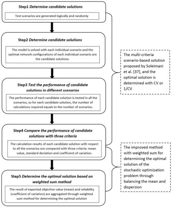
optimization problem and a clearer managerial meaning. Figure2presents the solutions procedures of the method, the difference between the improved solution method, and the original solution method is also presented in the figure.
=
Figure 2.Procedures of the improved multi-criteria scenario-based solution method.
Mean value is a very important criterion to evaluate the performance of a series of data (in this case, the optimal costs of reverse logistics network of WEEE with respect to the test scenarios); however, more comprehensive evaluation criteria are needed for reliable and robust decision-making in an uncertain environment. In the multi-criteria scenario-based method, it is important to consider how closely the data approach the mean value, and this requires knowledge about the dispersion of data evaluated by standard deviation. Standard deviation is a well-developed and extensively applied tool used for data analysis in many fields—for example, in the manufacturing industry, the quality of a batch of products can be evaluated by standard deviation; a smaller standard deviation shows a better distribution of the product samples around the required quality level. In the solution method developed by Soleimani et al. [37], the reciprocal of coefficient of variation is applied to connect the mean value and the standard deviation and to determine the optimal solution of the stochastic programming. The basic idea for this solution method is to simultaneously maximize the profit of the supply chain (mean value) and the reliability and robustness of data dispersion or the risk (standard deviation); however, this method has two drawbacks from both mathematical and managerial perspectives.
(1) From a mathematical perspective, Soleimani et al.’s method is only capable of solving the max-minandmin-maxproblems [37]. For example, it is able to resolve the problem considering the maximum profit and the minimum risk or maximum reliability of the supply chain. However, for the problem formulated in this paper, which is amin-minproblem aiming at determining the minimum costs and minimum data dispersion, this solution method is ineffective.
(2) From a managerial perspective, the managerial meaning of coefficient of variation and its reciprocal are associated with the relative data dispersion compared with the absolute data dispersion determined by standard deviation, but it is not a dedicated tool for determining the optimal solution of a stochastic optimization problem. The theoretical justification of Soleimani et al.’s method [37] is not strong enough to enable comprehensive managerial interpretation. Furthermore, the data dispersion evaluated by standard deviation is significantly affected by the mean value, and this may lead to misinterpretation of the real shape of data dispersion.
In order to solve the aforementioned problems, we improve the multi-criteria scenario-based solution method. First, in our method, coefficient of variation is used to evaluate the reliability and robustness of data dispersion instead of standard deviation, and the managerial meaning of coefficient of variation is introduced. After that, a normalized weighted sum method is applied to aggregate the mean value and coefficient of variation, and the performance of the candidate solutions is evaluated by both expected objective value (mean value) and reliability (coefficient of variation) in order to find the most economic efficient, reliable, and robust solution to the stochastic optimization problem.
Standard deviation is an absolute measurement of data dispersion and is heavily affected by the mean value; if the mean value is different, comparison of standard deviation may not be an appropriate way of evaluating the data dispersion, so another indicator, coefficient of variation, is used to evaluate the reliability of the results. Coefficient of variation, alternatively known as coefficient of dispersion, incorporates both the standard deviation and the mean, and is a unitless indicator applied for measuring the relative dispersion of a series of data [47]:
Coe f f icient o f variation= Standard deviation
Mean . (30)
component B (0.15) is three times that of component A (0.05), which means the quality of test samples of component A is much better due to the more centered data distribution relative to its mean value. The optimal solution of the stochastic optimization problem is the one with the lowest expected objective costs (mean value) and the most reliable performance (coefficient of variation), but the best performance of those two objectives is usually not obtained in the same candidate solution. It is important to incorporate both criteria in the design of a reverse logistics system for WEEE. In this paper, we use the weighted sum method to combine the two criteria for selecting the optimal solution of the stochastic optimization problem, and this enables interactions between the subjective input from decision-makers (weight of each criterion) and the objective values of system performance. Furthermore, it is noted that, because of the different measures of units, the two evaluation criteria, mean value and coefficient of variation, are first normalized, as shown in Equation (31):
minOverall Per f omancecand.=WM
Meancand.
Meanmin
+WCCoe f f icient o f variationcand. Coe f f icient o f variationmin
. (31)
In Equation (31),MeanminandCoe f f icient o f variationminare minimum achievable values of the mean and coefficient of variation, andMeancand.andCoe f f icient o f variationcand.are the mean and coefficient of variation of each candidate solution. Through the improvement of the multi-criteria scenario-based solution method, the two drawbacks of the original method can be properly resolved. First, the evaluation of data dispersion by coefficient of variation is a better indicator for the reliability and robustness of reverse logistics system design of WEEE compared with standard deviation. Second, from a mathematical perspective, the introduction of normalized weighted sum method enables the multi-criteria scenario-based solution method to resolve not onlymax-minandmin-maxbut also min-minandmax-maxstochastic optimization problems. Third, the improved solution method provides a more reasonable aggregation of the expected optimal value and the reliability, which enables better interpretation of the result.
4. Numerical Experiment
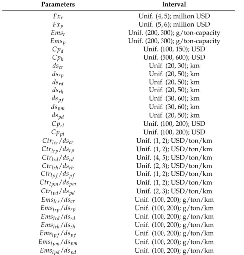
In order to illustrate the applicability of the proposed stochastic optimization programming and the improved solution method in the design and planning of a reverse logistics system for WEEE, a numerical experiment is performed in this section. The numerical experiment includes 10 local collection sites, 5 potential locations for regional collection centers, 5 potential locations for recycling plants, 1 hazardous waste management system, 2 disposal sites, 3 product markets, and 3 material markets. The relevant parameters used in the numerical experiment are randomly generated in a uniformly distributed interval, as shown in Table1.
Table 1.Parameter generation in the numerical experiment.
Parameters Interval
Fxr Unif. (4, 5); million USD
Fxp Unif. (5, 6); million USD
Emsr Unif. (200, 300); g/ton-capacity
Emsp Unif. (200, 300); g/ton-capacity
Cpd Unif. (100, 150); USD
Cph Unif. (500, 600); USD
dscr Unif. (20, 30); km
dsrp Unif. (20, 50); km
dsrd Unif. (20, 50); km
dsrh Unif. (20, 50); km
dsp f Unif. (30, 60); km
dspm Unif. (30, 60); km
dspd Unif. (20, 50); km
Cprl Unif. (100, 200); USD
Cppl Unif. (100, 200); USD
Ctrlcr/dscr Unif. (1, 2); USD/ton/km
Ctrlrp/dsrp Unif. (1, 2); USD/ton/km
Ctrlrd/dsrd Unif. (4, 5); USD/ton/km
Ctrlrh/dsrh Unif. (2, 3); USD/ton/km
Ctrl p f/dsp f Unif. (1, 2); USD/ton/km
Ctrl pm/dspm Unif. (1, 2); USD/ton/km
Ctrl pd/dspd Unif. (2, 3); USD/ton/km
Emslcr/dscr Unif. (100, 200); g/ton/km
Emslrp/dsrp Unif. (100, 200); g/ton/km
Emslrd/dsrd Unif. (100, 200); g/ton/km
Emslrh/dsrh Unif. (100, 200); g/ton/km
Emsl p f/dsp f Unif. (100, 200); g/ton/km
Emsl pm/dspm Unif. (100, 200); g/ton/km
Emsl pd/dspd Unif. (100, 200); g/ton/km
Table 2.Parameter generation with respect to different types of WEEE.
Parameters Interval
Type A Type B Type C
Cols
lc Unif. (500, 600); ton Unif. (1000, 2000); ton Unif. (1000, 2000); ton
PCpsf l Unif. (200, 300); USD/ton Unif. (150, 250); USD/ton Unif. (150, 250); USD/ton
PCms
ml Unif. (100, 150); USD/ton Unif. (100, 200); USD/ton Unif. (100, 200); USD/ton
Capacityrl 4000; ton 8000; ton 10,000; ton
Capacitypl 3000; ton 5000; ton 8000; ton
ϕl p 50% 60% 60%
ϕld 20% 20% 30%
ϕlh 30% 20% 10%
ϑl f 30% 30% 40%
ϑlm 30% 40% 50%
ϑld 40% 30% 10%
for the price of recycled products, and two scenarios for the price of recycled materials based upon the uniformly distributed intervals. In total, eight test scenarios (s1,s2,s3,s4,s5,s6,s7, ands8) are generated through the combination of the possibilities of different uncertain parameters.
In addition to the basic and test scenarios, we also generated two benchmarking scenarios: the best-case scenario and the worst-case scenario. In the best-case scenario, the amount of WEEE collected at local collection sites reaches its lower limit while the prices for both recycled products and materials achieve their upper limits (Cols9
ac = 500 tons, Colbcs9 = 1000 tons, Colccs9= 1000 tons, PCpsf a9 = 300 USD/ton, PCpsf b9 = 250 USD/ton, PCpsf c9 = 250 USD/ton, PCmsma9 = 150 USD/ton, PCmsmb9 = 200 USD/ton and PCmsmc9 = 200 USD/ton); this means the reverse logistics system deals with the minimum amount of WEEE with the highest selling price from the recycled products and materials. In the worst-case scenario, the setting of uncertain parameters is an opposite manner (Colsac10= 600 tons,Colbcs10= 2000 tons, Colccs10 = 2000 tons,PCpsf a10 = 200 USD/ton, PCpsf b10= 150 USD/ton,PCpsf c10= 150 USD/ton,PCmsma10= 100 USD/ton,PCmsmb10= 100 USD/ton and PCms10
mc = 100 USD/ton).
The stochastic programming model is coded in Lingo 11.0 optimization package and the computation of all scenarios is performed on a personal laptop with Intel Core2 duo 2.52 GHz CPU and 4 GB RAM with Windows 7 operating system. At first, the optimal solutions of each individual scenario are calculated as the candidate solutions of the stochastic optimization problem. The problem of each scenario includes 632 decision variables, of which 10 are integers, and all the scenarios can be resolved within 30 s.
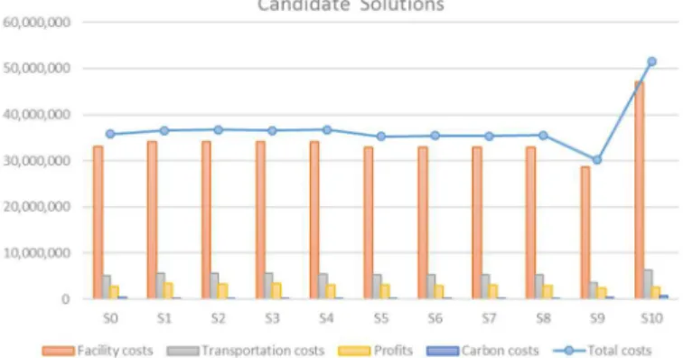
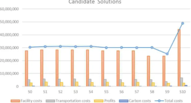
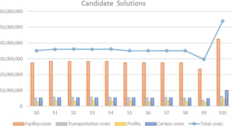
Figure3shows the optimal solutions of each individual scenario. As illustrated in the figure, the range of the solution area is 21,411,780 USD (71%), defined by the best-case scenarios9and the worst case scenarios10. However, when the extreme conditionss9ands10are not taken into account, the range of the optimal solutions of the test scenarios (s0–s8) is significantly reduced to 1,429,750 USD (4%). In this case, the mean value is 35,996,637 USD, which leads to a relatively fair distribution of the optimal solutions:s1,s2,s3, ands4have better performance, whiles0,s5,s6,s7, ands8are slightly below the mean value.
Figure 3.Candidate solutions of the stochastic optimization problem.
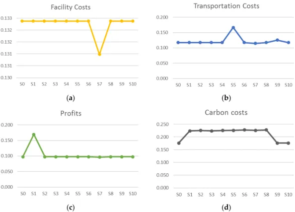
respectively. However, the contribution of carbon costs is relatively insignificant compared with other types of costs in this example.
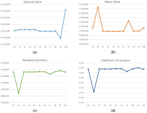
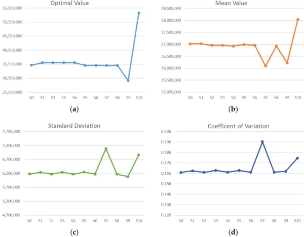
The candidate solutions represent the best performance that can be achieved in each individual scenario, but our objective is to find the optimal and most reliable and robust solution through all the possible scenarios. Therefore, the performance of each candidate solution is tested through all the test scenarios; in this example, each candidate solution is calculated 11 times for scenarioss0–s10, so in total 121 calculations are performed in this step. The result is presented in AppendixA(TableA1), and Figure4illustrates the comparison of the performance of each candidate solution through four criteria: optimal costs, mean costs, standard deviation, and coefficient of variation. Based on the computational results of the example, some managerial implications are discussed as follows.
(1) As shown in Figure4a, the best solution of individual optimal costs is achieved in scenarios5 with the lowest system costs of 35,306,520 USD. The optimal cost of the deterministic scenarios0 is the median of the problem, and the optimal costs of scenarioss1,s2,s3,s4, ands10are higher than the median value, while scenarioss5,s6,s7,s8, ands9have a better performance in their individual optimal costs.
(2) As shown in Figure4b, when the candidate solutions are evaluated through all the test scenarios, the best solution of the mean costs is 36,997,582 USD, achieved in scenarios4, and the worst solution is found for scenario s1, with 37,107,575 USD. It is noteworthy that, in terms of the mean costs, the performance of scenarioss2,s3,s4,s6,s8, ands9is close to the best performance. Furthermore, it is also observed that the change of mean costs is not correlated to the change of optimal individual costs, which means the better optimal individual costs may not lead to a better overall economic performance in most cases.
(3) As shown in Figure4c, when the candidate solutions are evaluated by standard deviation, the best solution is obtained via scenarios1, with the lowest standard deviation at 4,837,063.5 USD, which is far better than the other candidate solutions. This illustrates that the result of candidate solution s1tested with all possible scenarios has a more centered distribution around the mean value. (4) As shown in Figure4d, in terms of the performance of the coefficient of variation, the best solution
is obtained in scenarios2, with the lowest value of coefficient of variation at 0.1303524, which is far better than the other candidate solutions. The second best solution in terms of the coefficient of variation is achieved in scenarios7.
(5) Comparing Figure 4c with Figure 4d, it is observed that the change of the performance of candidate solutions with respect to standard deviation and coefficient of variation is quite similar, and the influence of the mean costs seems insignificant in this example. This result can be explained by the significant difference in the ranges of mean values and standard deviation. The range of the mean value is only 0.3%, which means the difference between the best and the worst solution is not significant. However, the range between the best solution and the worst solution in standard deviation is 7.2%, which is 24 times higher than that of the mean value, so standard deviation has a much more significant influence on coefficient of variation in this example. (6) In this example, Meanmin is 36,997,582 USD, obtained from candidate solution s4, and
(a) (b)
(c) (d)
Figure 4. Comparison of the evaluation criteria in candidate solutions: (a) Optimal costs; (b) mean Figure 4. Comparison of the evaluation criteria in candidate solutions: (a) Optimal costs; (b) mean costs; (c) standard deviation; (d) coefficient of variation.
(a) (b)
(c) (d)
Figure 5. Comparison of the reliability of different cost components in candidate solutions: (a) Figure 5. Comparison of the reliability of different cost components in candidate solutions: (a) Coefficient of variation of the facility costs; (b) coefficient of variation of the transportation costs; (c) coefficient of variation of the profits; (d) coefficient of variation of the carbon cost.
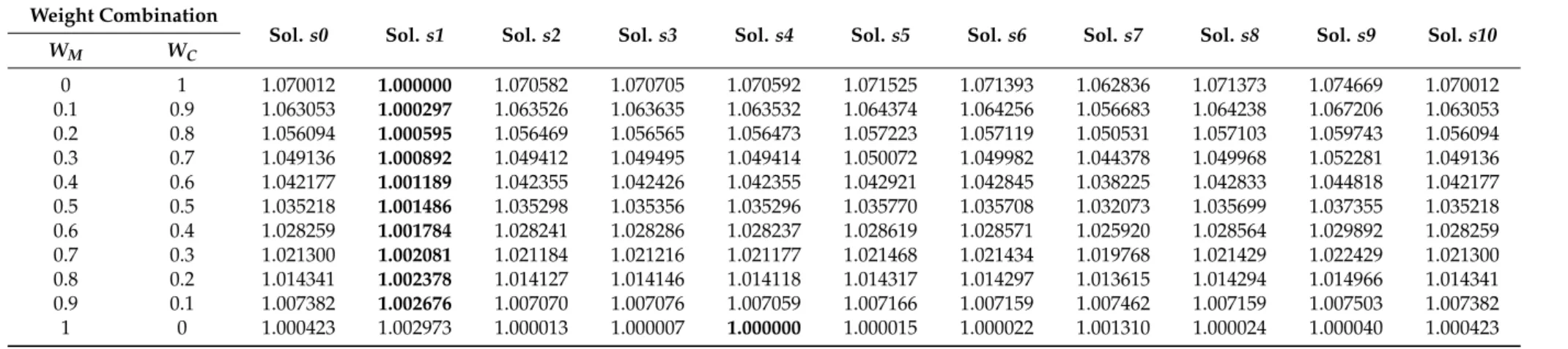
Table 3.Sensitivity analysis of the result with respect to the change of weight combination.
Weight Combination
Sol.s0 Sol.s1 Sol.s2 Sol.s3 Sol.s4 Sol.s5 Sol.s6 Sol.s7 Sol.s8 Sol.s9 Sol.s10
WM WC
5. Sensitivity Analysis
We are interested in the influence of the change of some key parameters in the design of reverse logistics system for WEEE, and two sensitivity analyses (SAandS-B) are performed in this section. The facility capacity limitation is the bottleneck of the reverse logistics system for WEEE in the previous section. The literature has shown that facility expansion at the same location is much more efficient in dealing with increased customer demand than opening new facilities [50]. Therefore, in the first sensitivity analysisS-A, we increase the facility capacity of different types of WEEE by 100% at regional collection centers and recycling plants, and the fixed facility costs are increased by 40% due to the increase in the resources invested in facility expansion, i.e., equipment, personnel, etc.
The result of sensitivity analysisS-Ais illustrated in AppendixB(TableB1), Figures6and7, and Table4. As illustrated in the figures and tables, the overall system costs are reduced by approximately 15% compared with the result of the previous numerical experiment, the optimal mean value is achieved at candidate solutions0, and the optimal coefficient of variation is obtained at candidate solutions9. When the weights of expected objective value and reliability are identical, the optimal solution is 1.002680, obtained at candidate solutions9, potential locationr1is selected to open the regional collection center, and potential locationp5 is selected for the new recycling plant. It is noteworthy that, with the increase in facility capacity, only two new facilities are opened in sensitivity analysisS-Afor the treatment of WEEE, and the overall facility costs are significantly reduced due to the decreased number of facilities opened, even though the fixed operating costs of each individual facility increase by 40%. This result has revealed the effectiveness of capacity expansion at existing facilities. Compared with opening new facilities, the possible capacity expansion may drastically reduce the overall system costs due to the cost savings from construction, aggregation of transportation, and economy of scale. This result is valuable for decision-making about reverse logistics system design and planning for treating the increased amount of WEEE, particularly from a long-term perspective.
Compared with other types of costs, the carbon emissions costs are relatively insignificant in the overall system costs of the reverse logistics system for WEEE. We are interested in finding out whether a more stringent environmental policy can play an important role in the design of a reverse logistics system for WEEE. In the second sensitivity analysisS-B, two changes are made to minimize the environmental impacts of the reverse logistics system for WEEE. First, the carbon cap is reduced to 0, which means all the carbon emissions from the reverse logistics system will be charged. In addition, the unit cost for buying carbon credits is increased 10 times, which means much more will be paid for the carbon emissions. Sensitivity analysisS-Bis conducted to test the result of the problem in an extreme condition in which environmental sustainability is made one of the first priorities, and it can be used for policy-making and a reconfiguration of the reverse logistics system in the coming years.
(a) (b)
(c) (d)
Figure 7. Comparison of the evaluation criteria in candidate solutions of sensitivity analysis S-A: (a)
Figure 7.Comparison of the evaluation criteria in candidate solutions of sensitivity analysisS-A: (a) Optimal costs; (b) mean costs; (c) standard deviation; (d) coefficient of variation.
The result of the sensitivity analysisS-Bis illustrated in AppendixB(TableB2), Figures8and9, and Table5. As shown in the figures and tables, the stringent environmental requirements lead to much higher overall costs for the reverse logistics system for WEEE due to the great increase in carbon emissions costs. The optimal mean value and coefficient of variation are obtained at candidate solutions s0ands9, respectively. When WMequals 0.5 andWC equals 0.5, the optimal solution is 1.004995, achieved at candidate solutions9, and potential locationsr1andp5are selected for new facilities. The facility selection is the same as that in sensitivity analysisS-A, which shows the consistency between economic efficiency and environmental impact. In other words, an optimal and reliable configuration of a reverse logistics system for WEEE through location optimization and transportation aggregation may bring both economic and environmental benefits.
(a) (b)
(c) (d)
Figure 9. Comparison of the evaluation criteria in candidate solutions of sensitivity analysis S-B: (a)
Figure 9.Comparison of the evaluation criteria in candidate solutions of sensitivity analysisS-B: (a) Optimal costs; (b) mean costs; (c) standard deviation; (d) coefficient of variation.
Table 4.Sensitivity analysis of the results with respect to the change of weight combination (S-A).
Weight Combination
Sol.s0 Sol.s1 Sol.s2 Sol.s3 Sol.s4 Sol.s5 Sol.s6 Sol.s7 Sol.s8 Sol.s9 Sol.s10
WM WC
0 1 1.000000 1.012538 1.001633 1.015303 1.002341 1.015362 1.002212 1.015867 1.002596 1.005359 1.103707 0.1 0.9 1.002578 1.013821 1.003791 1.016100 1.004321 1.016259 1.004313 1.016609 1.004564 1.004823 1.099090 0.2 0.8 1.005155 1.015104 1.005949 1.016897 1.006301 1.017156 1.006415 1.017351 1.006532 1.004287 1.094472 0.3 0.7 1.007733 1.016387 1.008107 1.017694 1.008281 1.018054 1.008516 1.018092 1.008500 1.003752 1.089854 0.4 0.6 1.010310 1.017670 1.010266 1.018491 1.010262 1.018951 1.010617 1.018834 1.010468 1.003216 1.085237 0.5 0.5 1.012888 1.018952 1.012424 1.019288 1.012242 1.019849 1.012718 1.019576 1.012435 1.002680 1.080619 0.6 0.4 1.015465 1.020235 1.014582 1.020085 1.014222 1.020746 1.014819 1.020317 1.014403 1.002144 1.076002 0.7 0.3 1.018043 1.021518 1.016740 1.020882 1.016202 1.021644 1.016921 1.021059 1.016371 1.001608 1.071384 0.8 0.2 1.020620 1.022801 1.018898 1.021679 1.018183 1.022541 1.019022 1.021800 1.018339 1.001072 1.066766 0.9 0.1 1.023198 1.024084 1.021057 1.022476 1.020163 1.023438 1.021123 1.022542 1.020307 1.000536 1.062149 1 0 1.025775 1.025367 1.023215 1.023273 1.022143 1.024336 1.023224 1.023284 1.022275 1.000000 1.057531
Table 5.Sensitivity analysis of the result with respect to the change of weight combination (S-B).
Weight Combination
Sol.s0 Sol.s1 Sol.s2 Sol.s3 Sol.s4 Sol.s5 Sol.s6 Sol.s7 Sol.s8 Sol.s9 Sol.s10
WM WC
6. Conclusions
Today, the increased public concern about sustainable development and more stringent environmental regulations have become important driving forces for value recovery from end-of-life and end-of use products through reverse logistics. This paper presents a novel stochastic mixed integer programming model for the design of a generic multi-source, multi-echelon, and capacitated reverse logistics system for WEEE in an economic efficient and environmental friendly manner. The model aims at minimizing the overall costs of the reverse logistics system for WEEE through location optimization and transportation planning, and the amount of WEEE generated at local collection sites, price of recycled products, and recycled materials are considered as uncertain parameters. Furthermore, the model takes into account the environmental impacts of reverse logistics; in this paper, the environmental impacts are evaluated in terms of carbon emissions costs. The proposed stochastic optimization model is resolved with an improved multi-criteria scenario-based solution method and coded in Lingo 11.0 optimization solver, and a numerical example and sensitivity analyses are conducted in order to illustrate the application of the model and provide managerial insights for decision-making. The main contributions of the paper are summarized as follows:
(1) The paper provides a novel stochastic optimization model for the design of a generic reverse logistics system for WEEE. Reverse logistics is characterized as having a high level of uncertainty, so the modelling and formulation of some uncertain parameters are of significant importance. (2) Compared with previous mathematical models, the model proposed in this paper considers the
environmental impacts of the reverse logistics system for WEEE, and the minimization of carbon emissions is also a very important consideration of the model.
(3) The model is resolved with the multi-criteria scenario-based solution method in order to find the most economically efficient and reliable solution to the stochastic optimization problem. The expected objective value and reliability are evaluated by the mean and coefficient of variation, and normalized weighted sum formulation is applied to combine the two evaluation criteria. The solution method enables interactions between the subjective evaluation from the decision makers and the objective system values, so the result achieved is more reliable and robust. In addition, our improved solution method also resolves the deficiencies of the original solution method, and is capable of solvingmin-minandmax-maxoptimization problems. In addition, the managerial meaning of the solution method is explicitly explained in this paper.
(4) The numerical experiment and sensitivity analyses provide valuable managerial insights into the design of a reverse logistics system for WEEE. For example, capacity expansion at existing facilities may be a more economically efficient way for dealing with an increased amount of WEEE, and both economic and environmental performance may be improved simultaneously with location optimization and transportation aggregation. In addition, the managerial insight from the system design and planning of a reverse logistics network of WEEE may also provide valuable information for the government in determining a subsidy scheme for companies performing WEEE treatment.
a real-world case study of the design and planning of the reverse logistics system for WEEE will be expected in the future.
Acknowledgments:The authors would like to express their gratitude to the editors and reviewers who provide valuable comments and suggestions for improving the quality and presentation of the paper. The research result presented in this paper is the further development of an earlier paper, “A reverse logistics network design model for sustainable treatment of multi-sourced waste of electrical and electronic equipment (WEEE)”, presented at the 4th IEEE International Conference on Cognitive Infocommunications. The current research was conducted with the support from the TARGET Project financed by the Northern Periphery and Arctic Programme (NPA). The article processing charge was financially supported by the Open Access Fund at UiT—The Arctic University of Norway.
Author Contributions: Hao Yu formulated the stochastic optimization model, designed the solution method, conducted the numerical experiment, and wrote the first draft of the paper. Wei Deng Solvang thoroughly reviewed and improved the paper.
Appendix A. Computational Results of Numerical Example
Table A1.Scenario-based overall system costs of the reverse logistics system for WEEE.
Sol.s0 Sol.s1 Sol.s2 Sol.s3 Sol.s4 Sol.s5 Sol.s6 Sol.s7 Sol.s8 Sol.s9 Sol.s10
s0 35,801,630 35,952,130 35,801,630 35,801,630 35,801,630 35,801,630 35,801,630 35,875,160 35,801,630 35,801,630 35,801,630
s1 36,718,370 36,548,660 36,718,370 36,718,370 36,718,370 36,718,370 36,718,370 36,746,110 36,718,370 36,718,370 36,718,370
s2 36,893,640 37,110,980 36,726,620 36,893,640 36,893,640 36,893,640 36,893,640 36,921,500 36,893,640 36,893,640 36,893,640
s3 36,727,900 36,783,460 36,727,900 36,558,310 36,727,900 36,727,900 36,727,900 36,755,780 36,727,900 36,727,900 36,727,900
s4 36,908,510 37,181,410 36,908,510 36,908,510 36,736,270 36,908,510 36,908,510 36,936,390 36,908,510 36,908,510 36,908,510
s5 35,472,470 35,472,470 35,472,470 35,472,470 35,472,470 35,306,520 35,472,470 35,472,470 35,472,470 35,472,470 35,472,470
s6 35,633,550 35,825,670 35,633,550 35,633,550 35,633,550 35,633,550 35,470,410 35,633,550 35,633,550 35,633,550 35,633,550
s7 35,494,550 35,519,400 35,494,550 35,494,550 35,494,550 35,494,550 35,494,550 35,328,710 35,494,550 35,494,550 35,494,550
s8 35,655,000 35,871,970 35,655,000 35,655,000 35,655,000 35,655,000 35,655,000 35,655,640 35,492,600 35,655,000 35,655,000
s9 30,292,120 31,104,970 30,292,120 30,292,120 30,292,120 30,292,120 30,292,120 30,607,740 30,292,120 30,136,120 30,292,120
s10 51,547,900 50,812,200 51,547,900 51,547,900 51,547,900 51,547,900 51,547,900 51,573,440 51,547,900 51,547,900 51,547,900 MV1 37,013,240 37,107,575 36,998,056 36,997,823 36,997,582 36,998,154 36,998,409 37,046,045 36,998,476 36,999,058 37,013,240 SD2 5,162,559.3 4,837,063.5 5,163,191.8 5,163,749.7 5,163,169.9 5,167,752 5,167,151.5 5,132,479.4 5,167,062.2 5,183,042.5 5,162,559.3 CV3 0.1394787 0.1303524 0.139553 0.139569 0.1395542 0.1396759 0.1396587 0.1385432 0.139656 0.1400858 0.1394787
Appendix B. Computational Result of Sensitivity Analysis
Table B1.Scenario-based overall system costs of the reverse logistics system for WEEE in sensitivity analysis (A).
Sol.s0 Sol.s1 Sol.s2 Sol.s3 Sol.s4 Sol.s5 Sol.s6 Sol.s7 Sol.s8 Sol.s9 Sol.s10
s0 30,433,820 30,710,800 30,451,520 30,593,350 30,334,070 30,710,800 30,451,520 30,593,350 30,334,070 29,651,950 31,215,700
s1 31,251,300 30,937,490 31,134,170 30,789,760 31,176,440 30,747,490 31,134,170 30,789,760 31,176,440 30,416,190 32,086,410
s2 31,408,420 31,530,740 31,091,320 31,573,010 31,294,760 31,530,740 31,252,500 31,573,010 31,294,760 30,573,310 32,243,530
s3 31,586,510 31,183,690 31,570,370 30,959,830 31,511,650 31,183,690 31,570,370 31,124,970 31,511,650 30,751,400 32,421,620
s4 31,394,940 31,618,250 31,340,010 31,559,530 31,113,650 31,618,250 31,340,010 31,559,530 31,281,290 30,559,830 32,230,050
s5 30,670,490 30,210,790 30,537,930 30,247,360 30,574,500 30,049,090 30,537,930 30,247,360 30,574,500 29,898,040 31,442,940
s6 30,478,020 30,585,080 30,329,100 30,621,640 30,365,660 30,585,080 30,171,130 30,621,640 30,365,660 29,705,560 31,250,470
s7 30,649,910 30,293,480 30,620,610 30,226,780 30,553,910 30,293,480 30,620,610 30,065,270 30,553,910 29,877,450 31,422,360
s8 30,416,720 30,644,330 30,376,820 30,577,630 30,310,120 30,644,330 30,376,820 30,577,630 30,187,320 29,626,270 31,207,180
s9 25,749,000 25,939,050 25,768,800 25,849,950 25,679,700 25,939,050 25,768,800 25,849,950 25,679,700 25,212,750 26,285,250
s10 45,929,180 46,175,180 45,874,080 46,115,780 45,814,680 46,175,180 45,874,080 46,115,780 45,814,680 44,901,680 48,997,110
MV1 31,815,301 31,802,625 31,735,885 31,737,693 31,702,649 31,770,653 31,736,176 31,738,023 31,706,725 31,015,857 32,800,238
SD2 4,950,109.6 5,010,178.7 4,945,815.7 5,013,603.6 4,944,127.9 5,019,098.1 4,948,722.4 5,016,440 4,946,024 4,851,587.7 5,632,609.1
CV3 0.155589 0.1575398 0.155843 0.15797 0.1559531 0.1579791 0.1559332 0.1580577 0.1559928 0.1564228 0.1717246
1MV: Mean value.2SD: Standard deviation.3CV: Coefficient of variance (CV = SD/MV).
Table B2.Scenario-based overall system costs of the reverse logistics system for WEEE in sensitivity analysis (B).
Sol.s0 Sol.s1 Sol.s2 Sol.s3 Sol.s4 Sol.s5 Sol.s6 Sol.s7 Sol.s8 Sol.s9 Sol.s10
s0 35,217,930 35,511,820 35,252,540 35,394,370 35,135,090 35,511,820 35,252,540 35,394,370 35,135,090 34,452,970 36,016,720
s1 36,188,520 36,055,660 36,071,390 35,726,980 36,113,660 35,684,710 36,071,390 35,726,980 36,113,660 35,353,410 37,023,630
s2 36,284,990 36,407,310 36,111,890 36,449,570 36,171,330 36,407,310 36,129,070 36,449,570 36,171,330 35,449,880 37,387,200
s3 36,552,090 36,149,270 36,535,950 36,073,380 36,477,230 36,149,270 36,535,950 36,090,550 36,477,230 35,716,980 37,387,200
s4 36,267,670 36,490,970 36,212,730 36,432,250 36,129,610 36,490,970 36,212,730 36,432,250 36,154,010 35,432,560 37,102,780
s5 35,558,890 35,099,190 35,426,330 35,135,750 35,462,890 35,081,860 35,426,330 35,135,750 35,462,890 34,786,430 36,331,340
s6 35,282,160 35,389,220 35,133,240 35,425,790 35,169,800 35,389,220 35,115,900 35,425,790 35,169,800 34,509,710 36,054,620
s7 35,533,790 35,177,360 35,504,490 35,110,650 35,437,790 35,177,360 35,504,490 35,093,320 35,437,790 34,761,330 36,306,240
s8 35,219,260 35,446,870 35,179,360 35,380,170 35,112,660 35,446,870 35,179,360 30,325,590 35,127,370 34,428,810 36,009,720
s9 30,224,640 30,414,690 30,244,440 30,325,590 30,155,340 30,414,690 30,244,440 25,849,950 30,155,340 29,673,020 30,760,890
s10 54,892,650 55,138,650 54,837,550 55,079,250 54,778,150 55,138,650 54,837,550 55,079,250 54,778,150 53,865,150 57,978,850
MV1 37,020,235 37,025,546 36,955,446 36,957,614 36,922,141 36,990,248 36,955,432 36,091,215 36,925,696 36,220,932 38,032,654
SD2 6,176,398.2 6,235,000.1 6,171,274.3 6,238,725 6,168,802.5 6,242,297.6 6,171,556.3 7,084,390.6 6,168,063 6,081,694.7 6,865,778.5
CV3 0.1668384 0.1683972 0.1669923 0.1688076 0.167076 0.1687552 0.1669999 0.1962913 0.1670399 0.1679055 0.1805232
References
1. Goosey, M. End-of-life electronics legislation-an industry perspective. Circuit World 2004, 30, 41–45. [CrossRef]
2. Yu, H.; Solvang, W.D. A reverse logistics network design model for sustainable treatment of multi-sourced waste of electrical and electronic equipment (WEEE). In Proceedings of the 4th IEEE International Conference on Cognitive Infocommunications (CogInfoCom), Budapest, Hungary, 2–5 December 2013; pp. 595–600. 3. Wagner, T.P. Shared responsibility for managing electronic waste: A case study of maine, USA.Waste Manag.
2009,29, 3014–3021. [CrossRef] [PubMed]
4. Achillas, C.; Vlachokostas, C.; Aidonis, D.; Moussiopoulos, N.; Iakovou, E.; Banias, G. Optimising reverse logistics network to support policy-making in the case of electrical and electronic equipment.Waste Manag.
2010,30, 2592–2600. [CrossRef] [PubMed]
5. Bigum, M.; Brogaard, L.; Christensen, T.H. Metal recovery from high-grade WEEE: A life cycle assessment.
J. Hazard. Mater.2012,207, 8–14. [CrossRef] [PubMed]
6. Rahmani, M.; Nabizadeh, R.; Yaghmaeian, K.; Mahvi, A.H.; Yunesian, M. Estimation of waste from computers and mobile phones in Iran.Resour. Conserv. Recycl.2014,87, 21–29. [CrossRef]
7. Jaiswal, A.; Samuel, C.; Patel, B.S.; Kumar, M. Go green with WEEE: Eco-friendly approach for handling e-waste.Procedia Comput. Sci.2015,46, 1317–1324. [CrossRef]
8. Cao, J.; Chen, Y.; Shi, B.; Lu, B.; Zhang, X.; Ye, X.; Zhai, G.; Zhu, C.; Zhou, G. WEEE recycling in zhejiang province, china: Generation, treatment, and public awareness.J. Clean. Prod.2016,127, 311–324. [CrossRef] 9. Courtering WEEE Illegal Trade (CWIT) Summary Report. Available online:
http://www.cwitproject.eu/wp-content/uploads/2015/09/CWIT-Final-Report.pdf (accessed on 9 December 2016).
10. Salhofer, S.; Steuer, B.; Ramusch, R.; Beigl, P. WEEE management in Europe and China—A comparison.
Waste Manag.2016,57, 27–35. [CrossRef] [PubMed]
11. Orlins, S.; Guan, D. China’s toxic informal e-waste recycling: Local approaches to a global environmental problem.J. Clean. Prod.2016,114, 71–80. [CrossRef]
12. Yu, H.; Solvang, W.D. A general reverse logistics network design model for product reuse and recycling with environmental considerations.Int. J. Adv. Manuf. Technol.2016,87, 2693–3711. [CrossRef]
13. Rogers, D.S.; Tibben-Lembke, R. An examination of reverse logistics practices. J. Bus. Logist. 2001, 22, 129–148. [CrossRef]
14. Fleischmann, M.; Bloemhof-Ruwaard, J.M.; Dekker, R.; Van der Laan, E.; Van Nunen, J.A.; Van Wassenhove, L.N. Quantitative models for reverse logistics: A review.Eur. J. Oper. Res.1997,103, 1–17. [CrossRef]
15. Carter, C.R.; Ellram, L.M. Reverse logistics: A review of the literature and framework for future investigation.
J. Bus. Logist.1998,19, 85–102.
16. Pokharel, S.; Mutha, A. Perspectives in reverse logistics: A review.Resour. Conserv. Recycl.2009,53, 175–182. [CrossRef]
17. Govindan, K.; Soleimani, H.; Kannan, D. Reverse logistics and closed-loop supply chain: A comprehensive review to explore the future.Eur. J. Oper. Res.2015,240, 603–626. [CrossRef]
18. He, W.; Li, G.; Ma, X.; Wang, H.; Huang, J.; Xu, M.; Huang, C. WEEE recovery strategies and the WEEE treatment status in china.J. Hazard. Mater.2006,136, 502–512. [CrossRef] [PubMed]
19. Oguchi, M.; Sakanakura, H.; Terazono, A. Toxic metals in WEEE: Characterization and substance flow analysis in waste treatment processes.Sci. Total Environ.2013,463, 1124–1132. [CrossRef] [PubMed] 20. Xavier, L.H.; Adenso-Díaz, B. Decision models in e-waste management and policy: A review. InDecision
Models in Engineering and Management; Springer: Berlin, Germany, 2015; pp. 271–291.
21. Walther, G.; Spengler, T. Impact of WEEE-directive on reverse logistics in germany. Int. J. Phys. Distrib. Logist. Manag.2005,35, 337–361. [CrossRef]
22. Dat, L.Q.; Linh, D.T.T.; Chou, S.-Y.; Vincent, F.Y. Optimizing reverse logistic costs for recycling end-of-life electrical and electronic products.Expert Syst. Appl.2012,39, 6380–6387. [CrossRef]
23. Gomes, M.I.; Barbosa-Povoa, A.P.; Novais, A.Q. Modelling a recovery network for WEEE: A case study in portugal.Waste Manag.2011,31, 1645–1660. [CrossRef] [PubMed]
25. Quariguasi Frota Neto, J.; Walther, G.; Bloemhof, J.; Van Nunen, J.; Spengler, T. From closed-loop to sustainable supply chains: The WEEE case.Int. J. Prod. Res.2010,48, 4463–4481. [CrossRef]
26. Alumur, S.A.; Nickel, S.; Saldanha-da-Gama, F.; Verter, V. Multi-period reverse logistics network design.
Eur. J. Oper. Res.2012,220, 67–78. [CrossRef]
27. Grunow, M.; Gobbi, C. Designing the reverse network for WEEE in denmark.CIRP Ann. Manuf. Technol.
2009,58, 391–394. [CrossRef]
28. Capraz, O.; Polat, O.; Gungor, A. Planning of waste electrical and electronic equipment (WEEE) recycling facilities: Milp modelling and case study investigation.Flex. Serv. Manuf. J.2015,27, 479–508. [CrossRef] 29. Liu, H.; Lei, M.; Deng, H.; Leong, G.K.; Huang, T. A dual channel, quality-based price competition model for
the WEEE recycling market with government subsidy.Omega2016,59, 290–302. [CrossRef]
30. Manzini, R.; Bortolini, M. Strategic planning and operational planning in reverse logistics. A case study for italian WEEE. InEnvironmental Issues in Supply Chain Management; Springer: Berlin, Germany, 2012; pp. 107–130.
31. Yao, L.; He, W.; Li, G.; Huang, J. The integrated design and optimization of a WEEE collection network in shanghai, china.Waste Manag. Res.2013,31, 910–919. [CrossRef] [PubMed]
32. Tsai, W.H.; Hung, S.-J. Treatment and recycling system optimisation with activity-based costing in WEEE reverse logistics management: An environmental supply chain perspective. Int. J. Prod. Res. 2009, 47, 5391–5420. [CrossRef]
33. Mar-Ortiz, J.; Adenso-Díaz, B.; González-Velarde, J.L. Efficient vehicle routing practices for WEEE collection. InEnvironmental Issues in Supply Chain Management; Springer: Berlin, Germany, 2012; pp. 131–153.
34. Shokohyar, S.; Mansour, S. Simulation-based optimisation of a sustainable recovery network for waste from electrical and electronic equipment (WEEE).Int. J. Comput. Integr. Manuf.2013,26, 487–503. [CrossRef] 35. Ayvaz, B.; Bolat, B.; Aydın, N. Stochastic reverse logistics network design for waste of electrical and electronic
equipment.Resour. Conserv. Recycl.2015,104, 391–404. [CrossRef]
36. Fleischmann, M.; Krikke, H.R.; Dekker, R.; Flapper, S.D.P. A characterisation of logistics networks for product recovery.Omega2000,28, 653–666. [CrossRef]
37. Soleimani, H.; Seyyed-Esfahani, M.; Shirazi, M.A. A new multi-criteria scenario-based solution approach for stochastic forward/reverse supply chain network design.Ann. Oper. Res.2013. [CrossRef]
38. Govindan, K.; Rajendran, S.; Sarkis, J.; Murugesan, P. Multi criteria decision making approaches for green supplier evaluation and selection: A literature review.J. Clean. Prod.2015,98, 66–83. [CrossRef]
39. Diabat, A.; Abdallah, T.; Al-Refaie, A.; Svetinovic, D.; Govindan, K. Strategic closed-loop facility location problem with carbon market trading.IEEE Trans. Eng. Manag.2013,60, 398–408. [CrossRef]
40. Kannan, D.; Diabat, A.; Alrefaei, M.; Govindan, K.; Yong, G. A carbon footprint based reverse logistics network design model.Resour. Conserv. Recycl.2012,67, 75–79. [CrossRef]
41. Fahimnia, B.; Sarkis, J.; Dehghanian, F.; Banihashemi, N.; Rahman, S. The impact of carbon pricing on a closed-loop supply chain: An australian case study.J. Clean. Prod.2013,59, 210–225. [CrossRef]
42. Yu, H.; Solvang, W.D.; Yuan, S.; Yang, Y. A decision aided system for sustainable waste management.
Intell. Decis. Technol.2015,9, 29–40. [CrossRef]
43. Abdelaziz, F.B. Solution approaches for the multiobjective stochastic programming.Eur. J. Oper. Res.2012,
216, 1–16. [CrossRef]
44. Kaut, M.; Wallace, S.W. Evaluation of scenario-generation methods for stochastic programming.Pac. J. Optim.
2003,3, 257–271.
45. Niknam, T.; Azizipanah-Abarghooee, R.; Narimani, M.R. An efficient scenario-based stochastic programming framework for multi-objective optimal micro-grid operation.Appl. Energy2012,99, 455–470. [CrossRef] 46. Birge, J.R.; Louveaux, F.Introduction to Stochastic Programming; Springer Science & Business Media: New York,
NY, USA, 2011.
47. Brown, C.E. Coefficient of variation. InApplied Multivariate Statistics in Geohydrology and Related Sciences; Springer: Berlin, Germany, 1998; pp. 155–157.
48. Pishvaee, M.S.; Jolai, F.; Razmi, J. A stochastic optimization model for integrated forward/reverse logistics network design.J. Manuf. Syst.2009,28, 107–114. [CrossRef]
50. Melo, M.T.; Nickel, S.; Gama, F.S.D. Dynamic multi-commodity capacitated facility location: A mathematical modeling framework for strategic supply chain planning.Comput. Oper. Res.2006,33, 181–208. [CrossRef] 51. Crainic, T.G.; Hewitt, M.; Rei, W. Scenario grouping in a progressive hedging-based meta-heuristic for
stochastic network design.Comput. Oper. Res.2014,43, 90–99. [CrossRef]
52. Azadeh, A.; Sohrabi, P.; Saberi, M. A unique meta-heuristic algorithm for optimization of electricity consumption in energy-intensive industries with stochastic inputs. Int. J. Adv. Manuf. Technol. 2015,
78, 1691–1703. [CrossRef]
53. Mari, S.I.; Lee, Y.H.; Memon, M.S. Sustainable and Resilient Supply Chain Network Design under Disruption Risks.Sustainability2014,6, 6666–6686. [CrossRef]
54. Yu, H.; Solvang, W.D. An improved multi-objective programming with augmentedε-constraint method for hazardous waste location-routing problems.Int. J. Environ. Res. Public Health2016,13, 548. [CrossRef] [PubMed]
55. Yu, M.C.; Goh, M. A multi-objective approach to supply chain visibility and risk.Eur. J. Oper. Res.2014,233, 125–130. [CrossRef]
56. Sun, Y.; Lang, M.; Wang, D. Bi-objective modelling for hazardous materials road–rail multimodal routing problem with railway schedule-based space–time Constraints.Int. J. Environ. Res. Public Health2016,13, 762. [CrossRef] [PubMed]
57. Sun, Y.; Lang, M. Bi-objective optimization for multi-modal transportation routing planning problem based on Pareto optimality.J. Ind. Eng. Manag.2015,8, 1195–1217. [CrossRef]