PDF Fulltext | August 2016 Browse Articles 08 00754

(1)

Article

A Hybrid Multi-Step Rolling Forecasting Model

Based on SSA and Simulated Annealing—Adaptive

Particle Swarm Optimization for Wind Speed

Pei Du1_{, Yu Jin}1,_{* and Kequan Zhang}2

1 _{School of Statistics, Dongbei University of Finance and Economics, Dalian 116025, China;} [email protected]

2 _{Key Laboratory of Arid Climatic Change and Reducing Disaster of Gansu Province,}

College of Atmospheric Sciences, Lanzhou University, Lanzhou 730000, China; [email protected]

* Correspondence: [email protected]; Tel.: +86-411-8471-0451

Academic Editor: Andrew Kusiak

Received: 22 May 2016; Accepted: 27 July 2016; Published: 6 August 2016

Abstract:With the limitations of conventional energy becoming increasing distinct, wind energy is emerging as a promising renewable energy source that plays a critical role in the modern electric and economic fields. However, how to select optimization algorithms to forecast wind speed series and improve prediction performance is still a highly challenging problem. Traditional single algorithms are widely utilized to select and optimize parameters of neural network algorithms, but these algorithms usually ignore the significance of parameter optimization, precise searching, and the application of accurate data, which results in poor forecasting performance. With the aim of overcoming the weaknesses of individual algorithms, a novel hybrid algorithm was created, which can not only easily obtain the real and effective wind speed series by using singular spectrum analysis, but also possesses stronger adaptive search and optimization capabilities than the other algorithms: it is faster, has fewer parameters, and is less expensive. For the purpose of estimating the forecasting ability of the proposed combined model, 10-min wind speed series from three wind farms in Shandong Province, eastern China, are employed as a case study. The experimental results were considerably more accurately predicted by the presented algorithm than the comparison algorithms.

Keywords:renewable and sustainable energy; multi-step rolling wind speed forecasting; singular spectrum analysis; APSOSA algorithm

1. Introduction

Energy plays a vital part in modern social and economic development. Along with the rapid development of technology in the last few decades, energy demands continue to increase rapidly [1]. In accordance with the IEA World Energy Outlook 2010, China and India will be responsible for approximately 50% of the growth in global energy demand by 2050. The consumption of energy in China will be close to 70% greater than the energy consumed by the United States today. Second only to America, China will become the second leading energy-consuming country in the world. Nevertheless, China’s per capita energy consumption will remain lower than 50% of that of the USA [2]. Since conventional energy sources such as coal, natural gas, and oil for electricity generation are being quickly depleted, sufficient energy reserves and sustainable energy problems are garnering increased attention. Additionally, using traditional resources produces large amounts of carbon dioxide, which may lead to global warming, and is considered an international security threat. Therefore, it not only affects the environment, it also threatens the safety of individuals and the planet [3].

(2)

Consequently, to alleviate the pressure of this energy shortage, renewable energy sources are being explored and the sustainable development of green energy has become a significant measure of global energy development success [4]. Obviously, it has become necessary to seek and develop new environmentally friendly sources of renewable energy. Wind energy, the most significant new type of green renewable energy [5], is steady, abundantly available, reliable, inexhaustible, widespread, pollution-free, and economical. It contains enormous power and its usage does not harm the environment by creating greenhouse gas emissions. Furthermore, it has been considered or applied in the production and development for energy in a host of countries. In modern times, wind energy has become the most indispensable and vital renewable energy source globally. The fast growth of the power system enables the absorption of large amounts of wind power. However, in consideration of stochastic factors such as temperature, atmospheric pressure, elevation, and terrain, it is still difficult to make an accurate forecast, which can also give rise to trouble in terms of the energy transmission and the balance of the power grid. Hence, developing an effective approach to overcome these challenges is necessary.

In order to reduce time series prediction errors, thousands of methods have already been studied. First, many effective data denoising tools, including the Wavelet Transform (WT), the Empirical Mode Decomposition (EMD) [6–8], the Wavelet Packet Transform (WPT), the Singular Spectrum Analysis (SSA) [9], and the Fast Ensemble Empirical Mode Decomposition (FEEMD) algorithm [10], have been applied to process the original data to achieve a relatively higher forecasting accuracy. For instance, SSA, as a novel analytical method, is especially suitable for research into periodic oscillation, which has proven to be an effective tool for time series analysis in diverse applications; the results indicate that it can effectively remove the noise of the wind speed data to improve forecasting performance. Secondly, different prediction approaches are applied to time series forecasting, including SVM, ARMA, ANNS, etc. According to various researchers, these methods can be categorized into four classes [11]: (i) purely physical arithmetic [12–14]; (ii) mathematical and statistical arithmetic [15–21]; (iii) spatial correlation arithmetic; and (iv) artificial intelligence arithmetic [22].

Purely physical arithmetic not only utilizes physical data such as temperature, density, speed, and topography information, but also physical methods, including observation, experiment, analogy, and analysis, to forecast the future wind speed. However, these approaches do not possess unique advantages for short-term prediction. Mathematical and statistical methods, such as the famous stochastic time series models, typically make use of historical data to forecast the wind speed, which can be easy to employ and simple to realize. Therefore, some categories of time series models are often used in wind speed forecasting. Some examples that can be utilized to obtain excellent results include the exponential smoothing model, the autoregressive moving average (ARMA) model [18], filtering methods, and the autoregressive integrated moving average (ARIMA) model [23,24]. Distinct from other methods, spatial correlation arithmetic may achieve better prediction performance. Nevertheless, it is extremely difficult to obtain a perfect application due to the abundant amount of information that must be considered and collected. In recent years, as artificial intelligence technology has developed and become widely used, many researchers have utilized intelligence algorithms in their papers, including artificial neural networks (ANNs) [25–29], Support Vector Machine (SVM) [30,31], and fuzzy logic (FL) methods [32,33], which can be applied to combine new algorithms for enhancing wind speed forecasting ability.

(3)

can enhance the prediction accuracy and convergence of the basic PSO algorithm. Moreover, APSOSA is able to avoid falling into local extreme points so that the parameters of the Back Propagation neural network (BPNN) can be better optimized. Finally, to achieve better forecasting performances, the wind speed data after noise elimination are input into the BPNN. In addition, four commonly used error criteria (AE, MAE, MAPE, and MSE) are applied to assess the performance of the raised hybrid algorithm. The main aspects of the model are introduced as follows: (1) data preprocessing; (2) the best forecasting method, BPNN, is selected and its parameters are tuned by an artificial intelligence (APSOSA) model; (3) forecasting; and (4) comparison and analysis.

The main contributions of this paper are summarized as follows:

(1) With the aim of reducing the randomness and instability of wind speed, the Singular Spectrum Analysis technique is applied to decompose the wind series data, revealing real and useful signals from the wind series.

(2) The best prediction system, BPNN, is selected from the different methods, including WNN, GRNN, and BPNN.

(3) In view of the shortcomings of the PSO algorithm, APSOSA is developed to optimize parameters, which can assist the individual PSO in jumping out of the local optimum. Ultimately, parameters are selected and optimized by combining their respective advantages.

(4) To examine the stability and accuracy of the new combined forecasting algorithm, 10-min wind speed series from three different stations are used in the experimental simulations. The experimental results indicate that the novel hybrid algorithm has a higher performance, significantly outperforming the other forecasting algorithms.

(5) Giving full consideration to the other influential factors in the experiments, such as the seasonal factors, the geographical factors, etc., according to the results, this action proves that the new combined algorithm has a powerful adaptive capacity, which can be widely applied to the prediction field.

(6) The Bias-Variance Framework and statistical hypothesis testing are employed to further illustrate the stability and performance of the proposed algorithm.

The remainder of this paper is designed as follows. The methodology is described specifically in Section2. To verify the prediction accuracy of the raised algorithm, a case study is examined in Section3. Next, the wind farms area and datasets are introduced in Section3.1, whereas Section3.2 displays the performance criteria of the forecast results. In Section3.3, the results of the different algorithms are listed and compared with the proposed algorithm. In order to further illustrate the stability and performance of the proposed algorithm, in Section4, the Bias-Variance Framework and statistical hypothesis testing are employed. Finally, the conclusions are provided in Section5.

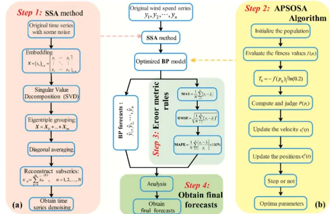
2. Methodology

In this section, all of the algorithms involved in this work are described. The full list of algorithms to be discussed in this section is as follows: the singular spectrum analysis algorithm, an efficient technology for time series analysis; the particle swarm optimization algorithm; the simulated annealing algorithm, which overcomes PSO falling into the local minima, and the back propagation neural network. The hybrid algorithm-APSOSA, raised to search for the optimal parameters of BPNN, will also be introduced in detail.

2.1. Singular Spectrum Analysis

(4)

series analysis. It was developed by Broomhead and King in 1986 [43]. Figure1shows the decomposed series of wind speed by SSA. The details are shown in AppendixA.1.

Figure 1._{Figure 1.} Original wind speed series and the decomposed series by SSA. _{Original wind speed series and the decomposed series by SSA.}

2.2. Intelligent Optimization Algorithms

In this section, several optimization algorithms will be introduced.

2.2.1. Particle Swarm Optimization

Inspired by imitating the social behavior of flocks of bird and schools of fish, an effective approach for optimization, Particle swarm optimization (PSO), was first developed by Dr. Eberharts and Dr. Kennedy in 1995 [44]. It is a stochastic, population-based evolutionary algorithm, which involves searching for solutions [39] (details in AppendixB.1).

2.2.2. Back Propagation Neural Network

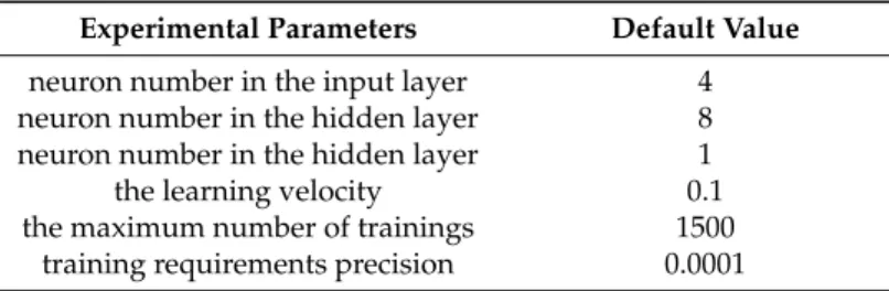
First proposed by Rumelhart and McCelland (1986) [45], the Back Propagation Neural Network (BPNN) is one of the most widely employed artificial neural network (ANN) models (details in AppendixB.2). It is not only capable of learning and storing a large amount of input–output mode mappings without needing to reveal the mathematical equations of the mapping relationship, but can also apply the steepest descent method, by back propagation, to constantly adjust the network weights and thresholds, resulting in the minimum square error. In addition, BPNN [46] consists of three layers: the input layer, the hidden layer, and the output layer. The experimental parameters are listed in Table1.

Table 1.The experimental parameters of BPNN.

Experimental Parameters Default Value

neuron number in the input layer 4 neuron number in the hidden layer 8 neuron number in the hidden layer 1

the learning velocity 0.1

(5)

2.2.3. Simulated Annealing

The concept of Simulated Annealing was first introduced by N. Metropolis et al. in 1953. In 1983, Kirkpatrick et al. succeeded in introducing SA in the field of combinatorial optimization [47]. Based on the Monte-Carlo iteration solving method, currently the SA algorithm has become one of the most popular heuristic random search methods. Unlike the PSO algorithm, SA can jump out of the trap of local minima in a timely manner to update the solutions and obtain the global optimum (details in AppendixB.3).

2.2.4. The Proposed Optimization Algorithm, APSOSA

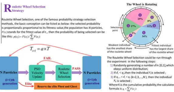
This paper proposes a hybrid APSO algorithm by employing the SA algorithm to prevent the PSO from falling into local minima (the algorithm of SA-APSO is shown in Table2). The major steps of the hybrid optimization algorithm are as follows. First, enhance the accuracy and convergence rate of the basic PSO algorithm by applying a compression factor and selecting suitable parameters. Next, by combining the Simulated Annealing characteristics, PSO can more easily and quickly obtain the optimal solution in a larger search space. SA can also cancel the restrictions on speed border. Moreover, the Roulette Wheel Selection Strategy is chosen, shown in Figure2, in this algorithm.

PSO can obtain better results in a faster setting with fewer parameters and is cheaper than other methods. It is also currently being widely used for promising results in continuous problems. However, the movement directionality of the particles is not certain, and particles are likely to jump out to obtain near-optimal solutions and their local search ability is relatively weak and easily trapped by the local optimum. Therefore, PSO is combined with the simulated annealing algorithm. The annealing algorithm is used when poor quality is probable to temporarily accept some solution features to construct a particle swarm algorithm, based on simulated annealing. A multitude of papers have verified that the improved particle swarm optimization algorithm obtains better results and have documented the effectiveness of the method through experimental simulation results. The velocity and position updating formula are as follows:

vi,jpk`1q “χrvi,jpkq `c1r1ppi,jpkq ´xi,jpkqq `c2r2ppg,jpkq ´xi,jpkqqs (1)

xi,jpk`1q “xi,jpkq `vi,jpk`1q,j“1, ...,n (2) wherer₁andr₂are set randomly between 0 and 1, and the learning factorsc₁andc₂are positive numbers, whereχis computed by the following formula:

χ“ ˇ 2 ˇ

ˇ2´C´

?

C2´4Cˇˇ ˇ

, C“c1`c2, Cą4 (3)

In Equation (3), applying the best group positions, all particles fly to the best group positions, and then tend to the local minima solution if the best group positions are in the local minimum. Accordingly, this situation will cause the search dispersability and ability to become worse. To overcome this weakness, a new position p1g will be selected from among the pi to replace pg.

Finally, in this paper, the Equation (1) is rewritten as the following formula, Equation (4):

vi,jpk`1q “χrv_i_,jpkq `c₁r₁pp_i_,_jpkq ´x_i_,jpkqq `c₂r₂pp1_i_,jpkq ´x_i_,jpkqqs (4)

However, how to address the suitable positionpiis one of the most critical steps of the combined

algorithm. Clearly, better performance of pi shall be considered a higher priority. Under the

characteristics of the SA algorithm, the best solutions of every particle pi should be taken as the

special one, which may be worse than the global optimal solution pg. Therefore, in the case of

temperatureT, we can calculate the leap probability using Equation (5):

(6)

whereFis the objective function value of the particle position.

The leap probability can be computed by the following formula, Equation (6):

Pppiq “

e´pFppiq´Fppgqq{KT N

ř

j“1e

´pFppiq´Fppgqq{KT

(6)

whereNis the population, on the side; considering the Roulette Wheel Selection strategy, we can randomly choose thepi, which will be regarded asp1g.

The chief steps of the APSOSA algorithm are as follows, and a flowchart is depicted in Figure2.

Step 1: Set the initial temperature, and initialize the population along with every particle velocity and position.

Step 2: ComputeFppiq pi“1, ..,Nq, whereNis the updated population.

Step 3: Update the present position and fitness value of each particle by using pi, Fppiqand pg, Fppgq, respectively.

Step 4: Compute the initial temperature using Equation (7):

T₀“ ´Fppgq{lnp0.2q (7)

Step 5: Update the particle position and velocity and computePppiq.

Step 6: Through the roulette wheel selection strategy, the new global optimal solutionp1gis not regarded

aspguntilPppiq ąrandp q.

Step 7: Update every particle velocity and position by the pre-set update formula.

Step 8: Compute every particleFpp1_iq, and then do not apply piFppiqto update the current global

positionpgand optimal fitness valueFppgq, respectively, untilFppiq>Fppgq.

Step 9: By applying the pre-set rules, the temperature reduces slowly.

Step 10: Analyze whether the pre-set conditions are met; if they have been met, output the information ofpgand then end running. Otherwise, repeat the above steps, beginning with Step 5.

 



 

 





 

 







(7)

Table 2.A rudimentary SA-APSO algorithm is outlined as follows.

Algorithm:SA-APSO

Input:

xps0q“

´

xp0qp1q,xp0qp2q, . . . ,xp0qplq¯–a sequence o f training data.

xpp0q“

´

xp0qpl`1q,xp0qpl`2q, . . . ,xp0qpl`nq¯–a sequence o f veri f ying data.

Output:

Pg—the value of x with the best fitness value in population of particles Parameters:

Itermax—the maximum number of iterations

n—the number of particles

Fi—the fitness function of particlei

xi—particlei

g—the current iteration number d—the number of dimension

1: /* Set the parameters of PSO and SA. */

2: /* Initialize population ofnparticlexi(i= 1, 2,...,n) randomly */ 3:FOR EACHi: 1ďiďnDO

4: Evaluate the corresponding fitness functionFi 5:END FOR

6: /* Determine the global best position */ 7:FOR EACHi: 1ďiďnDO

8: Determine the global best positionPgby usingF(xi). 9: {F(Pg),g}=max{(F(P1), . . . ,F(PN)}

10:END FOR

11:WHILE(g<Itermax)DO

12: /* Determine the initial temperature. */ 13:FOR EACHi: 1ďiďnDO

14:T0=´F(Pi)/ln(0.2) 15:END FOR

16:FOR EACHi =1:nDO

17:FOR EACHj= 1:nDO

18: /* Calculate the probabilityP(Pi) */

19: /* Judge the relationship of the probabilityP(P_i) and rand () */ 20:IF(P(Pi) > rand())THEN

21:Pg=P1g=Pi 22:END IF

23: /* Update the velocity and position of each particle */ 24:FOR EACHi: 1ďiďnDO

25:vi(t + 1) = w(t)vi(t) + c1r1(pi´xi(t)) + c2r2(pg´xi(t)); 26:x_i(t + 1)=x_i(t) +v_i(t + 1);

27:END FOR

28: /* Evaluate the new positionP1iand fitness functionF(P1i). */ 29:FOR EACHi: 1ďiďnDO

30: Evaluate the corresponding fitness functionF(P1_i) 31:END FOR

32: /* Judge the relationship of fitness functionF(P1i) andF(Pi). */ 33:IF(F(P1_i) >F(P_i))THEN

34:Pi=P1iandF(Pi) =F(P1i) 35:END IF

36: /* Judge the relationship of fitness functionF(Pi) andF(Pg). */ 37:IF(F(P_i) >F(Pg))THEN

38:Pg=PiandF(Pg) =F(Pi) 39:END IF

40: /* Cooling the temperature */ 41:FOR EACHi: 1ďiďnDO

42:Ti + 1=aˆTi 43:END FOR

44:END FOR

45:END FOR

46:END WHILE

(8)

2.2.5. SSA–APSOSA–BPNN Algorithm

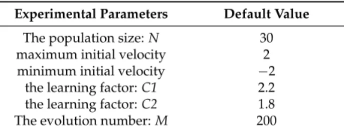
In this section, we will introduce the hybrid model (SSA–APSOSA–BPNN) more clearly. The flowchart of the model is described in Figure3. And the experimental parameters of APSOSA are given in Table3. The hybrid algorithm contains four main stages.

Table 3.The experimental parameters of APSOSA.

Experimental Parameters Default Value

The population size:N 30

maximum initial velocity 2

minimum initial velocity ´2

the learning factor:C1 2.2

the learning factor:C2 1.8

The evolution number:M 200

Stage I: Data prepossessing. Utilize the SSA method to process the original wind speed signals; as a result, the noise signals are removed, and the real and effective signals, which are shown in Figure1, can be preserved. Lastly, the useful processed signal will be fed into the abovementioned hybrid model.

Stage II: Data selection. The processed valid data from Stage I is classified into three parts: the training set, the validation set, and the test set for model training, validation, and testing, respectively. Stage III: Algorithm training and validation. Here, the SSA–APSOSA–BPNN algorithm is utilized for wind speed forecasting. Additionally, the detailed rules are given as below:

Step 1: Determine and initialize the parameters of APSOSA.

Step 2: Set the fitness function; the mean absolute error (MAE) of validation is taken as the fitness of the particles:

f itness“MAE“ _N1 N

ÿ

i“1

|yi´yˆi| (8)

whereNis the number of validation sets and ˆyiandyistand for the predictive value and the observed

value, respectively.

Step 3: Update the historical extremum pj of every particle and the global extremum pgand then

repeat the above rules for the next particles.

Step 4: Set the conditions and judge whether the fitness value meets the conditions; if it does, save the corresponding optimal parameters and then stop running. Otherwise, run Step 3 again and continue to run.

(9)

Figure 3. The flowchart of the proposed hybrid algorithm. Figure 3.The flowchart of the proposed hybrid algorithm.

3. Case Study

To examine the accuracy of the novel combined algorithm, four different multi-step forecasting algorithms are compared by analyzing the three-step-ahead-prediction (half–1-h-ahead) and the six-step-ahead-prediction (1-h-ahead) of a 10-min wind speed series at three different wind power stations.

3.1. Study Area and Datasets

Shandong, located on the east coast of China, is not only one of the provinces with the largest economy, but also one of the biggest energy consumers. However, 99% of the electrical energy comes from coal power generation. As a result, Shandong faces enormous energy pressures.

(10)

Figure 4.The study area, Penglai in Shandong province, eastern China.

In this work, Penglai, which is located north of Shandong and lies north of the Yellow Sea and the Bohai Sea, was chosen as the area of study. It has tremendous, potentially valuable wind resources. The specific advantages are as follows: (i) higher elevation but relatively flat hilltops, ridges, and a special terrain that has much potential as an air strip; (ii) longer cycle of efficient power generation; (iii) suitable climatic conditions that are conducive to the normal operation of wind turbines; and (iv) small diurnal and seasonal variations of wind speed, which can reduce the impact on power.

In this study, the 10-min wind speed data from Penglai wind farms are used to obtain a detailed example for evaluating the performance of the proposed model. First, the wind speed data are divided into four parts according to the seasons, so that the impact of seasonal variations can be considered to increase the stability of the proposed model. Next, every seasonal wind speed dataset is divided into three parts: a training set, a validation set, and a testing set. Additionally, the noise is removed from the data by using SSA. Finally, the processed data are entered into the model and, judging from the forecasting results, we determine whether the raised algorithm can be widely employed for real-world farm use. In this study, the experiment is applied to three different sites (Site 1, 2, and 3). The above-described experiment is scientific and is used to validate the performance of the proposed model.

3.2. Performance Criteria of Forecast Accuracy

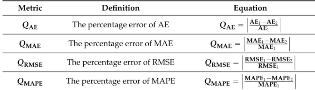
To evaluate the prediction accuracy of the raised hybrid algorithm, four indexes are applied to measure the quality of the forecasting methods: absolute error (AE), mean absolute error (MAE), root mean square error (RMSE), and mean absolute percent error (MAPE), shown in Table4(here Nis the number of test samples, and ˆyiandyi represent the real and forecast values, respectively).

(11)

the credibility of the forecasting model. Wind speed forecasting errors are related to not only the forecasting models but the selected samples. Consequently, the forecasting errors within a certain scientific range can be accepted. Moreover, in order to better evaluate performance, four percentage error criterions are also applied in this study, listed in Table5.

Table 4.Four metric rules.

Metric Definition Equation

AE The average forecast error ofitimes forecast results AE“ _N1 řN

i“1pyi´yˆiq

MAE The average absolute forecast error ofitimes forecast results MAE“_N1 řN

i“1|yi´yˆi|

RMSE The root average of the prediction error squares RMSE“

d

1 N

N

ř

i“1pyi´yˆiq 2

MAPE The average of absolute error MAPE“ _N1 řN

i“1

ˇ ˇ ˇ

yi´yˆi

yi ˇ ˇ ˇˆ100%

Table 5.Four metric rules.

Metric Definition Equation

Q_AE The percentage error of AE QAE“

ˇ ˇ ˇ

AE1´AE2

AE1

ˇ ˇ ˇ

QMAE The percentage error of MAE QMAE“ ˇ ˇ ˇ

MAE1´MAE2

MAE1

ˇ ˇ ˇ

Q_RMSE The percentage error of RMSE Q_RMSE“ˇˇ ˇ

RMSE1´RMSE2

RMSE1

ˇ ˇ ˇ

QMAPE The percentage error of MAPE QMAPE“ ˇ ˇ ˇ

MAPE1´MAPE2

MAPE1

ˇ ˇ ˇ

3.3. Experimental Simulations

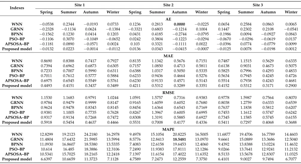
In this subsection, three single models, WNN, GRNN, and BPNN, are compared to obtain the best prediction approach. As a result, whether for half-hour (rolling three-step) or one-hour (rolling six-step) predictions, BPNN gives the best prediction accuracy (see Tables6and7) of the four proposed models. Next, the APSOSA-BPNN is selected from BPNN, PSO-BPNN as the best prediction algorithm. Finally, the hybrid SSA–APSOSA–BP algorithm was proposed as our best prediction model.

(12)

Table 6.Comparison of errors of rolling three-step (half an hour ahead) forecasts.

Indexes Site 1 Site 2 Site 3

Spring Summer Autumn Winter Spring Summer Autumn Winter Spring Summer Autumn Winter

AE

WNN ´0.0538 0.2344 ´0.0193 0.0733 0.1236 0.2813 0.0000 ´0.0225 0.0654 0.2584 0.0863 0.0065

GRNN ´0.2328 ´0.1134 0.0624 ´0.1384 ´0.3321 0.6803 ´0.1214 0.1004 0.1447 0.2302 0.2108 ´0.0541

BPNN ´0.1562 0.1230 0.0414 0.1203 0.0431 0.4185 ´0.2744 ´0.0795 ´0.1986 0.0094 ´0.0927 0.0843

PSO–BP ´0.1106 0.3070 ´0.1049 ´0.0652 0.0242 0.3804 ´0.1223 ´0.0294 ´0.0670 ´0.0296 ´0.0619 0.0137

APSOSA–BP ´0.1181 0.0890 ´0.0571 0.0024 0.103 0.3321 ´0.1111 0.0022 ´0.0396 0.0774 ´0.0779 0.0099

Proposed model ´0.0132 0.0223 ´0.0014 ´0.0112 0.0136 0.0343 ´0.0415 ´0.0007 ´0.0125 0.0078 ´0.0198 0.0012

MAE

WNN 0.8690 0.8388 0.7417 0.7927 0.8135 1.1342 0.5676 0.7151 0.7487 1.1515 0.5629 0.6335

GRNN 0.7394 0.6962 0.6873 0.6305 0.7157 1.0850 0.4713 0.5811 0.6138 0.9031 0.4673 0.5075

BPNN 0.7233 0.7007 0.5990 0.6311 0.6388 1.0317 0.5050 0.5335 0.5825 0.7996 0.4293 0.4833

PSO–BP 0.7011 0.7612 0.5777 0.5884 0.6233 0.9436 0.4664 0.5276 0.5634 0.7945 0.4245 0.4726

APSOSA–BP 0.6975 0.6545 0.5549 0.5761 0.6230 0.9133 0.4571 0.5143 0.5514 0.7938 0.4243 0.4681

Proposed model 0.4493 0.4151 0.3437 0.3489 0.4211 0.5312 0.3289 0.3351 0.4152 0.5312 0.3171 0.2900

RMSE

WNN 1.1530 1.1683 0.9791 1.0244 1.0591 1.5757 0.7316 0.9383 0.9778 1.5987 0.7564 0.8070

GRNN 0.9784 0.9479 0.9999 0.8147 0.9165 1.6059 0.6052 0.7680 0.8038 1.2759 0.6333 0.6539

BPNN 0.9624 0.9478 0.8343 0.8145 0.8454 1.6364 0.6543 0.7169 0.7637 1.1838 0.5812 0.6207

PSO–BP 0.9381 1.1005 0.7735 0.7628 0.8267 1.3967 0.6005 0.6995 0.7453 1.1612 0.5747 0.6242

APSOSA–BP 0.9317 0.9134 0.7268 0.7472 0.8308 1.3191 0.5885 0.6927 0.7345 1.1585 0.5745 0.6155

Proposed model 0.5918 0.5454 0.4637 0.4466 0.5531 0.7008 0.4177 0.4336 0.5411 0.7297 0.4068 0.3688

MAPE

WNN 12.8299 19.2123 24.2180 16.2978 9.4978 15.1054 20.8225 16.5005 11.6877 19.4706 16.7789 14.4603

GRNN 11.4804 17.6432 21.5985 13.5994 8.5776 12.8413 18.5481 13.0970 9.6661 15.0889 13.3686 12.5040

BPNN 11.0930 16.8607 18.5380 13.5335 7.4083 12.6158 19.6453 12.4060 9.4392 13.8388 13.0224 11.4632

PSO–BP 10.614 16.485 18.3886 12.3106 7.2490 11.9383 17.8111 12.1286 9.0266 13.7641 12.9241 11.2132

APSOSA–BP 10.5341 15.7025 18.2165 12.2418 7.1397 11.6154 17.4022 11.6352 8.5133 13.5678 12.8307 11.0325

(13)

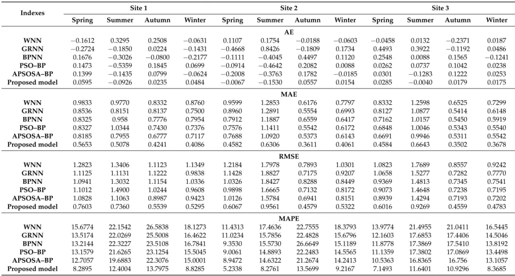
Table 7.Comparison of errors of rolling six-step (one hour ahead) forecasts.

AE

WNN ´0.1612 0.3295 0.2508 ´0.0631 0.1107 0.1754 ´0.0188 ´0.0603 ´0.0458 0.0132 ´0.2371 0.0187

GRNN ´0.2724 ´0.1850 0.0224 ´0.1431 ´0.4668 0.8426 ´0.1809 0.1734 0.4493 0.3922 ´0.1192 0.0486

BPNN 0.1676 ´0.3026 ´0.0800 ´0.2177 ´0.1111 ´0.4045 0.4497 0.1120 0.2548 0.0088 0.1565 ´0.1241

PSO–BP 0.1473 ´0.5359 0.1845 0.0699 ´0.0914 ´0.4642 0.2082 0.0088 0.0262 0.0737 0.1042 0.0238

APSOSA–BP 0.1399 ´0.1435 0.0799 ´0.0624 ´0.2008 ´0.3763 0.1782 ´0.0185 0.0301 ´0.1283 0.1222 0.0253

Proposed model 0.0595 ´0.0926 0.0235 0.0484 ´0.0067 ´0.1530 0.0557 0.0154 0.0285 ´0.0040 0.0179 0.0175

MAE

WNN 0.9833 0.9770 0.8332 0.8760 0.9599 1.2853 0.6176 0.7797 0.8332 1.2598 0.6525 0.7299

GRNN 0.8536 0.8151 0.8137 0.7500 0.8960 1.2891 0.5554 0.6993 0.8127 1.0877 0.5414 0.6148

BPNN 0.8325 0.958 0.7776 0.7954 0.7912 1.1887 0.6559 0.6417 0.7162 1.0157 0.5450 0.5919

PSO–BP 0.8327 1.0344 0.7430 0.7376 0.7576 1.1411 0.5542 0.6172 0.6848 1.0046 0.5343 0.5540

APSOSA–BP 0.8185 0.7955 0.6777 0.7117 0.7688 1.0920 0.5373 0.6143 0.6691 0.9946 0.5311 0.5542

Proposed model 0.5653 0.5078 0.4241 0.4086 0.4582 0.6306 0.3611 0.4061 0.4584 0.6643 0.3502 0.3678

RMSE

WNN 1.2823 1.3406 1.1123 1.1349 1.2184 1.7978 0.7893 1.0301 1.0823 1.7689 0.8557 0.9242

GRNN 1.1125 1.1131 1.1222 0.9838 1.1428 1.8827 0.7175 0.9207 1.0658 1.5277 0.7282 0.7770

BPNN 1.0941 1.3032 1.1154 1.0336 1.0326 1.8427 0.8288 0.8449 0.9369 1.4813 0.7345 0.7541

PSO–BP 1.1012 1.4900 1.0244 0.9608 0.9898 1.6665 0.7132 0.8172 0.9073 1.4648 0.7238 0.7195

APSOSA–BP 1.0828 1.1063 0.8987 0.9423 1.0126 1.5784 0.6941 0.8151 0.8939 1.4294 0.7193 0.7202

Proposed model 0.7603 0.7360 0.5539 0.5295 0.6067 0.9561 0.4579 0.5322 0.6016 0.9269 0.4559 0.4783

MAPE

WNN 15.6774 22.1542 26.5838 18.1273 11.4313 17.4636 22.7555 18.3793 13.9774 21.4955 21.0411 16.5445

GRNN 13.5174 22.0269 25.5008 16.4622 11.0234 15.7856 22.4828 15.6796 12.1603 17.6853 17.4406 14.5046

BPNN 13.2144 22.3227 23.5108 16.7841 9.3530 15.5730 26.6649 15.1189 11.8778 17.3869 17.5410 13.8192

PSO–BP 13.1579 21.6265 23.1254 15.5045 9.0061 14.8893 22.2483 14.5565 11.1359 17.3802 17.0869 13.4498

APSOSA–BP 12.7057 19.6883 22.3076 15.0001 8.9472 14.6322 21.2674 14.2413 10.5363 16.8365 16.756 13.1057

(14)

Table 8.Improvement percentages among different forecasting models of rolling three-step (half an hour ahead) forecasts.

QAE

BP vs. Proposed model 91.5470 81.8408 103.3182 109.3035 68.3453 91.7930 84.8808 99.1144 32.0906 34.9459 25.1336 41.4849

PSO vs. Proposed model 88.0618 92.7230 98.6902 82.8185 43.6765 90.9706 66.0777 97.6089 28.9866 34.5929 24.5642 40.1803

APSOSA vs. Proposed model 88.8219 74.9061 97.5929 564.8312 86.7541 89.6562 62.6562 131.4576 24.7049 33.6466 24.0151 39.2005

QMAE

QRMSE

QMAPE

Table 9.Improvement percentages among different forecasting models of rolling six-step (one hour ahead) forecasts.

QAE

PSO vs. Proposed model 59.5977 82.7136 87.2727 30.7280 92.6464 67.0416 73.2619 74.6921 35.7995 33.0267 36.0352 37.7797 APSOSA vs. Proposed model 57.4865 35.4692 70.6258 177.6135 96.6529 59.3472 68.7603 183.3262 32.1460 30.8639 34.7720 36.1461

QMAE

QRMSE

BP vs. Proposed model 30.5091 43.5236 50.3407 48.7713 41.2454 48.1142 44.7514 37.0103 35.7882 37.4266 37.9306 36.5734 PSO vs. Proposed model 30.9571 50.6040 45.9293 44.8897 38.7048 42.6283 35.7964 34.8752 33.6934 36.7217 37.0130 33.5233

QMAPE

(15)

(16)

From Tables6and7, we can see following:

(a) Different forecasting algorithms have different forecasting results;

(b) All the algorithms’ forecasting results from the three sites are effective. Examples are included in Figure5;

(c) For different seasons at the same site, the hybrid algorithms show strong forecasting stability; (d) Among the algorithms studied, the hybrid SSA–PSOSA–BP algorithm (see in Figure6) obtained

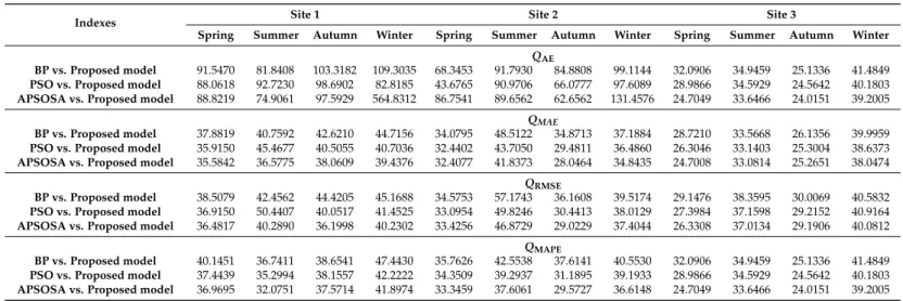
better accuracy than the others. Moreover, to further illustrate the quality of the proposed hybrid algorithm, four percentage error criterions are used in Table5.

It can be analyzed in detail that:

(a) When comparing the hybrid PSO–BP algorithm with the single BP algorithm, we can make a conclusion that the PSO selects excellent parameters to run BP model, but the prediction accuracy of PSO–BP is increased only slightly. From Tables6and7, in the spring, the three-step MAPE results of the PSO–BP and the BP are 7.2490% and 7.4083%, respectively. For the six-step, they are 9.0061% and 9.3530%, respectively.

(b) When comparing the hybrid PSOSA–BP algorithm with the combined PSO–BP algorithm,

the former combines the advantages of simulated annealing, and further optimizes the parameters; as a result, with respect to (a), the predicted quality rises again, but not particularly clearly. The specific upgrade percentages are provided in Tables8and9.

(c) When comparing the hybrid SSA–APSOSA–BP algorithm with the hybrid PSOSA–BP algorithm, the former MAPE results are better than the latter. In other words, the forecasting quality of the new combined algorithm is better because of the higher accuracy when comparing it with the BP, PSO–BP, and PSOSA–BP algorithms.

(d) The forecasting quality of the hybrid SSA–APSOSA–BP algorithm is better than that of the hybrid PSO–BP algorithm. The decreases in MAPE results in comparison with the PSO–BP and SSA–APSOSA–BP algorithm of three-step and six-step forecasts are 37.4439% and 36.9998% in Tables8and9for the spring season, respectively.

(e) When comparing the hybrid SSA–APSOSA–BP algorithm with the single BP algorithm, the accuracy of the wind speed forecasting, is improved more obviously. As an example, in Table6, the three-step forecasting MAPE results for the latter are 9.4392%, 13.8388%, 13.0224%, and 11.4632%, respectively. However, for the former, the three-step forecasting MAPE results are 6.4101%, 9.0027%, 9.7494%, and 6.7077%, respectively.

(f) From (a) to (e), the reasons include:

(1) The combination of the SA algorithm and the PSO algorithm has increased the forecasting ability and accuracy of the single BP algorithm effectively.

(2) The SSA algorithm removes the noise signal from the original wind speed data and, due to the APSOSA algorithm, the best initial weights and thresholds are given to optimize the BP algorithm, which can lead to high-precision forecasting results.

(3) The scientific and rational data selection used in this paper is also one of the paramount reasons for the outstanding performance achieved.

In different seasons at the same site, the proposed algorithms’ forecasting qualities can also be different. This phenomenon indicates that wind speed can be affected by seasonal factors. In this paper, we also consider this factor, and the different seasons’ forecasting results are listed in Tables6and7. Tables 10and11are chosen as examples, and the detailed descriptions of this phenomenon are as follows:

(17)

(b) In Table11, for the hybrid SSA–APSOSA–BP algorithm in spring and winter, the MAPE of the three-step and six-step are 5.9362% and 6.8909% vs. 7.0652% and 8.8046%, respectively. However, in summer and autumn, they are 8.9720% and 10.7722% vs. 11.1259% and 12.7657%, respectively. Obviously, in spring and winter, the MAPE results are less than 9%, but in summer and autumn, the wind speed forecasting errors are all more than 10%, especially in autumn when they are close to 12%.

(c) As can be clearly observed from the circumstances described above, geographical and seasonal factors must be considered in the wind speed prediction. From (b), it can be concluded that the prediction accuracy in spring and winter is better than that in summer and autumn. However, comparing with the other proposed algorithms, the forecasting errors of the hybrid algorithm are still effectively less.

Table 10.Average errors of the different rolling forecasting models at the three sites.

BP PSO–BP APSOSA–BP SSA–APSOSA–BP

Area Average 3-Step 6-Step 3-Step 6-Step 3-Step 6-Step 3-Step 6-Step

Site 1

AE (m/s) ´0.0321 ´0.1082 ´0.0066 ´0.0336 0.0210 0.0035 0.0009 0.0097 MAE (m/s) 0.6635 0.8409 0.6571 0.8369 0.6208 0.7509 0.3893 0.4765 RMSE (m/s) 0.8898 1.1366 0.8937 1.1441 0.8298 1.0075 0.5119 0.6449 MAPE (%) 15.0063 18.9580 14.4496 18.3536 14.1737 17.4254 8.9477 10.8290

Site 2

AE (m/s) ´0.0269 0.0115 ´0.0632 ´0.0847 ´0.0816 ´0.1044 ´0.0014 ´0.0222 MAE (m/s) 0.6773 0.8194 0.6402 0.7675 0.6269 0.7531 0.4041 0.4640 RMSE (m/s) 0.9633 1.1373 0.8809 1.0467 0.8578 1.0251 0.5263 0.6382 MAPE (%) 13.0189 16.6775 12.2818 15.1751 11.9481 14.7720 7.9093 9.0741

Site 3

AE (m/s) 0.0494 0.0740 0.0362 0.0570 0.0076 0.0123 0.0058 0.0150 MAE (m/s) 0.5737 0.7172 0.5638 0.6944 0.5594 0.6873 0.3884 0.4602 RMSE (m/s) 0.7874 0.9767 0.7764 0.9539 0.7708 0.9407 0.5116 0.6157 MAPE (%) 11.9409 15.1562 11.7320 14.7632 11.4861 14.3086 7.9675 9.5219

Table 11.Average errors of the different rolling forecasting models in different seasons.

BP PSO–BP APSOSA–BP SSA–APSOSA–BP

Season Average 3-Step 6-Step 3-Step 6-Step 3-Step 6-Step 3-Step 6-Step

Spring

AE (m/s) 0.1039 0.1038 0.0511 0.0274 0.0182 ´0.010 0.0040 0.0271 MAE (m/s) 0.6482 0.7800 0.6293 0.7584 0.6240 0.7521 0.4285 0.4940 RMSE (m/s) 0.8572 1.0212 0.8367 0.9994 0.8323 0.9964 0.5620 0.6562 MAPE (%) 9.3135 11.4817 8.9632 11.100 8.7290 10.729 5.9362 6.8909

Summer

AE (m/s) ´0.1836 ´0.2328 ´0.2193 ´0.3088 ´0.166 ´0.2160 ´0.021 ´0.083 MAE (m/s) 0.8440 1.0541 0.8331 1.0600 0.7872 0.9607 0.4925 0.6009 RMSE (m/s) 1.2560 1.5424 1.2195 1.5404 1.1303 1.3714 0.6586 0.8730 MAPE (%) 14.4384 18.4275 14.0625 17.965 13.628 17.0523 8.9720 10.772

Autumn

AE (m/s) 0.1086 0.1754 0.0964 0.1656 0.0820 0.1268 0.0209 0.0324 MAE (m/s) 0.5111 0.6595 0.4895 0.6105 0.4788 0.5820 0.3299 0.3785 RMSE (m/s) 0.6899 0.8929 0.6496 0.8205 0.6299 0.7707 0.4294 0.4892 MAPE (%) 17.0686 22.5722 16.3746 20.8202 16.1498 20.1103 11.1259 12.7657

Winter

(18)

(19)

4. Discussion

In this section, the bias–variance framework and the Diebold–Mariano (DM) are used to examine the accuracy, the stability, and the forecasting performance of the forecast models.

4.1. Bias–Variance Framework

In order to evaluate the different models’ accuracy and stability, in this subsection, we utilize the bias–variance framework, which includes bias and variance. The bias-variance framework can be shown as follows:

var“Erpyˆýq Épyˆýqs2 (9)

Bias2“Eryˆýs2ÉryˆÉpyˆq2s (10) whereyand ˆyare the observed values and the forecasting values respectively.

The higher the bias, the lower the forecasting accuracy. Similarly, the bigger the variance, the worse the prediction performance. The results of the models are shown in Tables12and13. Obviously, the bias and variance of the proposed hybrid model are smaller than the comparison models (GRNN, WNN, APSOSA–BPNN, etc.). In other words, the developed model possesses a higher accuracy and stability in wind-speed forecasting and performs much better than the comparison models in forecasting.

Table 12.Bias–variance and Diebold–Mariano test of different models (half an-hour ahead).

Different Models Bias–Variance Framework Diebold–Mariano Statistic

Bias2 _Var

WNN 0.019750 1.186340 15.016983 *

GRNN 0.067441 0.849879 12.978130 *

BPNN 0.030799 0.820297 13.903475 *

PSO–BP 0.024353 0.758024 13.244862 **

APSOSA–BP 0.014342 0.706074 12.841336 **

Proposed model 0.000375 0.278953 —

* is the 1% significance level; ** is the 5% significance level.

Table 13.Bias–variance and Diebold–Mariano test of different models (one hour ahead).

Different Models Bias–Variance Framework Diebold–Mariano Statistic

Bias2 Var

WNN 0.025612 1.497107 16.081645 *

GRNN 0.124355 1.170295 13.999003 *

BPNN 0.055763 1.211757 12.749358 *

PSO–BP 0.052717 1.144234 12.080501 **

APSOSA–BP 0.024791 1.029058 12.739267 **

Proposed model 0.003605 0.424805 —

* is the 1% significance level; ** is the 5% significance level.

4.2. Statistical Hypothesis Testing

(20)

In this subsection, another hypothesis testing approach is employed to assess the models’ efficiency, called the Diebold–Mariano test [10]. The concrete content is described as follows:

H0:ErpLpe_t1qs “ErpLpe2_tqs

H₁:ErpLpe_t1qs ‰ErpLpe2_tqs

where the Loss functionLis the function of the prediction error,e1_t ande2_t are the forecasting errors of the two comparison models.

Establishing the DM Statistics:

DM“b d

2πfˆ_dp0q N

d

ÑNp0, 1q (11)

d“ 1 N

N

ÿ

t“1

rLpe1_tq ´Lpe2_tqs (12)

where 2πfˆdp0qrepresents a consistent estimator of the asymptotic variance, ˆfdp0qis the zero spectral density, andNis the length of forecasting results.

Comparing the calculated DM with theZ_α{₂, which can be found in the normal distribution table, the null hypothesis will be rejected ifˇˇ

ˇDM ˇ ˇ ˇą

ˇ ˇ ˇZα{2

ˇ ˇ

ˇ; this means that under the significance levelα, there is a significant difference between the two models (the proposed model and the compared models including WNN, GRNN, BPNN, etc.) in terms of their prediction performance. The concrete results are shown in Tables12and13.

4.3. Analysis

From Tables12and13, we can see that:

(a) No matter the bias or the variance, the values of the proposed model are far smaller than those of the other five models, which means that the hybrid model has a higher accuracy and stability than the other five models.

(b) The smallest value of the|DM|in both tables is 12.080501, which is much larger than theZ_α{₂ (Z0.005“2.58,Z0.025“1.96); as a consequence, the null hypothesis can be rejected and the hybrid model observably outperforms the other five models.

5. Conclusions

With the conventional energy for electricity generation being quickly depleted, wind energy has become the most significant new type of green renewable energy available, and contains enormous power. However, due to the uncertainty of meteorological factors, it is still an extremely challenging task to forecast wind speed. In this paper, we put forward a novel hybrid SSA–APSOSA–BP model based on SSA and simulated annealing—adaptive particle swarm optimization algorithm (the specific process is given in Figure6). From the above discussion and analysis, the conclusions are expressed as follows:

(1) Among the three single prediction methods (WNN, GRNN, and BPNN), the best one is BPNN, which possesses a stronger prediction performance than the others (see Tables6and7).

(2) In summer and autumn, wind speed forecasting errors are larger than in another two seasons because of the more complex features of wind speed in Penglai.

(21)

and credible within a reasonable range. The detailed reasons are provided in the above experimental simulations Section3.3.

Overall, the proposed hybrid model adds a new viable option for wind speed forecasting, and the excellent performance and reasonable prediction accuracy reveal that they can be employed for time series forecasting, especially for wind-speed forecasting in some cases.

Acknowledgments:This work was financially supported by the National Natural Science Foundation of China (71171102).

Author Contributions: Pei Du and Yu Jin conceived and designed the experiments; Pei Du performed the

experiments; Pei Du and Yu Jin analyzed the data; Kequan Zhang contributed reagents/materials/analysis tools; Pei Du wrote the paper.

Conflicts of Interest:The authors declare no conflict of interest.

Appendix A

Appendix A.1 Singular Spectrum Analysis (SSA)

Standard SSA is made up of two stages, decomposition and reconstruction, and each stage contains two steps.

Given a one-dimensional time seriespy₁,¨ ¨ ¨ ,yNqof lengthN, whereL(integer) is the window lengthLp1ăLăNq, andKis the number of lagged vectorspK“N´L`1q, the specific steps are as follows:

Stage 1: Decomposition

In this stage, there are two steps: embedding and singular value decomposition (SVD).

Step 1: Embedding.

Form the trajectory matrix of the seriesX_px1,¨ ¨ ¨ ,xKq, which can be expressed by:

X“ » — — — — — — –

y1 y2 y3 ¨ ¨ ¨ yk y2 y3 y4 ¨ ¨ ¨ yk`1 y3 y4 y5 ¨ ¨ ¨ yk`2

..

. ... ... ... ...

yL yL`1 yL`2 ¨ ¨ ¨ yN

fi ffi ffi ffi ffi ffi ffi fl LˆK (A1)

what is noteworthy is thatTij, an element ofX, stands for thei-th line and thej-th column, which

possess the characteristicTij“Ti´1,j`1.

Step 2: SVD

Calculate the matrixSpS“XXTqand the eigenvaluesλ1, ...,λL. ofS, which are the decreasing

sequence λ1 ě ... ě λL ě 0. Furthermore, U1, ... ,UL represent the corresponding orthogonal

eigenvectors of the matrixS. Lastly, theSVDof the trajectory matrixXcan be expressed through

Equation (A2):

X“X₁`...`Xd (A2)

whereXi “

a

λiUivTi having rank 1,d “ ti, such that λi ą0uandvi “XTUi{

a

λi pi“1, ...,dqare

elementary matrices. The grouppa

λi,Ui,vTiqwill be known as thei-th eigentriple (abbreviated asET).

Stage 2: Reconstruction

(22)

Step 3: Grouping

Firstly, we divide the abovementioned matrixXiintomgroups, which are different from each

other, and then add up the total matrices in each group. Next, letI “ i₁, ...,ip(,i1, ...,ipstand for

the indices of each group, and then theI-th group resultant matrixXI can be described as below: XI “ Xi₁`...`Xip. Here, we divideI “ t1, ...,duinto two different subsets I1 “ t1,¨ ¨ ¨ ,ru, and I₁“ tr`1,¨ ¨ ¨,du, thenXIcan be written as Equation (A3):

XI “XI1`...`XIm (A3)

Step 4: Diagonal Averaging

In this step, transform the mentioned grouped matrixXIinto a new series of lengthNand set X“ pxijq_L_ˆ_K, ifLąK, x˚_ij“xji, otherwisex˚ij“xij. Finally,pf1,¨ ¨ ¨,fNqcan be converted to a series by Equation (A4):

fk “

$ ’ ’ ’ ’ ’ ’ ’ & ’ ’ ’ ’ ’ ’ ’ % 1 k`1 k`1 ř

m“1ym,k´m`2 0ďkďL ˚_´₁

1 L˚

L˚ ř

m“1ym,k´m`2 L

˚_ď_k_ď_k˚

1 k`1

k`1 ř

m“1ym,k´m`2 k

˚_ď_k_ď_N_´₁

(A4)

in whichL˚“minpL,kq, k˚“maxpL,kq. In this method, the firstrmain constituents can be viewed as the most vital information, the rest are considered the noise of the original data.

Appendix B

Appendix B.1 Particle Swarm Optimization

The core of the PSO is learning the foraging behavior of birds. Assuming a forest setting, the birds do not know the position of the food. However, they can receive some information concerning the food location, and then search for the nearest food. These birds can be treated as the particles in the PSO algorithm; each particle can be regarded as a candidate solution in search space (ndimensions). Each particle continues to search for a better position by adjusting its velocityv_iptq “ rv1_i,v2_i, . . . ,vn_isT;

in light of their flying memory, birds decide on the personal best (pbest) solution. Finally, the global best (gbest) solution can be obtained by comparing the personal best solutions with each other. The updated position and velocity rules are defined as Equations (B1) and (B2):

vipt`1q “ωptqviptq `c1r1ppbest´xiptqq `c2r2pgbest´xiptqq (B1)

xipt`1q “xiptq `vipt`1q (B2)

where t is the current iteration, ω stands for the inertia weight, the particle position is xiptq “ rx1_i,x2_i,¨ ¨ ¨,xn_is, r1 andr2 are random numbers in [0, 1], and the learning factors c1 and c2 stand for weights ofpbestandgbest,respectively.

Appendix B.2 Back Propagation Neural Network (BPNN)

We determined the input vector by normalizing each input value by Equation (B3):

V“ tViu “ xi´ximin

ximax´ximin (B3)

(23)

Step 1: Calculate the outputs of all hidden layer nodes. Based on the input vectorX, the weightωij,

which is between the input layer and the hidden layer, and the hidden layer thresholdO, compute

outputsHof the whole hidden layer node in Equation (B4).Sis the number of the hidden layer nodes.

Hj “Gp n

ÿ

i“1

ωijxi´ajq, j“1,¨ ¨ ¨ ,s (B4)

Gpxq “₁ 1

`e´x (B5)

Step 2: Make a calculation about the output data of neural network, according to outputsHof all

hidden layer nodes, the weightsωij, and the weightλusing Equation (B6):

Ok“ l

ÿ

j“1

Hjωjk´λk, k“1, . . . ,p (B6)

Step 3: Depending on the predicted outputOand the expected outputY, calculate the error using

Equation (B7):

ek“Yk´Ok, k“1, . . . ,p (B7)

Step 4: Update the weights by using the predicted error and the weightsωijωjkin Equations (B8) and (B9):

ωij“ωij`ηHjp1´Hjqxi m

ÿ

k“1

ωikek, i“1, . . . ,n; j“1, . . . ,s (B8)

ωij“ωij`ηHjek,k“1, . . . ,p, j“1, . . . ,s (B9)

Step 5: Update the thresholds using Equations (B10) and (B11):

aj“aj`ηHjp1´Hjq m

ÿ

k“1

ωjkek,j“1, . . . ,s (B10)

λ_k_“λ_k_`_e_k, _k_“1, . . . ,_p (B11)

Step 6: Repeat the above steps until the errors reach the preset accuracy.

Appendix B.3 Simulated Annealing (SA)

Definition 1.The main steps of simulated annealing are given as follows:

Step 1: Parameter initialization. Set the initialization temperatureT0as high as feasible and randomly generate initial solutionx₀.

Step 2: Repeat the following until equilibrium temperature is reached: Tpkq pk “ 1, ..,Lq pLis the number of iteration).

(1) Generating the new solutionx1in the range of the solutionX, set objective functionFpxqand calculateFpxqandFpx1q:

∆_F_“_F_p_x1_{q ´}_F_p_x_q (B12)

(2) If∆_F_ă0, accept_x1as the new solution, else accept the worse solution_x1as the new one with

the probability in Equation (B13):

P“e´∆Fpxq{KT (B13)

whereKis the Boltzmann Constant.

(24)

References

1. Xiao, L.; Wang, J.; Dong, Y.; Wu, J. Combined forecasting models for wind energy forecasting: A case study in China.Renew. Sustain. Energy Rev.2015,44, 271–288. [CrossRef]

2. Khatib, H. IEA World Energy Outlook 2010—A comment.Energy Policy2011,39, 2507–2511. [CrossRef] 3. Li, D.H.W.; Liu, Y.; Joseph, C. Zero energy buildings and sustainable development implications—A review.

Energy2013,54, 1–10. [CrossRef]

4. Wang, J.Z.; Wang, Y.; Jiang, P. The study and application of a novel hybrid forecasting model–A case study of wind speed forecasting in China.Appl. Energy2015,143, 472–488. [CrossRef]

5. Cassola, F.; Burlando, M. Wind speed and wind energy forecast through Kalman filtering of Numerical Weather Prediction model output.Appl. Energy2012,99, 154–166. [CrossRef]

6. Calif, R.; Schmitt, F.G.; Huang, Y. The scaling properties of the turbulent wind using Empirical Mode Decomposition and arbitrary order Hilbert Spectral Analysis. InWind Energy-Impact of Turbulence; Springer: Oldenburg, Germany, 2014; pp. 43–49.

7. Liu, H.; Tian, H.; Li, Y. An EMD-recursive ARIMA method to predict wind speed for railway strong wind warning system.J. Wind Eng. Ind. Aerodyn.2015,141, 27–38. [CrossRef]

8. Ye, R.; Suganthan, P.N.; Srikanth, N. A Comparative Study of Empirical Mode Decomposition-Based Short-Term Wind Speed Forecasting Methods.IEEE Trans. Sustain. Energy2015,6, 236–244.

9. Hassani, H.; Webster, A.; Silva, E.S.; Heravi, S. Forecasting US tourist arrivals using optimal singular spectrum analysis.Tour. Manag.2015,46, 322–335. [CrossRef]

10. Heng, J.; Wang, C.; Zhao, X.; Xiao, L. Research and application based on adaptive boosting strategy and modified CGFPA algorithm: A case study for wind speed forecasting.Sustainability2016,8, 235. [CrossRef] 11. Ma, L.; Luan, S.Y.; Jiang, C.W.; Liu, H.L.; Zhang, Y. A review on the forecasting of wind speed and generated

power.Renew. Sustain. Energy Rev.2009,13, 915–920.

12. Watson, S.J.; Landberg, L.; Halliday, J.A. Application of wind speed forecasting to the integration of wind energy into a large scale power system.IET Proc. Gener. Transm. Distr.1994,141, 357–362. [CrossRef]

13. Landberg, L. Short-term prediction of the power production from wind farms.J. Wind Eng. Industr. Aerodyn. 1999,80, 207–220. [CrossRef]

14. Hong, J.S. Evaluation of the high-resolution model forecasts over the Taiwan area during GIMEX.

Weather Forecast.2003,18, 836–846. [CrossRef]

15. Chen, K.; Yu, J. Short-term wind speed prediction using an unscented Kalman filter based state-space support vector regression approach.Appl. Energy2014,113, 690–705. [CrossRef]

16. Douak, F.; Melgani, F.; Benoudjit, N. Kernel ridge regression with active learning for wind speed prediction.

Appl. Energy2013,103, 328–340. [CrossRef]

17. Morales, J.M.; Mínguez, R.; Conejo, A.J. A methodology to generate statistically dependent wind speed scenarios.Appl. Energy2010,87, 843–855. [CrossRef]

18. Erdem, E.; Shi, J. ARMA based approaches for forecasting the tuple of wind speed and direction.Appl. Energy 2011,88, 1405–1414. [CrossRef]

19. Liu, H.; Erdem, E.; Shi, J. Comprehensive evaluation of ARMA-GARCH (-M) approaches for modeling the mean and volatility of wind speed.Appl. Energy2011,88, 724–732. [CrossRef]

20. Torres, J.L.; García, A.; Blas, M.D.; De Francisco, A. Forecast of hourly average wind speed with ARMA models in Navarre (Spain).Sol. Energy2005,79, 65–77. [CrossRef]

21. Kamal, L.; Jafri, Y.Z. Time series models to simulate and forecast hourly averaged wind speed in Quetta, Pakistan.Sol. Energy1997,61, 23–32. [CrossRef]

22. Liu, H.; Chen, C.; Tian, H.; Li, Y.-F. A hybrid model for wind speed prediction using empirical mode decomposition and artificial neural networks.Renew. Energy2012,48, 545–556. [CrossRef]

23. Kavasseri, R.G.; Seetharaman, K. Day-ahead wind speed forecasting using f-ARIMA models.Renew. Energy 2009,34, 1388–1393. [CrossRef]

24. Xu, X.; Qi, Y.; Hua, Z. Forecasting demand of commodities after natural disasters.Expert Syst. Appl.2010,

37, 4313–4317. [CrossRef]

25. Mohandes, M.A.; Rehman, S.; Rahman, S.M. Spatial estimation of wind speed. Int. J. Energy Res. 2012,

(25)

26. Blonbou, R. Very short-term wind power forecasting with neural networks and adaptive Bayesian learning.

Renew. Energy2011,36, 1118–1124. [CrossRef]

27. Barbounis, T.; Theocharis, J. Locally recurrent neural networks for long-term wind speed and power prediction.Neurocomputing2006,69, 466–496. [CrossRef]

28. Barbounis, T.; Theocharis, J. Locally recurrent neural networks for wind speed prediction using spatial correlation.Inf. Sci.2007,177, 5775–5797. [CrossRef]

29. Guo, Z.H.; Zhao, W.G.; Lu, H.Y.; Wang, J.Z. Multi-step forecasting for wind speed using a modified EMD-based artificial neural network model.Renew. Energy2012,37, 241–249. [CrossRef]

30. Babu, N.R.; Mohan, B.J. Fault classification in power systems using EMD and SVM.Ain Shams Eng. J.2015.

[CrossRef]

31. Sfetsos, A. A novel approach for the forecasting of mean hourly wind speed time series.Renew. Energy2002, 27, 163–174. [CrossRef]

32. Pandian, S.C.; Duraiswamy, K.; Rajan, C.C.A.; Kanagaraj, N. Fuzzy approach for short term load forecasting.

Electr. Power Syst. Res.2006,76, 541–548. [CrossRef]

33. Zhao, J.; Guo, Z.H.; Su, Z.Y.; Zhao, Z.-Y.; Xiao, X.; Liu, F. An improved multi-step forecasting model based on WRF ensembles and creative fuzzy systems for wind speed.Appl. Energy2016,162, 808–826. [CrossRef] 34. Sharafi, M.; ElMekkawy, T.Y. A dynamic MOPSO algorithm for multiobjective optimal design of hybrid

renewable energy systems.Int. J. Energy Res.2014,38, 1949–1963. [CrossRef]

35. Zhao, S.Z.; Suganthan, P.N.; Pan, Q.K.; Tasgetiren, M.F. Dynamic multi-swarm particle swarm optimizer with harmony search.Expert Syst. Appl.2011,38, 3735–3742. [CrossRef]

36. Chyan, G.S.; Ponnambalam, S.G. Obstacle avoidance control of redundant robots using variants of particle swarm optimization.Robot. Comput. Integr. Manuf.2012,28, 147–153.

37. Bingül, Z.; Karahan, O. Dynamic identification of Staubli RX-60 robot using PSO and LS methods.

Expert Syst. Appl.2011,38, 4136–4149. [CrossRef]

38. Vasumathi, B.; Moorthi, S. Implementation of hybrid ANN–PSO algorithm on FPGA for harmonic estimation.

Eng. Appl. Artif. Intell.2012,25, 476–483. [CrossRef]

39. Damodaran, P.; Vélez-Gallego, M.C. A simulated annealing algorithm to minimize makespan of parallel batch processing machines with unequal job ready times.Expert Syst. Appl.2012,39, 1451–1458. [CrossRef]

40. Patil, M.; Nikumbh, P.J. Pair-wise testing using simulated annealing. Procedia Technol. 2012,4, 778–782. [CrossRef]

41. Garcia-Lopez, N.P.; Sanchez-Silva, M.; Medaglia, A.L.; Chateauneuf, A. A hybrid topology optimization methodology combining simulated annealing and SIMP.Comput. Struct.2011,89, 1512–1522. [CrossRef] 42. Popovi´c, Ž.N.; Kerleta, V.D.; Popovi´c, D.S. Hybrid simulated annealing and mixed integer linear

programming algorithm for optimal planning of radial distribution networks with distributed generation.

Electr. Power Syst. Res.2014,108, 211–222. [CrossRef]

43. Akar, S.A.; Kara, S.; Latifo˘glu, F.; Bilgiç, V. Investigation of the noise effect on fractal dimension of EEG in schizophrenia patients using wavelet and SSA-based approaches.Biomed. Signal Process. Control2015,

18, 42–48. [CrossRef]

44. Kennedy, J. Particle swarm optimization. InEncyclopedia of Machine Learning; Springer: New York, NY, USA, 2011; pp. 760–766.

45. Rumelhart, D.E.; Hinton, G.E.; Williams, R.J. Learning representations by back-propagating errors.Nature 1986,323, 533–536. [CrossRef]

46. Qin, S.; Liu, F.; Wang, J.; Song, Y. Interval forecasts of a novelty hybrid model for wind speeds.Energy Rep. 2015,1, 8–16. [CrossRef]

47. Kirkpatrick, S. Optimization by simulated annealing: Quantitative studies.J. Stat. Phys.1984,34, 975–986. [CrossRef]