Predicting Success in Machine Translation
Alexandra Birch Miles Osborne Philipp Koehn
a.c.birch-mayne@sms.ed.ac.uk miles@inf.ed.ac.uk pkoehn@inf.ed.ac.uk School of Informatics
University of Edinburgh 10 Crichton Street Edinburgh, EH8 9AB, UK
Abstract
The performance of machine translation sys-tems varies greatly depending on the source and target languages involved. Determining the contribution of different characteristics of language pairs on system performance is key to knowing what aspects of machine transla-tion to improve and which are irrelevant. This paper investigates the effect of different ex-planatory variables on the performance of a phrase-based system for 110 European lan-guage pairs. We show that three factors are strong predictors of performance in isolation: the amount of reordering, the morphological complexity of the target language and the his-torical relatedness of the two languages. To-gether, these factors contribute 75% to the variability of the performance of the system.
1 Introduction
Statistical machine translation (SMT) has improved over the last decade of intensive research, but for some language pairs, translation quality is still low. Certain systematic differences between languages can be used to predict this. Many researchers have speculated on the reasons why machine translation is hard. However, there has never been, to our knowl-edge, an analysis of what the actual contribution of different aspects of language pairs is to translation performance. This understanding of where the diffi-culties lie will allow researchers to know where to most gainfully direct their efforts to improving the current models of machine translation.
Many of the challenges of SMT were first out-lined by Brown et al. (1993). The original IBM Models were broken down into separate translation
and distortion models, recognizing the importance of word order differences in modeling translation. Brown et al. also highlighted the importance of mod-eling morphology, both for reducing sparse counts and improving parameter estimation and for the cor-rect production of translated forms. We see these two factors, reordering and morphology, as fundamental to the quality of machine translation output, and we would like to quantify their impact on system per-formance.
It is not sufficient, however, to analyze the mor-phological complexity of the source and target lan-guages. It is also very important to know how sim-ilar the morphology is between the two languages, as two languages which are morphologically com-plex in very similar ways, could be relatively easy to translate. Therefore, we also include a measure of the family relatedness of languages in our analysis.
The impact of these factors on translation is mea-sured by using linear regression models. We perform the analysis with data from 110 different language pairs drawn from the Europarl project (Koehn, 2005). This contains parallel data for the 11 official language pairs of the European Union, providing a rich variety of different language characteristics for our experiments. Many research papers report re-sults on only one or two languages pairs. By analyz-ing so many language pairs, we are able to provide a much wider perspective on the challenges facing machine translation. This analysis is important as it provides very strong motivation for further research. The findings of this paper are as follows: (1) each of the main effects, reordering, target language com-plexity and language relatedness, is a highly signif-icant predictor of translation performance, (2) indi-vidually these effects account for just over a third of
the variation of the BLEUscore, (3) taken together, they account for 75% of the variation of the BLEU
score, (4) when removing Finnish results as out-liers, reordering explains the most variation, and fi-nally (4) the morphological complexity of the source language is uncorrelated with performance, which suggests that any difficulties that arise with sparse counts are insignificant under the experimental con-ditions outlined in this paper.
2 Europarl
In order to analyze the influence of different lan-guage pair characteristics on translation perfor-mance, we need access to a large variety of compa-rable parallel corpora. A good data source for this is the Europarl Corpus (Koehn, 2005). It is a collection of the proceedings of the European Parliament, dat-ing back to 1996. Version 3 of the corpus consists of up to 44 million words for each of the 11 official lan-guages of the European Union: Danish (da), German (de), Greek (el), English (en), Spanish (es), Finnish (fi), French (fr), Italian (it), Dutch (nl), Portuguese (pt), and Swedish (sv).
In trying to determine the effect of properties of the languages involved in translation performance, it is very important that other variables be kept con-stant. Using Europarl, the size of the training data for the different language pairs is very similar, and there are no domain differences as all sentences are roughly trained on translations of the same data.
3 Morphological Complexity
The morphological complexity of the language pairs involved in translation is widely recognized as one of the factors influencing translation performance. However, most statistical translation systems treat different inflected forms of the same lemma as com-pletely independent of one another. This can result in sparse statistics and poorly estimated models. Fur-thermore, different variations of the lemma may re-sult in crucial differences in meaning that affect the quality of the translation.
Work on improving MT systems’ treatment of morphology has focussed on either reducing word forms to lemmas to reduce sparsity (Goldwater and McClosky, 2005; Talbot and Osborne, 2006) or including morphological information in
decod-Language
Av. Vocabulary Size
en fr it es pt el nl sv da de fi
− − − − −
100k 200k 300k 400k 500k
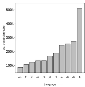
Figure 1.Average vocabulary size for each language.
ing (Dyer, 2007).
Although there is a significant amount of research into improving the treatment of morphology, in this paper we aim to discover the effect that different lev-els of morphology have on translation. We measure the amount of morphological complexity that exists in both languages and then relate this to translation performance.
Some languages seem to be intuitively more com-plex than others, for instance Finnish appears more complex than English. There is, however, no obvi-ous way of measuring this complexity. One method of measuring complexity is by choosing a number of hand-picked, intuitive properties called
complex-ity indicators (Bickel and Nichols, 2005) and then
to count their occurrences. Examples of morpholog-ical complexity indicators could be the number of in-flectional categories or morpheme types in a typical sentence. This method suffers from the major draw-back of finding a principled way of choosing which of the many possible linguistic properties should be included in the list of indicators.
Figure 1 shows the vocabulary size for all rele-vant languages. Each language pair has a slightly different parallel corpus, and so the size of the vo-cabularies for each language needs to be averaged. You can see that the size of the Finnish vocabulary is about six times larger (510,632 words) than the En-glish vocabulary size (88,880 words). The reason for the large vocabulary size is that Finnish is character-ized by a rich inflectional morphology, and it is typo-logically classified as an agglutinative-fusional lan-guage. As a result, words are often polymorphemic, and become remarkably long.
4 Language Relatedness
The morphological complexity of each language in isolation could be misleading. Large differences in morphology between two languages could be more relevant to translation performance than a complex morphology that is very similar in both languages. Languages which are closely related could share morphological forms which might be captured rea-sonably well in translation models. We include a measure of language relatedness in our analyses to take this into account.
Comparative linguistics is a field of linguistics which aims to determine the historical relatedness of languages. Lexicostatistics, developed by Morris Swadesh in the 1950s (Swadesh, 1955), is an ap-proach to comparative linguistics that is appropriate for our purposes because it results in a quantitative measure of relatedness by comparing lists of lexical cognates.
The lexicostatistic percentages are extracted as follows. First, a list of universal culture-free mean-ings are generated. Words are then collected for these meanings for each language under consider-ation. Lists for particular purposes have been gen-erated. For example, we use the data from Dyen et al. (1992) who developed a list of 200 meanings for 84 Indo-European languages. Cognacy decisions are then made by a trained linguist. For each pair of lists the cognacy of a form can be positive, negative or in-determinate. Finally, the lexicostatistic percentage is calculated. This percentage is related to the propor-tion of meanings for a particular language pair that are cognates, i.e. relative to the total without inde-terminacy. Factors such as borrowing, tradition and
Language “animal” “black”
French animal noir
Italian animale nero
Spanish animal negro
English animal black
German tier schwarz
Swedish djur svart
Danish dyr sort
Dutch dier zwart
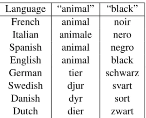
Table 1.An example from the (Dyen et al., 1992) cognate list.
taboo can skew the results.
A portion of the Dyen et al. (1992) data set is shown in Table 1 as an example. From this data a trained linguist would calculate the relatedness of French, Italian and Spanish as 100% because their words for “animal” and “black” are cognates. The Romance languages share one cognate with English, “animal” but not “black”, which means that the lex-icostatistic percentage here would be 50%, and no cognates with the rest of the languages, 0%.
We use the Dyen lexicostatistic percentages as our measure of language relatedness or similarity for all bidirectional language pairs except for Finnish, for which there is not data. Finnish is a Finno-Ugric language and is not part of the Indo-European lan-guage family and is therefore not included in the Dyen results. We were not able to recreate the con-ditions of this study to generate the data for Finnish - expert linguists with knowledge of all the lan-guages would be required. Excluding Finnish would have been a shame as it is an interesting language to look at, however we took care to confirm which effects found in this paper still held when exclud-ing Finnish. Not beexclud-ing part of the Indo-European languages means that its historical similarity with our other languages is very low. For example, En-glish would be more closely related to Hindu than to Finnish. We therefore assume that Finnish has zero similarity with the other languages in the set.
it sv en el pt da es fr nl fi de it
sv en el pt da es fr nl fi de
= 0.17 = 0.35 = 0.52 = 0.7 = 0.87
Figure 2.Language relatedness - the width of the squares indicates the lexicostatical relatedness.
score of 0.87%.
A measure of family relatedness should improve our understanding of the relationship between mor-phological complexity and translation performance.
5 Reordering
Reordering refers to differences in word order that occur in a parallel corpus and the amount of reorder-ing affects the performance of a machine translation system. In order to determine how much it affects performance, we first need to measure it.
5.1 Extracting Reorderings
Reordering is largely driven by syntactic differences between languages and can involve complex rear-rangements between nodes in synchronous trees. Modeling reordering exactly would require a syn-chronous tree-substitution grammar. This represen-tation would be sparse and heterogeneous, limiting its usefulness as a basis for analysis. We make an important simplifying assumption in order for the detection and extraction of reordering data to be tractable and useful. We assume that reordering is a binary process occurring between two blocks that are adjacent in the source. This is similar to the ITG constraint (Wu, 1997), however our reorder-ings are not dependent on a synchronous grammar or a derivation which covers the sentences. There are also similarities with the Human-Targeted
Transla-tion Edit Rate metric (HTER) (Snover et al., 2006) which attempts to find the minimum number of hu-man edits to correct a hypothesis, and admits mov-ing blocks of words, however our algorithm is auto-matic and does not consider inserts or deletes.
Before describing the extraction of reorderings we need to define some concepts. We define ablock A
as consisting of a source span,As, which contains the positions fromAsmintoAsmaxand is aligned to a set of target words. The minimum and maximum positions (Atmin and Atmax) of the aligned target words mark the block’s target span,At.
A reorderingrconsists of the two blocksrAand
rB, which are adjacent in the source and where the relative order of the blocks in the source is reversed in the target. More formally:
rAs < rBs, rAt > rBt, rAsmax =rBsmin−1
A consistent block means that betweenAtminand
Atmax there are no target word positions aligned to source words outside of the block’s source span
As. A reordering is consistent if the block projected fromrAsmintorBsmax is consistent.
The following algorithm detects reorderings and determines the dimensions of the blocks involved. We step through all the source words, and if a word is reordered in the target with respect to the previ-ous source word, then a reordering is said to have occurred. These two words are initially defined as the blocks A and B. Then the algorithm attempts to grow blockAfrom this point towards the source starting position, while the target span ofAis greater than that of blockB, and the new blockAis consis-tent. Finally it attempts to grow blockBtowards the source end position, while the target span of B is less than that ofAand the new reordering is incon-sistent.
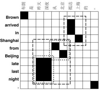
Figure 3.A sentence pair from the test corpus, with its alignment. Two reorderings are shown with two different dash styles.
Battempts to grow the smallest block possible. The reorderings thus extracted would be comparable to those of a right-branching ITG with inversions. This allows for syntactically plausible embedded reorder-ings. This algorithm has the worst case complexity ofO(n22) when the words in the target occur in the reverse order to the words in the source.
5.2 Measuring Reordering
Our reordering extraction technique allows us to an-alyze reorderings in corpora according to the dis-tribution of reordering widths. In order to facilitate the comparison of different corpora, we combine statistics about individual reorderings into a sen-tence level metric which is then averaged over a cor-pus.
RQuantity=
P
r∈R|rAs|+|rBs|
I
whereR is the set of reorderings for a sentence,I
is the source sentence length,AandB are the two blocks involved in the reordering, and |rAs| is the size or span of block A on the source side. RQuan-tity is thus the sum of the spans of all the reordering blocks on the source side, normalized by the length of the source sentence.
RQuantity Europarl, auto align 0.620 WMT06 test, auto align 0.647 WMT06 test, manual align 0.668
Table 2.The reordering quantity for the different reorder-ing corpora for DE-EN.
5.3 Automatic Alignments
Reorderings extracted from manually aligned data can be reliably assumed to be correct. The only exception to this is that embedded reorderings are always right branching and these might contradict syntactic structure. In this paper, however, we use alignments that are automatically extracted from the training corpus using GIZA++. Automatic align-ments could give very different reordering results. In order to justify using reordering data extracted from automatic alignments, we must show that they are similar enough to gold standard alignments to be useful as a measure of reordering.
5.3.1 Experimental Design
We select the German-English language pair be-cause it has a reasonably high level of reordering. A manually aligned German-English corpus was pro-vided by Chris Callison-Burch and consists of the first 220 sentences of test data from the 2006 ACL Workshop on Machine Translation (WMT06) test set. This test set is from a held out portion of the Europarl corpus.
The automatic alignments were extracted by ap-pending the manually aligned sentences on to the respective Europarl v3 corpora and aligning them using GIZA++ (Och and Ney, 2003) and the grow-final-diag algorithm (Koehn et al., 2003).
5.3.2 Results
In order to use automatic alignments to extract re-ordering statistics, we need to show that rere-orderings from automatic alignments are comparable to those from manual alignments.
5 10 15 20
0.0
0.2
0.4
0.6
0.8
1.0
Reordering Width
Av. Reorderings per Sentence
ACL Test Manual ACL Test Automatic Euromatrix
Figure 4. Average number of reorderings per sentence mapped against the total width of the reorderings for DE-EN.
We can see that all three corpora show a similar amount of reordering.
Figure 4 shows that the distribution of reorder-ings between the three corpora is also very similar. These results provide evidence to support our use of automatic reorderings in lieu of manually annotated alignments. Firstly, they show that our WMT06 test corpus is very similar to the Europarl data, which means that any conclusions that we reach using the WMT06 test corpus will be valid for the Europarl data. Secondly, they show that the reordering behav-ior of this corpus is very similar when looking at automatic vs. manual alignments.
Although differences between the reorderings de-tected in the manually and automatically aligned German-English corpora are minor, there we accept that there could be a language pair whose real re-ordering amount is very different to the expected amount given by the automatic alignments. A par-ticular language pair could have alignments that are very unsuited to the stochastic assumptions of the IBM or HMM alignment models. However, manu-ally aligning 110 language pairs is impractical.
5.4 Amount of reordering for the matrix
Extracting the amount of reordering for each of the 110 language pairs in the matrix required a sam-pling approach. We randomly extracted a subset of 2000 sentences from each of the parallel training corpora. From this subset we then extracted the
av-Source Languages
it sv en el pt da es fr nl fi de it
sv en el pt da es fr nl fi de
= 0.13 = 0.25 = 0.38 = 0.51 = 0.64 Target Languages
Figure 5.Reordering amount - the width of the squares indicates the amount of reordering or RQuantity.
erage RQuantity.
In Figure 5 the amount of reordering for each of the language pairs is proportional to the width of the relevant square. Note that the matrix is not quite symmetrical - reordering results differ de-pending on which language is chosen to measure the reordering span. The lowest reordering scores are generally for languages in the same language group (like Portuguese-Spanish, 0.20, and Danish-Swedish, 0.24) and the highest for languages from different groups (like German-French, 0.64, and Finnish-Spanish, 0.61).
5.5 Language similarity and reordering
In this paper we use linear regression models to de-termine the correlation and significance of various explanatory variables with the dependent variable, the BLEU score. Ideally the explanatory variables involved should be independent of each other, how-ever the amount of reordering in a parallel corpus could easily be influenced by family relatedness. We investigate the correlation between these variables.
●●
● ●
●●● ●
●●● ●
●
●
● ●
● ●
● ●
●
●
●● ●
● ●
● ●
● ●
●
● ●
● ● ●
● ● ●
● ●
● ●
● ● ●
● ● ●
● ● ●
● ●
●●
●
● ● ●
●
●●● ●
● ● ●●
●
● ● ●
● ●
● ●
● ● ●●●● ●
●
● ●
●●● ● ●●●● ●
● ●
●●●●●● ●●
0.2 0.3 0.4 0.5 0.6
0.0
0.2
0.4
0.6
0.8
Reordering Amount
Language Similarity
Figure 6. Reordering compared to language similarity with regression.
6 Experimental Design
We used the phrase-based model Moses (Koehn et al., 2007) for the experiments with all the standard settings, including a lexicalized reordering model, and a 5-gram language model. Tests were run on the ACL WSMT 2008 test set (Callison-Burch et al., 2008).
6.1 Evaluation of Translation Performance
We use the BLEU score (Papineni et al., 2002) to evaluate our systems. While the role of BLEU in
machine translation evaluation is a much discussed topic, it is generally assumed to be a adequate metric for comparing systems of the same type.
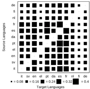
Figure 7 shows the BLEUscore results for the
ma-trix. Comparing this figure to Figure 5 there seems to be a clear negative correlation between reordering amount and translation performance.
6.2 Regression Analysis
We perform multiple linear regression analyses us-ing measures of morphological complexity, lan-guage relatedness and reordering amount as our in-dependent variables. The in-dependent variable is the translation performance metric, the BLEUscore.
We then use a t-test to determine whether the co-efficients for the independent variables are reliably different from zero. We also test how well the model explains the data using an R2 test. The two-tailed significance levels of coefficients and R2 are also
Source Languages
it sv en el pt da es fr nl fi de it
sv en el pt da es fr nl fi de
= 0.08 = 0.16 = 0.24 = 0.32 = 0.4 Target Languages
Figure 7.System performance - the width of the squares indicates the system performance in terms of the BLEU
score.
Explanatory Variable Coefficient
Target Vocab. Size -3.885 ***
Language Similarity 3.274 ***
Reordering Amount -1.883 ***
Target Vocab. Size2 1.017 ***
Language Similarity2 -1.858 ** Interaction: Reord/Sim -1.4536 ***
Table 3.The impact of the various explanatory features on the BLEUscore via their coefficients in the minimal ad-equate model.
given where * means p<0.05, ** means p<0.01, and *** means p<0.001.
7 Results
7.1 Combined Model
The first question we are interested in answering is which factors contribute most and how they interact. We fit a multiple regression model to the data. The source vocabulary size has no significant effect on the outcome. All explanatory variable vectors were normalized to be more comparable.
variation in BLEU can be explained by these three factors. The interaction of reordering amount and language relatedness is the product of the values of these two features, and in itself it is an important ex-planatory feature.
To make sure that our regression is valid, we need to consider the special case of Finnish. Data points where Finnish is the target language are outliers. Finnish has the lowest language similarity with all other languages, and the largest vocabulary size. It also has very high amounts of reordering, and the lowest BLEUscores when it is the target language. The multiple regression of Table 3 where Finnish as the source and target language is excluded, shows that all the effects are still very significant, with the model’sR2 dropping only slightly to 0.68.
The coefficients of the variables in the multiple regression model have only limited usefulness as a measure of the impact of the explanatory variables in the model. One important factor to consider is that if the explanatory variables are highly correlated, then the values of the coefficients are unstable. The model could attribute more importance to one or the other variable without changing the overall fit of the model. This is the problem of multicollinearity. Our explanatory variables are all correlated, but a large amount of this correlation can be explained by look-ing at language pairs with Finnish as the target lan-guage. Excluding these data points, only language relatedness and reordering amount are still corre-lated, see Section 5.5 for more details.
7.2 Contribution in isolation
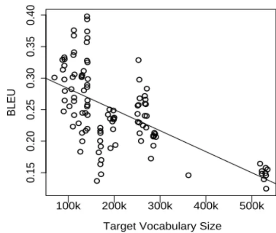
In order to establish the relative contribution of vari-ables, we isolate their impact on the BLEUscore by modeling them in separate linear regression models. Figure 8 shows a simple regression model over the plot of BLEU scores against target vocabulary size. This figure shows groups of data points with the same target language in almost vertical lines. Each language pair has a separate parallel training corpus, but the target vocabulary size for one language will be very similar in all of them. The variance in BLEU
amongst the group with the same target language is then largely explained by the other factors, similarity and reordering.
Figure 9 shows a simple regression model over the plot of BLEUscores against source vocabulary size.
● ●
● ●
● ●
● ● ●
● ●
● ●
● ● ●
● ●
● ●
● ●
●
● ●
● ● ● ●
● ● ●
● ●
● ●
● ●
●
● ● ●
● ● ● ● ●
● ●
● ●
●
●
● ●
●● ● ● ● ●
● ● ●
●● ●
● ●
● ● ●● ● ● ●
● ● ● ●
● ●
●
● ●
●
● ●
● ●●● ● ●● ● ●
● ●
● ●
● ●
●
● ● ●
0.15
0.20
0.25
0.30
0.35
0.40
Target Vocabulary Size
BLEU
| | | | | 100k 200k 300k 400k 500k
Figure 8.BLEUscore of experiments compared to target vocabulary size showing regression
This regression model shows that in isolation source vocabulary size is significant (p<0.05), but that this is due to the distorting effect of Finnish. Excluding results that include Finnish, there is no longer any significant correlation with BLEU. The source mor-phology might be significant for models trained on smaller data sets, where model parameters are more sensitive to sparse counts.
Figure 10 shows the simple regression model over the plot of BLEU scores against the amount of re-ordering. This graph shows that with more reorder-ing, the performance of the translation model re-duces. Data points with low levels of reordering and high BLEU scores tend to be language pairs where both languages are Romance languages. High BLEU
scores with high levels of reordering tend to have German as the source language and a Romance lan-guage as the target.
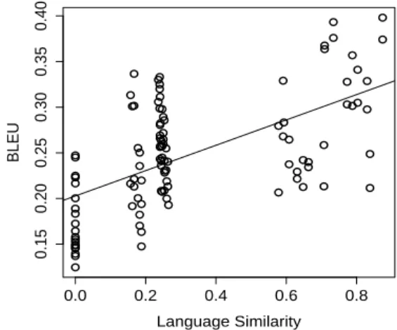
Figure 11 shows the simple regression model over the plot of BLEU scores against the amount of lan-guage relatedness. The left hand line of points are the results involving Finnish. The vertical group of points just to the right, are results where Greek is involved. The next set of points are the results where the translation is between Germanic and Ro-mance languages. The final cloud to the right are re-sults where languages are in the same family, either within the Romance or the Germanic languages.
● ● ● ● ● ● ● ● ● ● ● ● ● ● ● ● ● ● ● ● ● ● ● ● ● ● ● ● ● ● ● ● ● ● ● ● ● ● ● ● ● ● ● ● ● ● ● ● ● ● ● ● ● ● ● ● ● ● ● ● ● ● ● ● ● ● ● ●● ● ● ● ● ● ● ● ● ● ●● ● ● ● ●● ● ● ● ●● ● ● ●● ● ● ● ● ● ● ● ● ● ● ● ● ● 0.15 0.20 0.25 0.30 0.35 0.40
Source Vocabulary Size
BLEU
| | | | | 100k 200k 300k 400k 500k
● ● ● ● ● ● ●● ● ● ● ● Finnish Other
Figure 9.BLEUscore of experiments compared to source vocabulary size highlighting the Finnish source vocabu-lary data points. The regression includes Finnish in the model.
Explanatory Variable R2 Target Vocab. Size 0.388 *** Reordering Amount 0.384 *** Language Similarity 0.366 *** Source Vocab. Size 0.045 * Excluding Finnish
Target Vocab. Size 0.219 *** Reordering Amount 0.332 *** Language Similarity 0.188 *** Source Vocab. Size 0.007
Table 4.Goodness of fit of different simple linear regres-sion models which use just one explanatory variable. The significance level represents the level of probability that the regression is appropriate. The second set of results excludes Finnish in the source and target language.
are simple regression models, with just one explana-tory variable, multicolinearity is avoided. This table shows that each of the main effects explains about a third of the variance of BLEU, which means that they can be considered to be of equal importance. When Finnish examples are removed, only reordering re-tains its power, and target vocabulary and language similarity reduce in importance and source vocabu-lary size no longer correlates with performance.
8 Conclusion
We have broken down the relative impact of the characteristics of different language pairs on
trans-● ● ● ● ● ● ● ● ● ● ● ● ● ● ● ● ● ● ● ● ● ● ● ● ● ● ● ● ● ● ● ● ● ● ● ● ● ● ● ● ● ● ● ● ● ● ● ● ● ● ● ● ● ● ● ●● ● ● ● ● ● ● ● ● ● ● ● ● ● ● ● ● ● ● ● ● ● ● ● ● ● ● ● ● ● ● ● ● ● ●● ● ● ●● ● ● ● ● ● ● ● ● ● ● ●
0.2 0.3 0.4 0.5 0.6
0.15 0.20 0.25 0.30 0.35 0.40 Reordering Amount BLEU
Figure 10. BLEU score of experiments compared to amount of reordering.
● ● ● ● ● ● ● ● ● ● ● ● ● ● ● ● ● ● ● ● ● ● ● ● ● ●● ● ● ● ● ● ● ● ● ● ● ● ● ● ● ● ● ● ● ● ● ● ● ● ● ● ● ● ● ● ● ● ● ● ● ● ● ● ● ● ● ● ● ● ● ● ● ● ● ● ● ● ● ● ● ● ● ● ● ● ● ● ● ● ● ● ● ● ● ● ● ● ● ● ● ● ● ● ● ● ●
0.0 0.2 0.4 0.6 0.8
0.15 0.20 0.25 0.30 0.35 0.40 Language Similarity BLEU
Figure 11.BLEUscore of experiments compared to lan-guage relatedness.
lation performance. The analysis done is able to ac-count for a large percentage (75%) of the variabil-ity of the performance of the system, which shows that we have captured the core challenges for the phrase-based model. We have shown that their im-pact is about the same, with reordering and target vocabulary size each contributing about 0.38%.
References
Balthasar Bickel and Johanna Nichols, 2005. The World Atlas of Language Structures, chapter Inflectional syn-thesis of the verb. Oxford University Press.
Peter F. Brown, Stephen A. Della Pietra, Vincent J. Della Pietra, and Robert L. Mercer. 1993. The mathematics of machine translation: Parameter estimation. Compu-tational Linguistics, 19(2):263–311.
Chris Callison-Burch, Cameron Fordyce, Philipp Koehn, Christof Monz, and Josh Schroeder. 2008. Further meta-evaluation of machine translation. In Proceed-ings of the Third Workshop on Statistical Machine Translation, pages 70–106, Columbus, Ohio, June. As-sociation for Computational Linguistics.
Isidore Dyen, Joseph Kruskal, and Paul Black. 1992. An indoeuropean classification, a lexicostatistical experi-ment.Transactions of the American Philosophical So-ciety, 82(5).
Chris Dyer. 2007. The ’noisier channel’: Transla-tion from morphologically complex languages. In Proceedings on the Workshop on Statistical Machine Translation, Prague, Czech Republic.
Sharon Goldwater and David McClosky. 2005. Im-proving statistical MT through morphological analy-sis. InProceedings of Empirical Methods in Natural Language Processing.
Philipp Koehn, Franz Och, and Daniel Marcu. 2003. Sta-tistical phrase-based translation. InProceedings of the Human Language Technology and North American As-sociation for Computational Linguistics Conference, pages 127–133, Edmonton, Canada. Association for Computational Linguistics.
Philipp Koehn, Hieu Hoang, Alexandra Birch, Chris Callison-Burch, Marcello Federico, Nicola Bertoldi, Brooke Cowan, Wade Shen, Christine Moran, Richard Zens, Chris Dyer, Ondrej Bojar, Alexandra Constantin, and Evan Herbst. 2007. Moses: Open source toolkit for statistical machine translation. In Proceedings of the Association for Computational Linguistics Com-panion Demo and Poster Sessions, pages 177–180, Prague, Czech Republic. Association for Computa-tional Linguistics.
Philipp Koehn. 2005. Europarl: A parallel corpus for statistical machine translation. InProceedings of MT-Summit.
Franz Josef Och and Hermann Ney. 2003. A system-atic comparison of various statistical alignment mod-els. Computational Linguistics, 29(1):9–51.
Kishore Papineni, Salim Roukos, Todd Ward, and Wei-Jing Zhu. 2002. BLEU: a method for automatic evalu-ation of machine translevalu-ation. InProceedings of the As-sociation for Computational Linguistics, pages 311– 318, Philadelphia, USA.
M Snover, B Dorr, R Schwartz, L Micciulla, and J Makhoul. 2006. A study of translation edit rate with targeted human annotation. InAMTA.
Morris Swadesh. 1955. Lexicostatistic dating of prehis-toric ethnic contacts. InProceedings American Philo-sophical Society, volume 96, pages 452–463.
David Talbot and Miles Osborne. 2006. Modelling lex-ical redundancy for machine translation. In Proceed-ings of the Association of Computational Linguistics, Sydney, Australia.