p93 総合研究大学院大学学術情報リポジトリ p93

Particle Accelerators,1993,Vol.41,pp93-115

Reprints available directly from the publisher Photocopying permitted by license only

©1993Gordon&Breach Science Publishers, S.A. Printed in the United States of America.

ONE-DIMENSIONAL

RIGID GAUSSIAN MODEL

OF THE BEAM-BEAM INTERACTION

KOHlI HIRATA

KEK, National Laboratory for High Energy Physics, Tsukuba, Ibaraki 305, Japan

(Received31 July 1992; in final form 24 December 1992)

A simple one-dimensional model of the beam-beam interaction (sheet-sheet interaction) and its rigid-Gaussian approximation for the coherent barycentre motion are studied in order to examine the usefulness of the rigid- Gaussian approximation. Effects of primordial separation between beams are studied in detail. The spontaneous beam separation for the integer resonance can be embedded in a cusp catastrophe structure as a special case. A new technique is introduced to the calculation of the beam-beam force for the multiparticle tracking, without relying on the Gaussian approximation. The rigid-Gaussian approximation is shown to be reliable enough for evaluating closed-orbit effects, except for some extremely exceptional cases.

KEY WORDS: Beam-beam interaction, Rigid-Gaussian model

INTRODUCTION

When two beams collide in a storage ring, they affect each other through the beam-beam force. 1 This effect has been studied for many years. Among many approaches, the so- called coherent approach²,3, forms one of the dominant streams. Particularly important issue there is the coherent barycentre motions, where the most natural tool is the rigid Gaussian model4 (RGM): the distribution function is assumed to be a Gaussian with fixed variances. It gave fairly accurate estimate of the beam-beam modes,5,6,7 unexpected instability structure of the two-ring colliders with different circumferences⁸ and many other practically useful predictions.9,10,1l In these cases, since beams are supposed to collide head-on, the analysis. could be concentrated on the linear stability of the nominal or unperturbed closed orbit, using the linear approximation of the beam-beam force. (A violation of the linear stability causes the spontaneous beam separation (8B8).4) For more general cases, we should note that the use of the linearized treatment is not justified, at least automatically.

At present, many future projects, such as Band¢factories,12,13,14,15,16,17 are employing two-ring scheme. In two-ring colliders, it seems difficult to make bunches collide always exactly head-on. When the collision has an offset, i.e., primordial beam separation, the linear analysis of the beam-beam force at the nominal orbit is no longer reliable in evaluating the instability threshold. The beam-beam kick depends on the offset but the offset is affected by the beam-beam force. Also, many projects are ready to have

93

94 K. HIRATA

many bunches in each beam. We thus should study not only the collision at the central collision point but also at the peripheral collision points. 18,19,20 Through the latter effect, all bunches are coupled.

To study these problems, with the limited ability of the present-day computers, the nonlinear RGM seems to be the unique tool. The multiparticle tracking, though more reliable, seems impossible from computation time point of view. The RGM is tractable. The question is whether it is reliable or not. In other words, we should find to what extent it is reliable. Some of immediate shortcomings are;

1. Fundamental assumption is that the whole bunch keeps its union. If it is split into some clusters, the failure of RGM is evident.

2. The possible modification of beam sizes are overlooked. This may affect the linear part of the force and the threshold of linear instabilities. The beam size effect itself is overlooked also: the RGM may predict that the whole bunch is caught by a nonlinear resonance, even if the resonance is too small to keep the whole bunch.

3. We should ignore the coupling between higher order modes: there is no hope to include the tune shift factor,21,22 for example.

In this paper, in order to study the reliability of RGM, we examine a simplified beam-beam interaction, where the multiparticle tracking can be performed relatively easy without recourse to the Gaussian approximation in calculating the beam-beam force. This is an abstraction from, but not identical with, the vertical interaction of very flat beams. We study this simplified interaction and apply the rigid-Gaussian approximation to this case. This is simple enough to permit us some analytical investigations but not too simple to lose the physical significance. Since the main target of the (nonlinear) rigid-Gaussian approximation is the closed orbit effect, we study it in detail (some partial results have already been published elsewhere,19,23,24) and will examine some calculation techniques used within the RGM scheme. We will compare the Gaussian approximation with more reliable multiparticle tracking results for some cases. For simplicity, we assume only one interaction point (IP) and one bunch in each beam. More general cases, however, can be studied by a straightforward extension.

In the next section, we define the one-dimensional RGM, called RGM1. Then in section 3, we study its behaviours in terms of the closed orbits formation in the presence of primordial offset. A comparison with the multiparticle tracking will be done in section 4. Section 5 will be devoted to discussion, summary and conclusion.

2 RGM1: ONE-DIMENSIONAL RIGID GUASSINA MODEL

In RGM, we are interested in the barycentre variables z± ｾ (z)± only and ignore the possible effects of the beam-beam interaction on beam sizes or beam distributions. Here z stands for either horizontal(x)or vertical(y)coordinates and ( )± refers to the average over the e±bunch. The rms beam sizes are

In RGM, however, the effective beam sizes

are more relevant. In this connection, we introduce the coherent beam-beam parameter

(1)

(2) Note the difference from the incoherent beam-beam ｰ｡ｲ｡ｭ･ｴ･ｲｾＮ When two colliding bunches have the same rms beam sizes, we have *

:=:

⁼⁼ｾＯＲＮ

Let us assume that the beams are quite flat

and consider the vertical motion only. That is, we assume the horizontal beam-beam effect weak enough. If we assume that

x±

⁼⁼ 0 and that

y <<

ｾｸＬ we can get, as the beam-beam kick,

8-¹ _ N=r-r^e y!2; f

_{(Y+ -} y-

+ Do) Y± - =f l'± ｾｸ er ｨｾｹ

.

HereN± is the number of particles in e± bunch,

r

the relativistic Lorentz factor and Dothe nominal (i.e. without beam-beam effect) difference between closed orbits of both beams at the IP. We call Do the primordial beam separation. This model is called the one-dimensional rigid Gaussian model (RGM1). If the separationy+ - y-+Do becomes so large that it is comparable to ｾｸＬ the force should begin to decrease. Such a case is not considered here. The corresponding incoherent force will be discussed in Sect.5.

We parametrize variables as

j3^{±- I}

P -

^y y±

± - E '

y

where j3y is the nominal vertical betatron function at the IP. In these variables, the dynamics is as follows:

At the IP, (Beam-Beam Kick) we have

where

F(x)

=

(27r)3/2erf (

_ｾＩ

.

(3)

(4)

* Note that we include the effectofthe beam sizesonthe beam-beam interaction⁵but not vice versa. In RGM, the fundamental assumption is that bunches move rigidly with their Gaussian distribution kept fixed. A direct consequence is that the transverse kick for the barycenter is different from a kick for a particle situating at the place of the barycenter.

96

During the arc , we have

where V± is defined by

K. HIRATA

(5)

V±

== ( _{ｃｏｾｊＭｌﾱ}

- slnJ-L±

sinJ-L± ) . cosJ-L±

Here J-L

==

21rv and A±

==

exp( -1/T±): T± being the vertical damping time measured by the revolution time. These two mappings are applied in alternation. Since A± is usually very close to unity, this will be omitted in expressing the closed orbits. The caseｾ

==

0 was studied in Ref.^4.

3 CLOSED ORDBIS IN RGMI The vector

_ A A A A t

W

==

(Y+,P+, Y_,P_)

is expected to fall into an equilibrium eventually due to the radiation damping, as long as it starts already close to the equilibrium value. This is the closed orbit, which we are interested in here. Exceptions arise in the following cases:

1. When the closed orbit is unstable. This corresponds to the linear instabilities.⁴ Ac- cording to Ref.4, we classify cases with ｾ

==

0 as follows:

half-integer resonance It occurs when v+,:S1/2+integer or v_,:S1/2+integer. When it occurs, the system falls into the period-two closed orbit, that is, the orbit at the IP takes two values alternatively every tum with finite separation between beams. sum resonance It occurs whenv++v_,:Sinteger. When it occurs, the steady state is

a limit cycle and the behaviour is multi-periodic. (This can be read from Fig. 3.1). integer resonance It occurs whenv+,:Sinteger orv_,:Sinteger. When it occurs, the system can have two different closed orbits: one of them is chosen spontaneously. All of these are spontaneous breaking of the symmetry and give sudden changes. 2. Or, when the stability region inW space is too small. This corresponds to nonlinear

resonances, close to the closed orbit. W is attracted to one of them.

We will mainly discuss the linear resonance of the closed orbit with ｾ

i=

0 and discuss the latter a little in section 4.4.

3.1 Real Separation and Betatron Amplitudes

The closed orbit at the IP_ (i.e. just before the beam-beam kick), if it exists, is the solution of

W

==

V(W+F),

ONE-DIMENSIONAL RIGID GAUSSIAN MODEL

F-==

The solution is expressed as

It gives

o

-3+F(Y+ - Y- ＫｾＩ

o

+3_F(Y+ - Y- _ＫｾＩ

W

=

1

_ｾ

VF.

1 ｾ M± ^{A A}

=fT'::±cot - 2 -F (Y+ - Y- +_ｾＩＬ

1 ^{A A}

±T

3 ±F(Y+ - Y- +_ｾＩＮ

(6)

Thus, the real beam separation (in unit of_ｾｹＩＬ

S

-== Y+ -

_Y-

_ＫｾＬ is determined by the following consistency equation

(7)

where

G(Y) -== - - - --2Y

ｾ M+ ｾ M-

.::+cot - 2 - + .::- cot - 2 - The solution is illustrated in Fig. 1.

From Eq. (7) and Fig.l, it can be observed that, as long as the closed orbit exists,

ｾ ｾ M+ ｾ M- >0

lor .::+cot - 2 -+ .::-cot - 2 -< . In case where 3+ -== 3_,this condition is equivalent to t

(8)

A numerical example of the solution of Eq. (7) can be obtained easily. Here, instead, we track W starting from a point nearby the solution and apply Eq. (3) and Eq. (5) alternately in order to check the stability of the solution altogether. The results are shown in Fig.3.!, where

S

is given as a function ofv+ but with v_ being fixed. We track Wand plot

S

for last 20 turns. From the figure, we see three exceptional peaks, which correspond to the half integerＨｶＫｾＰＮＵＩＬ the sum(v+;S0.8)and the integerＨｶＫｾｉＩ

resonances. Otherwise, the solution is identical with that of Eq. (7). We will discuss them in section 3.2. The symbol ｾ indicates that the instability occurs just below the resonant tune.

t In the present context, the integer part of the tune is irrelevant so that, for example, this equation should be understood as[v++v_] _>0 for the upper case and< 1 for the lower case, where [ ] is the noninteger part.

G

---+---

_F-

y - y

+ -

FIGURE 1: The real separationS(indicated by a solid arrow) at the IP. The nominal one_ＨｾＩ is shown by the dotted arrow. The curve is the functionF, Eq. (4), and the 0 indicates the solution of Eq. (7). Similar graph for a different set of parameters can be found in Fig. 3.2.

Ｎｾ

o

20

o

1---:::::.. ----til.:<}-/

..^ｾＮ

-1 -20

0.8

0.4 0.6

v+ 0.2

- 40 ...-'--'---'--'-...L..-J.----L..-J...-'--'---'--'-...L..-J.-'--L...L.-..I....-l--'---'---'--'

o

0.8

0.4 0.6

v+ 0.2

_2l..-...1..-...l....-L----'--J--1--..L.-..I.---'---'---'--.L...l..-...l....-L----'--JL...L..-...L...-L...L...-L--'--.I...-I

o

FIGURE 2: Thev+dependence of the separationSat the IP. Parameters arev_ = 0.2, T ±= 500, B±= 0.03 andｾ = 1. Both graphs are results of tracking and are identical except for the vertical scales.

ONE-DIMENSIONAL RIGID GAUSSIAN MODEL 99

0.6

0.4

0.2

0.0

o

^{0.02 0.04 0.06 0.08} 0.1 -

FIGURE 3: The 3 dependence of the luminosity reduction factorR(S). (3+ = 3_ is assumed). Tunes (v+ =v -)are written on the corresponding lines. Parameters are T± =500 andｾ =1.

The separation

S

perturbs the luminosity. In this connection, it is convenient to introduce the luminosity reduction factorR by

(9)

Here ( )av is the average over many turns. In the presence of the separation

S,

the luminosityL is reduced as

L(S) = L(O)R(S).

The beam-beam force depends on the real separation at the IP. The real separation, on the other hand, depends on the beam-beam force. InFig. 3.1, we show R as a function of3. The decrease (v < 0.5) and increase (v >0.5) of the separation

S

for increasing 3 are clearly seen. For v < 0.5, the separation increases suddenly at some value of 3. This increase corresponds to a peak in Fig. 3.1. For v > 0.5, however, no sudden change is observed: the separation increases monotonically as 3 increases.

Let us tum to the closed orbit amplitude in the arc

A±.

The closed orbits in the arc, or its amplitude, depends also on the beam-beam force. From Eqs.(6) and (7), we obtain the betatron amplitude in the arc,

A

_V

A2 A2 _.::.±

I " " I

A±

=

Y±+P±

=

ｆＨｙＫＭｙ｟ＫｾＩ .

21

sin f.t 2^{± I}

(10)

Here the argument of F is the solution of Eq. (7). We show

A

as a function of tune (similar to Fig. 3.1) in Fig. 3.1.

The instability structure is the same as the case of the separation

S.

A graph (similar to Fig. 3.1) of

A

as a function of 3 is shown in Fig. 3.1.

-+ 2.0 A

1.5

1.0

0.5

0.0 _V+

0 0.2 0.4 0.6 0.8 1

FIGURE 4: The1/+dependence ofIi+. Parameters are1/_ ₌0.2, T ± =500, 3± =0.03 andｾ = 1.

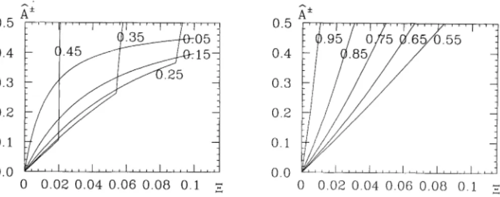
0.5 A:± 0.5 A:±

.05

0.4 .15 0.4

0.3 0.3

0.2 0.2

0.1 0.1

0.0 0.0

0 0.02 0.04 0.06 0.08 0.1 ... 0 0.02 0.04 0.06 0.08 0.1 ...

FIGURE 5: The 3 dependence of the amplitude in the arcIi . Parameters are the same as those used in Fig. 3.1.

Contrary to the case of the real separation,

S,

the amplitude

A

increases monotonically as 3 increases. There exists a sudden increase of

A

at a certain value of 3 whenever v < 0.5. For the reasonable value of3 and v,F in Eq. (10) does not largely depend on 3, we can say that

A±

is almost proportional to3±.

Thus, we have seen that the real separation

S

and the betatron amplitudes

A

are the solutions of Eqs.(7) and (10), respectively except in the cases of resonances. The separation

S

affects the luminosity directly. The betatron amplitude

_A

in the arc may also have serious effects: the emittance, chromaticity etc may change according to the current, in addition to the lifetime and background issues. From Figs.3.1 and 3.1, we can make the following comment: if the nominal separation at the IP is unavoidable, v+ should be chosen around 0.2 to 0.3, because the reduction of the luminosity can be improved and the closed orbits in the arc is suppressed. This, of course, applies to the case with v_ == 0.2. A consideration on nonlinear resonances is also needed. The important thing here, however, is that the luminosity reduction is not the only criterion in choosing the tunes.

(a)

ONE-DIMENSIONAL RIGID GAUSSIAN MODEL

(b)

p+-p-

10

a / ^G

₅

·F

y - y ₀

+ -

C

-5

-10

...

FIGURE 6: Nontrivial period-one fixed points near the integer resonance, where the closed orbit solution is not unique. (a) Three solutions of Eq. (7). Two of them a and c are stable. (b) The corresponding phase space (without damping) of(1\ - y- ,p^{+ -} P-) with several different initial conditions and withT = 00. _Two

elliptic fixed points (centers of circles) correspond to a and c in (a) and the hyperbolic fixed point to b.

3.2 Catastrophe Structure of Instability

Here we discuss the exceptional cases, represented by the three peaks in Figs. 3.1 and 3.1. These cases occur when the solution of Eq. (7) is either unstable or bi-stable. The peaks seem to correspond to half-integer, sum and integer resonances, which were found⁴ by a linear analysis withｾ

== o.

The qualitative behaviour of beams at the half-integer and the sum resonances seem to be identical between cases ofｾ

==

0 and ｾ

i

O. In these two cases, the solution of Eq. (6) exists uniquely but becomes unstable when the resonance condition is satisfied.

In the integer resonance case, there is a qualitative difference. The situation changes drastically. As clear from Fig. 3.1, there is no sudden change of the separation but it increases gradually. Seemingly, this is nothing but the COD behaviour under a dipole perturbation. Where has the SBS (Spontaneous Beam Separation) gone? In this case, contrary to the other cases, it can be shown that the solution of Eq. (6) is stable but not unique. See Fig. 3.2.

In the left figure, the pointa corresponds to the line in Fig.3.I. There are two other intersections, band c. It can be shown that b is unstable, while c is stable. In the right figure, a Poincare surface plot is shown for the case corresponding to the left figure. Two clusters of circles are seen, the centres of which correspond to a and c. Thus there are two stable period-one closed orbits. The system chooses one of them according to the initial conditions.

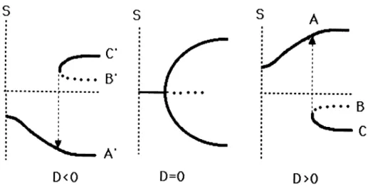
The stability situation is illustrated in Fig.3.2. For the integer resonance case, the total structure is that of the cusp catastrophe,25 where ｾ

==

0 is the special case. Imagine the

s _{s s A}

I I I I I I I I I

. ...•...I I

ｌｾ

r

I.

I • • • • •

I

•...I,.••..••..

0<0 0=0 _0>0

FIGURE 7: A schematic stability diagram for the case where v is a little smaller than an integer. The dotted lines correspond to the unstable solution. The horizontal axis is either v or 3 and the vertical S .The arrow shows the jump when the system is moving from right to left (3 or v are decreasing). ForD #-0, the lines extending to 3 =

_°

(A and A') are called the natural branches and the others (C and C') the unnatural branches.

system is on the line C in Fig. 3.2 and

:=:

orv decreases. When the system reaches at the edge, it should jump into the other branch. This jump is illustrated in the figure. After that, if ｾ changes its sign, artificially or accidentally, the system should jump again to the original branch. Thus, with ｾ and

:=:

or v, we can play with this type of sudden jumps with hysteresis. The lines represented by A or A' are called the natural branches and the other, C or C', the unnatural branches. In Figs. 3.1 and 3.1, only the natural branch appears because we started tracking near it.

This structure can be seen also in a multiparticle tracking, see section 4.2

4 THE MULTIPARTICLE TRACKING Here, we discuss the reliability of the RGM.

Instead of Eq. (2), which deals with the coherent kick, we study an incoherent force (11) where

(JjG

is the nominal beam size andTJis the nominal incoherent beam-beam param- eter:

(12) and

E(y) = {

_ｾＱ

_y^y>O

_<

_{0 .} ⁽¹³⁾

Here p is the vertical distribution of particles and is not assumed to be a Gaussian. Thanks to the one-dimensional nature of the force, in the multiparticle tracking, there is no need to rely on the Gaussian approximation to calculate the beam-beam kick. To obtain the kick applied to an e+ particle, we count the number ofe - particles which are above that e+ particle. This is applicable to any distribution. The importance to calculate the force without relying on Gaussian approximation was stressed by many authors. For round-beam, though one-dimensional, or for more general two- and three- dimensional distributions, the calculation is much more complicated and needs more careful treatments.26,27

This model is the incoherent version of the RGMI, studied in previous sections. We have integrated over the horizontal direction assuming that the horizontal distributions are Gaussian. Thus the kick Eq. (11) can be called sheet-sheet force+. The process during the arc is according to the symmetric radiation.²⁸The basis of the RGMI, Eq. (2), is obtained from Eq. (11) by the averaging

assuming that both ofp+ andp_ are Gaussians. Thus the RGM is doubly based on the Gaussian approximation.

4.1 Union of a Bunch

The largest possible shortcoming of the RGM may be that it should be erroneous if a single bunch is split into two or more clusters in the phase space. The first necessary condition of using the RGM is that the whole bunch should keep its union. In fact, it is quite easy, in the multiparticle tracking, to get an equilibrium distribution where one beam is split into two clusters. See Fig. 4.1, where the phase spaces of e+ and e-

bunches are shown separately. Here we use

The figure corresponds to the case where Do

==

0 and to the weak-strong situation, that is when 3+

«

3_ or 3+

»

3_.

The result shown in Fig. 4.1 is quite natural. In the weak-strong situation, the strong beam is not affected at all. Correspondingly, the particles in the weak-beam are little correlated to each other. Thus, whenever there are several stable fixed points, each particle chooses one of them depending only on the initial conditions. The equilibrium

:I: To avoid misunderstanding, some comments seem useful; Because of the averaging over horizontal di- rection, the incoherent tune shift for a particle (sheet) is notrJbut 8v ｾ rJ /-12. Ifthe bunch is a Gaussian, Eq. (11) is reduced to

P

10

5 ⁵

o o

-5 -5

5

10

y o

-5

- 10 ｌＮＮＭＮＮｌＮＮＮＮＭＮＮｬＭＭｊＮＮＮＭＮＮＮＮｬＭＮＮＮＮｌＮＮＮＮＭＮＮＮＮＮＧＭＭＭＭｊＮＮＮＭＮｌＮＮＭＭｌＮＮＮＭＮＮｌＮＭＮＮＮＮｌＭＮｌＭＮＮＮＭＮＮｌＮＭＮＮｌＮＮＭＭｌＮＭＭｌＮＮＮＭＮＮｌＮＭｾ - ₁₀ L-.L.--L.--'---'--...---J....-...L---'---'--..l...I..---'----I-...L..--&--...

-10 -5 0 5 10 -10

y+

FIGURE 8: A multiparticle tracking result. The equilibrium phase space distribution for (3+,3_)=(0.055,0.005), v± ₌0.95,TE=^{100 and Do}=^O. Left:(Y+,P+). Right:(Y-,P_).

P

10

5

5

o o

-5 -5

5 10

y o

-5

- 10 L...-...L-..I..----I...J...L...I..---I...L....-...L...L..--J...-....l-..L.-J - ₁₀ L.--L..-...L.---L...L...ＭＭＭｌＭＭｉＭＭＭＭＧＭＭＭＧＭＭＮＮｌＮＮＮＭＮＮＮｌＭＭＭｌＭＭＭｉＮＮＭＮｌＭｾＮｌＮＮＭＮＮｊ

-10 -5 0 5 10 -10

y+

FIGURE 9: A multiparticle tracking result. The equilibrium phase space distribution for (3+, 3_) (0.03,0.03), v± =0.95,TE=100 and Do=O. Left:(Y+,P+). Right:(Y_,P _).

distribution seems unique: between stable fixed points, the transition probabilities from one to another should balance.

In the strong-strong situation, that is, when 3+ｾ 3_, we have a different picture. See Fig. 4.1. Each bunch is concentrated in its phase space. If we increase 3_ from the state such as that in Fig. 4.1, the system changes to that in Fig. 4.1 at certain point. We thus may conclude that in the strong-strong situation, i.e. when 3+ ｾ 3_, the bunches behave in the coherent manner and the unity of the bunch is kept§, as Fig. 4.1, so that the RGM should work well. Finally, note that when a bunch is split into clusters, the usual technique of the multiparticle tracking, i.e., calculating rms beam sizes and evaluating the beam-beam force using them, cannot be applied.

4.2 Catastrophe

Let us examine the catastrophe structure considered in section 3.2. In Fig. 4.2, we compare the multiparticle tracking results with the prediction of RGM 1 for ｾ == 1 (Do == ｾｹＩＮ The figure shows that the agreement is excellent. The small disagreement may come from the change of the beam sizes in the multiparticle tracking and a possible deviation from the Gaussian distribution, which are ignored in RGMI. (In the figure, we showed the simulation estimates of realｾ as error bars. Any significant deviations ofｾ

from its nominal value was not observed.

One remarkable thing is that the transition from the unnatural branch to the natural branch occurs at a little larger value of 3. The reason is clear. As can be seen from Fig. 3.2, the stable region of the unnatural branch in the phase space, (the left circle in the right figure of Fig. 3.2), is quite small for the parameters close to the critical value. If the stable region is too small, it cannot hold the bunch.

4.3 Beam Size Increase

Another possible source of shortcomings is that the beam size can change before reaching the dipole instability threshold. This can enhance ｾ so that reduce 3. If this effect is too strong, it is possible that the dipole instability cannot happen. This problem was already discussed in Ref. 4

§ For the completeness of the statement, we should add more. In the multiparticle tracking, for unrealistically large value of 3, it is possible to get a state like Fig. 4.1 for the case with 3+ = 3_. An example is as follows. From the parameters used in Fig. 4.1, we increase 3_ gradually. When it reaches 0.06, we see that thee+bunch is still split. It is so even when 3- is increased a little more. Thus, for 3+=3_ =0.06, four different states are stable:

1. e+is split ande - is concentrated. 2. e+ is concentrated ande- is split.

3. both are concentrated and the real separation is positive. 4. both are concentrated and the real separation is negative.

The reason of stability for the first case is that thee+bunch is split so largely that there is a enough space in between for the whole e- bunch to lie, where e- bunch does not feel any force. By controlling 3± and Do, we can move from one to another. There is a hysteresis structure in this case. Such cases, however, can occur only in very exceptional and unrealistic cases. We can avoid such cases･｡ｳｩｬｹｾ

106

-

^1-4

0.1 -

0.08 0.06

0.02 0.04

o

5

-5

- 10 ｌＮＮＮＮＮＮＮｉＮＭＮＮＮＮｌＮＮＮＮＮＮＮＮＮｌＭＭＭＮＮｌＮＮＮＮＭｌＮＭｌＭＭＮＮＮｌＭＭＭＭｌＭＭＭｉＮＮＮＮＮＭｌＭＮＮＮｌＮＭＮＮＮｌＭＭＭＭｌＭＭＭｉＮＮＮＮＮＭｌＭＮＮＮｌＮＭＮＮＮＮｌＮＮＮＭｊＮＮＮＭＭＭｉＭＭＮｬＮＮＮＮＭＭｌＭＭＭＧＭＭＭＭＧＭｾ

o

FIGURE 10: A comparison between the multiparticle tracking results and the RGM 1. The horizontal axis is 2+= 2_ and the verticalS =:f\ - Y- +_ｾＬ the real separation. Parameters arev±₌0.95, TE₌ 100 and

ｾ = 1. The solid lines represent the results of RGM1. The x's are the multiparticle tracking results for the real separation and the error bars represent the calculatedｾＮ

A comparison is made between the multiparticle tracking and the RGM1 in Fig. 4.3. In the RGM1, the beam sizes are kept fixed. In the multiparticle tracking, the beam size increases a little, below the dipole instability (SBS) threshold. This is not too strong to suppress the SBS completely and solely shift its threshold a little upwards.

The same observations were obtained for other types of linear singularity. The half- integer resonance gives the similar graph as Fig. 4.3 and the sum-resonance gives won- dering closed orbits, as shown in Fig. 4 of Ref. 4. The linear resonance, once it occurs, make beams separate and the beam size effect becomes less important so that the RGM becomes more reliable.

For tunes a little above the half-integer and integer resonances, i.e. O;Sv or O.S;Sv, however, the linear threshold is higher. In this case, at such high value of 3, (for example, when v ｾ 0.2, 3 should be larger than 0.1 to reach the threshold), the blowup of the beam sizes are more remarkable below the linear threshold and can affeGt the dipole instability. For such a case, however, the RGM is of less practical importance. In that region, the flip-flop phenomenon²⁹,3o and other beam size effects, for example that reported in Ref. 27may be more important.

Finally, it is interesting to see the luminosity reduction factorRas a function of tunes. We show it in Fig. 4.3, where the multiparticle tracking results(x) are compared with the closed orbit solution in RGM 1 (line) for the case with the primordial separation and asymmetry between tunes. Parameters are identical with those of Fig. 3.1 except that the damping time (T) is made a little more realistic. In the multiparticle tracking, the factor

y -y

_{+ -}

8

6

4

2

o o

^{0.05 0.1}

J..

0.15 0.2

FIGURE 11: A comparison between the results of multiparticle tracking and RGMI (dotted line). The horizontal axis is3+ = 3- and the verticali\ - :Y_the real separation(x). Error bars representﾱＨｾＩｬ ^/2. Parameters arev±=0.8, TE₌500 andｾ =^O.

is calculated by a multi-tum average

R=(

⁽¹⁴⁾

Apart from nonlinear resonances, the results of the multiparticle tracking are well understood by the closed orbit of RGM1. In the multiparticle tracking, the R exceeds

1 for ｶＫｾｏＮ This is due to the beam size reduction, which is a combined effect of

the 'dynamic beta effect'31 and the 'dynamic emittance effect'.28The reduction of R at the nonlinear resonances comes mainly from the beam size increase, and little from the dipole separation. In the bottom of the half-integer resonance, the discrepancy between two results comes from the beam-size increase. It is interesting to see that the beam size increase happening in the multiparticle tracking helps the luminosity. In Eq. (14), the beam sizes appearing in the square roots reduce R but those in the exponent helps it.

4.4 Nonlinear Resonances

It may be worth mentioning that, also in the tracking in RGM1, we can reproduce several dips in multiparticle tracking results shown in Fig. 4.3. See Fig. 4.4. The similarity between two results are remarkable. We need a care, however, that the dips in the multiparticle tracking are mainly due to the beam size blowup while those in RGM1 are due to the trapping of barycentres by resonances. In addition, the positions of dips are slightly different.

108

R 1.0 0.8 ^I.

i i '

_..

0.6 0.4 0.2

0.0 _v+

0 0.2 0.4 0.6 0.8 1

FIGURE 12: A comparison between the results of multiparticle tracking (x's joined by dotted lines) and the effect of the closed orbit given by RGM1 (line). The horizontal axis is 1/+and the vertical R (by the closed orbit deformation), the luminosity reduction factor. Parameters are ^1/_ = 0.2, TE = 500 andｾ = 1 and 3±=0.03. Each data(x)is obtained by tracking 1000 particles in each beam for 5000 tum.

1.0

0.8

0.6 0.4 0.2 0.0

R

°

^0.2

^0.4

^VO.6

⁺

^{0.8 1}

R

1.0

0.8

0.6

0.4

0.2

0.0

FIGURE 13: A comparison between the results of multiparticle tracking (above: same as dotted line in Fig. 4.3) and RGM1 (below) starting with a little deviation from the closed orbit solution.

ONE-DIMENSIONAL RIGID GAUSSIAN MODEL

P

10

5

o

-5

-.::..:

ＮＧＮＯＮＺＧＺｾｾｆＭＺＺＢ

⁵

o

-5

5

10

y a

-5

-1 0 ｌＮＮＭＮＮｉＭＮＮＮＮｌＮＭＭＭＭｬＮＮＮＮＭＭｌＭＭＭｉＭＭＮＮＮｉＭＭＭＭｊｌＮＮＮＮＮＮＮＮＮｌＮＭＭＭＭＭｌＭＮＭＭｊＭＮＮＮｾｾｾ ..._{_l 0} ｾ｟｟ｌ｟｟ＮＮｌＮ｟ＭＧＭＭＭＧＭＭＭＧＭＭＭＭＧＭＭＭｊＭＭＭｌＭＮＮＭＮＮｌＮＮＭＮＮＮｌ｟｟｟｟ｉ｟｟ＮＮｉＮＭＭＭｌＭＭＭＧＭｾ ...

-10 -5 0 5 10 -10

y+

FIGURE 14: A multiparticle tracking prediction of the equilibrium beam distribution of both bunches. Param- eters are: v+==0.32 and others are the same as Fig. 4.4.

In RGM 1, we start tracking withW deviating a little from the closed orbit. Even if the closed orbit is stable against an infinitesimal deviation from it, there can be other stable points near it: that is, the nonlinear resonances. The latters can trapW.

The trapping may imply an existence of a resonance near the closed orbit, which, in multiparticle tracking, may influence the beam distribution. We examine one of the dips shown in Fig. 4.4. In Fig. 4.4, the multiparticle tracking result of the equilibrium phase spaces (at a given instant) corresponding to the dip atv+

==

0.32 is shown. We see the clustering of bunch distribution into three pieces. The figures appear to be a 3-rd order version of Fig. 4.1. In Fig. 4.4, the RGM 1 results are given: we track 10 particles which are distributed initially around the closed orbit within a box

and

We track them for 600 turns and plot last 100 turns. In multiparticle tracking, the clustering occurs again, while in RGM1 barycentres are trapped by 3-rd order resonance. Note the difference between two figures. The former is a single shot picture and the latter multi-tum picture. Tunes are slightly different also.

In multiparticle tracking, the resonances can hold the bunch only if they are large enough, whereas in RGM1, even a tiny resonance can catch the barycentres. See Fig.2a in Ref.⁴. In both cases, the multiparticle tracking would predict coherent barycentre motions and/or the beam size effect. Thus, it seems that the tracking in RGM1 is useful also in finding possible nonlinear resonances which may influence the luminosity. Of course, a care should be taken in interpreting the results.

Although this discussion is not conclusive, this opens a possibility that the usefulness of RGM is more than we expected. More work is necessary to lead a firm conclusion.

2

P

1

ＢＧｾＢＧｾＧＢ

• I, •

., ' _.

-: '. ₁

'.

,-.::'I '

o

-1

...

ＺＮｾ

.

.._{ｾｾＮＺＭ ｾｩ}

··:·:,.i'.::' _..

' "'.

ｾ. il'r,,·:·_.

,-,

o

-1

2

o 1

-1

- 2

ＧＭＭＭＭＧＭＭＭＧＭＭＭＧＭＭＭＧＭＭｾｾＭＭＧＭＭＭＧＭＭＭｌＮＮＮＭｌＮＮＮＮＮＮＮｊｾＭＭＮｌＮＮＭＭｊＭＮＮＮｊＭＭｊ -

₂

ＧＭＭＭＧＭＭＭＧＭＭＭＭＭＭＭＭＮＮＮＮＮＮＭＮＮＮｌＮＮＮＭｌＭＮＮＮＮｬＭＭＭＭＧＭＭＭＧＭｾＢＢＢＭＭＭＧＭＭＭＭｌ｟｟Ｇ｟｟｟Ｇ｟｟ｾＮｌＭＮＮｊ

-2 -1 0 1 2 - 2

y

FIGURE 15: A RGMI prediction of the equilibrium barycentre configuration of both bunches. Parameters are: 1/+= 0.305 and the others are the same as Fig. 4.4.

5 DISCUSSION

Based on the arguments given thus far, we discuss several issues.

5.1 Comparison with Linear Approximation

In conventional machines, the nominal separation can be regarded quite small or quite large, The latter is the case when the electric separator is working. In both cases, we do not need to consider the closed orbit change and we can analyze the stability of the beams in terms of the linearized beam-beam force relying on the eigenvalue analysis.⁹ In the case of two-ring colliders with many bunches, it is difficult to make beams collide always exactly head-on. In particular, the peripheral collisions have always the offset. Here, we will discuss a relation between linearized and nonlinear treatments with the presence of the nominal (primordial) closed orbit at the IP.

In linear analysis, we linearize Eq. (3) as

(15) where F/ is the derivative given by

F'(t1)

=

exp (_

_{ｾＲＩ .}

(16)

111

TABLE 1: Comparison of thresholdvalue of S between linear and nonlinear (RGMl) treatments. Since, for v >0.5, there does not seem any clear threshold, the comparison is done only for v < 0.5. Parameters are the same as those used in Fig. 3.1.

v linear Ｈｾ ==0) linear Ｈｾ == 1) nonlinear(ｾ == 1)

0.05 0.502 0.828 0.50

0.15 0.156 0.258 0.158

0.25 0.080 0.131 0.088

0.35 0.041 0.067 0.054

0.45 0.013 0.021 0.02

This corresponds to the reduction factor of Montague³²and will be called effective tune shift factor. In this approximation, all we have to do is to replace 3 as

3 ---+_{ｆＧＨｾＩＳＮ} (17)

In Tab. 5.1, we compare the results of the linear approximation using Eq. (17) and the original RGMl, as shown in Fig. 3.1. For RGMl, threshold means the value of 3 where the sudden increase of, the separation occurs, whereas for the linearized model, the threshold is the 3 which satisfies

..., 1

ｾ == - cot(rrv). 41r

The comparison is made only for v < 0.5, because there is nothing to compare for v >0.5. The qualitative disagreement is clear for the latter case. We assume 3+ == 3_ and v+

==

v_ here. We also showed the threshold for ｾ

==

0 for comparison. It can be said that the linear approximation overestimates the threshold in particular for small value of v. From Fig. 3.1, this result can be understood as the effect of the deformation of the closed orbit. For v >0.5, the linear approximation fails even qualitatively. The linear approximation is based on an assumption that the separation does not change until the linear instability threshold is exceeded. Thus we conclude that the linear approximation around the nominal closed orbit is erroneous unless the nominal separation is quite small or quite large.

5.2 Comparison with the Subtraction Scheme

Some authors18,20 studied the same effect employing a different assumption that the closed orbit effects can be corrected by other means. In order to separate the closed orbit effects, they used, instead of Eq. (3),

(18) We call it the subtraction scheme.

The luminosity reduction factorR of RGMI and that of subtraction scheme are com- pared in Fig. 5.2 as a function of 3.

0.8 ^0.8 0.6

0.4 0.2

\

\

\

\

\

\

\

\

\

\

\

0.6 0.4 0.2

---\

\_,

, ,

0.0 o 0.02 0.04 0.06 0.08 0.1-

cm (a)

0.0 o ^{0.02 0.04 0.06 0.08 0.1-}

(b)

FIGURE 16: A comparison between RGMI and the subtraction scheme with respect to the luminosity reduction factor, R. Solid lines are the RGM! results and are the same as those shown in Fig. 3.1. Dashed lines are the results of the subtraction scheme. (a) v±=O.35 and (b) v±=O.85.

There is a remarkable difference. In the subtraction scheme, the closed orbits are held fixed and change only through the linear instabilities like SBS. The latter is a sudden jump. In Fig. 5.2, the prediction of the subtracted scheme is thatR is constant for small values of S and begins to decrease rapidly when S exceeds some value.

The subtracted scheme can apply when and only when C.O.D. can always be corrected accurately and immediately before the next collision takes place. Otherwise, it gives too optimistic predictions.

5.3 Problems in Future Colliders

The high luminosity e+ e- colliders in near future12,13,14,15,16,17 are thought to have two rings and contain many bunches in each ring. The bunch spacingSB is much smaller than the conventional machines, such as TRISTAN and LEP. Several new effects are foreseen:

1. two-ring operation makes it difficult to control bunches in such a way that they always collide exactly head-on.

2. many-bunch operation makes it difficult to arrange number of particles in each bunch almost exactly the same.

3. small value ofSB leads peripheral collisions: bunches can interact with each other not only at the IP but also at pointsSBxinteger/2 distant from the IP. The latter points are called the peripheral collision points (PCP's).

As we have studied above, the item-l leads additional closed orbit effect at the IP and at the arc. Because of item-2, these closed orbits differ from bunch to bunch. The former effect can be corrected but the latter effect makes it difficult to control the horizontal- vertical coupling and the vertical emittance. The item-3 does further: all bunches become coupled by it and closed orbits structure becomes much more complicated. In order to

(19) avoid too large effects at PCP's, the design orbits for both beams should be arranged in such a way that they are well separated at all PCP's. One possibility is that the beams cross each other at the IP with a small crossing angle. When the angle is too large, the synchro-betatron resonance33 may become too serious. When it is too small, on the other hand, the peripheral collisions perturb beams too much.

5.4 Extension to Two and Three Dimensions

The ROMI cannot be applied when the vertical separation is comparable to the horizontal beam sizes nor when the horizontal separation is not ignorable at PCP's, for example. It is, however, quite straightforward to extend RGMI to the two-dimensional model, that is RGM2. Historically, RGM2 appeared⁵before RGMI. This was, however, not studied in detail with its full nonlinear nature. In order to evaluate the effects of collisions at PCP, a computer code BCD (Beam-beam Closed Orbit)24 was made. BCD tracks many bunches on the basis of the RGM2.

In RGM2, we replace Eq. (2) by

s:-I . s:-I _{ｎｾｲ･ｦＨＭ} - DO - - DO",,)

ｖｙﾱＫｬｶｘﾱｾ］ｦＭＭ x+-x_+ x,Y+-Y-+ y;LJx,LJy,

r±

where f(x,y;ax, ay) is34

(20)

Herew is the complex error function.

When studying the future colliders with PCP's, the multiparticle tracking seems almost impossible. The RGM2 may be the only tool.

Some preliminary results of BCD were reported in Ref. 19 and Ref. 24. Following observations have been obtained:

1. When crossing angle is large enough, the effect of the peripheral collisions can be understood as a perturbation to the effects from the IP. In this case, the consideration given in this paper is almost enough to predict the beam behaviours. The most dan- gerous effect is that the closed orbits in the arc may differ from bunch to bunch. This comes from the possible variation in the number of particles in each bunch. It may happen then that each bunch has different vertical emittance.

2. When crossing angle is too small, and when 3's are not quite small, chaotic motion appears. The behaviour of the beams is no longer predictable even qualitatively. Once it occurs, it seems almost impossible to correct these 'closed orbits'.

To distinguish the two cases, we need BCD. More detailed report will be published elsewhere.

The bunches can be deflected also in the energy direction, in particular when there is a crossing angle. An incoherent beam-beam mapping for this case is available.³⁵Inclusion of this effect may be useful for a more detailed study.

5.5 Summary and Conclusions

The linear and nonlinear rigid-Gaussian models have been used widely. The model consists of representing the distribution function1/Jby barycentre variables. This approx- imation is evidently quite crude. This approximation has several obvious shortcomings. This simplification, however, is almost inevitable in discussing the multiple interactions (peripheral collisions) in multi-bunch colliders. We thus have studied how serious the shortcomings are by examining the one-dimensional beam-beam (sheet-sheet) interaction and a corresponding nonlinear rigid Gaussian model (RGMI).

It was shown that the RGMI may be qualitatively erroneous in some cases; 1. The weak-strong case, that is, when 3+

>>

3_ or the opposite hold,

2. When 3' s are within a region where the beam distribution is largely affected by the beam-beam interaction.

Such cases, however, can be avoided rather easily. The use of the rigid Gaussian approximation was justified, to some extent, for evaluating the closed orbit effects of the beam-beam interaction for reasonable ring parameters, if it is used carefully.

Other issues pointed out in this paper are;

1. With primordial and spontaneous beam separations, the linearized treatments may be dangerously optimistic. The nonlinear RGMI is more reliable.

2. The beam-beam interaction modifies the original closed orbits both at the interaction point and at the arc. The amount of the modification depends on the bunch current. The beam separation at the IP is not the only thing to worry about.

3. The case without the primordial beam separation can be embedded in more general cases as a special and singular case. Near the integer resonance, the general case has the structure of the cusp catastrophe.

4. Stability of the closed orbit is not sufficient. We should look for possible nonlinear resonances near the closed orbit. This can be done by tracking in RGMI.

The RGMI is a simplification of more realistic two-dimensional model (RGM2). For quantitative and detailed investigation, RGM2 should be used. But RGM 1 is still useful in understanding general and qualitative features.

In conclusion, the rigid-Gaussian approximation provides us useful insights of the beam-beam barycentre effects.

After submitting this paper, a paper³⁶ came to the author which discusses the closed- orbit problem based on the rigid-Gaussian model.

REFERENCES

1. A. W. Chao, in Physics of High Energy Particle Accelerators-1983, edited by M. Month, P.F. Dahl and M. Dienes, AlP Conference Proceedings No.127 (American Institute of Physics,New York,1985),p.201, and references therein.

2. K. Hirata, AlP Conference Proceedings No.214 p.175 (1990). 3. A. W. Chao, Coherent Beam-Beam Effects, SSCL-346(1991). 4. K. Hirata and E. Keil, Nucl. Instrum. Meth. A292, 156(1990). 5. K. Hirata, Nucl. Instrum. Methods Phys. Res. A269 7 (1988).

6. T. Ieiri, T. Kawamoto and K. Hirata, Nucl. Instrum. Methods Phys. Res. A265,364 (1988).

7. T. Ieiri and K. Hirata, Observation and Simulation of Nonlinear Behavior of Betatron Oscillations dur- ing the Beam-Beam Collision, Proc. 1989 Particle Accel. Conf., March 20-23 ,1989, Chicago,U.S.A, F. Bennett and 1. Kopta, Eds,. p.709

8. K. Hirata and E. Keil, Phys. Lett.B232, 413 (1989).

9. K. Hirata and E. Keil, A Program for Computing Beam-Beam Modes. CERN/LEP-TH/89-57 (1989). 10. E. Keil, Four-Beam Compensation Schemes, Proceedings of third advanced ICFA beam dynamics work-

shop on Beam-Beam Effects in Circular Colliders, Institute of Nuclear Physics, Eds. I. Koop and G. Tumaikin, p.85 (1989).

11. K. Hirata and E. Keil, Coherent Beam-Beam Interaction in DA if?NE, Proc. 1991 IEEE Particle Accelerator Conference, p.482 (1991).

12. Accelerator Design of the KEK B Factory,(Eds. S. Kurokawa, K. Satoh and E. Kikutani), KEK Report 90-24 (1991).

13. An Asymmetric B Factory - Conceptual Design Report,LBL PUB-5303, SLAC-372, CALT-68-1715, UCRL-ID-106426, UC-IIRPA-91-01(1991).

14. Feasibility Study for a B Meson Factory in the CERN ISR Tunnel,Ed. T. Nakada, CERN 90-02 (1990). 15. A. A. Zholents, AlP Conference Proceedings No.214, p.592 (1990).

16. K. Hirata and K. Ohmi, Feasibility of a ¢ factory in KEK, Proc. 1991 IEEE Particle Accelerator Conference, p.2847(1991).

17. G. Vignola, talk at the workshop on physics and detectors for DAif?NE, Frascati, 9-12 April 1991. 18. M. Furman, SSC Report SSC-62 (1986).

19. K. Hirata, AlP Conference Proceedings No.214, p.441 (1990).

20. W. Herr, Proc. 1991 IEEE Particle Accelerator Conference, p.1068(1991). 21. R.E. Meller and R.H. Siemann, IEEE Trans. Nucl. Sci. NS-28 2431 (1981). 22. K. Yokoya andH.Koiso, Particle Accel. Vol. 27 , 181 (1990).

23. K. Hirata, Barycenter Motion of Beams under the Beam-Beam Interaction, KEK Internal Report, TN- 880010 (1988).

24. K. Hirata, Small Angle Crossing Scheme in a B Factory, KEK Internal Report, BF-0089, (1992). 25. E. C. Zeeman, Catastrophe Theory, Addison-Wesley,Reading,Mass(1977).

26. E. Kikutani, Beam-Beam Simulation with Non-Gaussian Beams, AlP Conference Proceedings No.214, p.381 (1990).

27. S. Krishnagopal and R. Siemann, Phys. Rev. Lett., 67, 2461 (1991).

28. K. Hirata and F. Ruggiero, Part. Acce1.28, 137 (1990). (Proceedings of XIV Int. Conf. on High Energ. Accel. 1989 Tsukuba.)

29. M.H.R. Donald and I.M. Paterson, IEEE Trans. Nucl. Sci. 26,3580(1979). 30. K. Hirata, Phys.Rev.Lett.58,25 (1987);58, 1798(E)( 1987).

31. B. Richter, Proc. Int. Symp. Electron and Positron Storage Rings, SACLAY, 1966, p.I-1-1. 32. B. W. Montague, CERN/ISR-GS/75-36 (1975).

33. A. Piwinski, IEEE Trans. on Nucl. Sci. NS-24, 1408 (1977). 34. M. Bassetti and G. Erskine, CERN ISR TH/80-06 (1980).

35. K. Hirata, H. Moshammer, F. Ruggiero and M. Bassetti, AlP Conference Proceedings No.214, p.389 (1990) and KEK Preprint 92-117 (1992) to appear in Particle Accelerators.

36. M. Furman et. al., Beam-Beam Diagnostics from Closed-Orbit Distortion, LBL-31888 UC-414 (1992).