Menu Costs and Price Change Distributions:
Evidence from Japanese Scanner Data
Y uk ik o U m e no Sa it o
And
T sut om u Wa t a na be
N ove m be r 2 6 , 2 0 0 7
JSPS Grants-in-Aid for Creative Scientific Research
U nde rst a nding I nfla t ion Dyna m ic s of t he J a pa ne se Ec onom y
Working Paper Series No.17
Re se a rc h Ce nt e r for Pric e Dyna m ic s
I nst it ut e of Ec onom ic Re se a rc h, H it ot suba shi U nive rsit y
N a k a 2 -1 , K unit a c hi-c it y, T ok yo 1 8 6 -8 6 0 3 , J APAN
T e l/Fa x : +8 1 -4 2 -5 8 0 -9 1 3 8
E-m a il: souse i-se c @ie r.hit -u.a c .jp
Menu Costs and Price Change Distributions:
Evidence from Japanese Scanner Data
Yukiko Umeno Saito
Fujitsu Research Institute
Tsutomu Watanabe
∗Hitotsubashi University
First Draft: June 14, 2007
Current Draft: November 21, 2007
Abstract
This paper investigates implications of the menu cost hypothesis about the distribution of price changes using daily scanner data covering all products sold at about 200 Japanese supermarkets in 1988 to 2005. First, we find that small price changes are indeed rare. The price change dis- tribution for products with sticky prices has a dent at the vicinity of zero inflation, while no such dent is observed for products with flexible prices. Second, we find that the longer the time that has passed since the last price change, the higher is the probability that a large price change occurs. Combined with the fact that the price change probability is a decreasing function of price duration, this means that although the price change probability decreases as price duration increases, once a price ad- justment occurs, the magnitude of such an adjustment is large. Third, while the price change distribution is symmetric on a short time scale, it is asymmetric on a long time scale, with the probability of a price de- crease being significantly larger than the probability of a price increase. This asymmetry seems to be related to the deflation that the Japanese economy has experienced over the last five years.
JEL Classification Number : E30
Keywords: Menu costs; Price rigidity; Price change distributions; Price duration
∗Correspondence: Tsutomu Watanabe, Institute of Economic Research and Research Cen- ter for Price Dynamics, Hitotsubashi University, Kunitachi, Tokyo 186-8603, Japan. Phone: 81-42-580-8358, fax: 81-42-580-8333, e-mail: tsutomu.w@srv.cc.hit-u.ac.jp. We would like to thank Steve Cecchetti, Anil Kashyap, John Leahy, Makoto Nirei, and Takashi Unayama for useful comments to an earlier version of this paper.
1 Introduction
The menu cost hypothesis has several important implications: those relating to the probability of the occurrence of a price change; and those relating to the distribution of price changes conditional on the occurrence of a change. The purpose of this paper is to examine the latter implications using daily scanner data covering all products sold at about 200 Japanese supermarkets in 1988 to 2005.1
An important implication of the menu cost hypothesis about the price change distribution is that small prices changes are unlikely to take place. When devi- ations of actual prices from target prices (i.e., the prices firms would choose if there were no transaction costs involved in price adjustments) are small, rather than incurring the transaction costs involved and implementing small changes in prices, it may be less costly to refrain from any price adjustments in the first place. Thus, we would expect that only relatively large price changes that are worth the transaction costs incurred are observed. Several papers, includ- ing Kashyap (1995), Carlton (1986), Lach and Tsiddon (2005), and Midrigan (2006), investigate this implication using the U.S. or Israeli micro price data to find that small price changes are in fact by no means rare. On the other hand, Kackmeister (2005) finds in the U.S. data that in the nineteenth century small price changes were indeed rare, although it is no longer the case during the recent period.
Another implication about the price change distribution is the lack of its history dependence. A series of studies that look at the relationship between the price change probability (rather than the price change distribution) and price duration using the hazard function approach examine whether the price change probability in the current period depends on whether there has been a price adjustment in previous periods. Similarly, one may wonder how the price change distribution in the current period depends on the occurrence of price
1An implication belonging to the first category is that in a high-inflation economy the probability of price adjustments is higher than in a low-inflation economy. This is tested, for example, by Lach and Tsiddon (1992) that uses data for Israel. Another implication belonging to the first category is that the probability of a price adjustment increases the longer the period that prices are not adjusted. This is because, if the variance of target prices (i.e., the prices firms would choose if there were no transaction costs involved in price adjustments) increases with time, the probability that the target price goes out of the inactive range increases as well. A number of papers examine this implication using hazard functions (for example, Alvarez et al. 2005, Campbell and Eden 2006, Gagnon 2005, Nakamura and Steinsson 2007). Many of them find that the hazard function is downward sloping; namely, the longer the period in which prices are not adjusted, the lower is the probability that prices are adjusted.
adjustments in previous periods. According to the menu cost hypothesis, price adjustment takes place in period t if and only if the deviation of the actual price in period t − 1 from the target price in period t exceeds a threshold, which is related to the size of menu costs, and the magnitude of a price adjustment in period t, if any, is equal to the deviation between the actual price in t−1 and the target price in t. Thus, as long as the threshold is sufficiently small relative to the volatility of the target price, we should observe almost the same price change distribution regardless of the length of time since the last price change. Note that this is no longer true in time-dependent pricing models in which longer price duration leads to a larger variance of the price change distribution.
This paper examines the above two implications of the menu cost hypothesis, and find the following. First, we find that small price changes are indeed rare. We arrive at this finding by carefully grouping products by their price change probability and the volatility of the target price. The price change distribution for products with sticky prices has a dent at the vicinity of zero inflation, while that for products with flexible prices does note have such a dent. We also find that the price change distribution exhibits power-law behavior at its tails, although it deviates from it at the vicinity of zero inflation.
Second, we find that the longer the price duration, the deeper becomes the dent at the vicinity of zero inflation. In other words, in the case that a long time has passed since the last price adjustment, this will result in a large price change. On the other hand, we observe a decreasing hazard (i.e., inverse correlation between price duration and the price change probability) as found by the previous studies. Putting these two findings together indicates that although the price change probability declines the longer the price duration, once a price adjustment occurs, the price change tends to be large. These findings suggest that the longer the price duration, the higher become the menu costs.
Third, we find that the distribution of price changes is symmetric on a short time scale, but this is not the case on a long time scale. Specifically, when we compare the price level today with the price level five days earlier, the distribution of price changes defined in that way is almost symmetric. However, defining price changes using the price today and the price 80 days earlier or more, the distribution becomes asymmetric, with the probability of a price decrease being significantly greater than the probability of a price increase. The asymmetry on a long time scale is especially striking since 2000, suggesting that the asymmetry is related to the deflation the Japanese economy has experienced
over the last five years.2
The rest of this paper is organized as follows. The next section provides a description of the data used in this paper. Sections 3, 4, 5, and 6 then respectively present our results with regard to the price change probability, the frequency of price changes of small magnitude, symmetry/asymmetry of price change distributions, and the relationship between price duration and the price change distribution. Section 7 concludes the paper.
2 Data
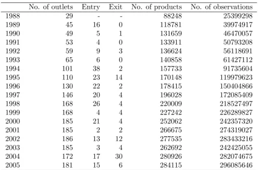
The data used in this paper is collected by Nikkei Digital Media Inc. The frequency of the data is daily and the sample period is from 1988 to 2005. The number of outlets covered as of 2005 is 181. Individual products are identified by their JAN (Japanese Article Number) Code and the total number of different products sold in 2005 is about 284,000. The total number of observations for 2005 is about 290 million (defined as the no. of articles × no. of outlets × no. of days), while the total for the entire sample period is approximately 2.9 billion observations.
[Insert Tables 1 and 2]
Tables 1 and 2 show the number of outlets and products for each year, as well as the turnover in outlets and products during the sample period. The number of outlets that are included in the dataset throughout the entire sample period is 17. The number of products sold by those 17 outlets in 1989 is approximately 230,000 and has subsequently risen steadily, reaching roughly 460,000 in 2004. During this period, tens of thousands of products were newly launched each year, but about the same number of products were also withdrawn. The ratio of the number of newly launched products relative to existing products was about 35 percent, while the withdrawal rate was about 30 percent, indicating that the turnover in products was quite rapid.
2Looking at the symmetry and asymmetry on a long time scale for each year, we find that at the beginning of the 1990s, the probability of a price rise was significantly larger than the probability of a price fall. This period represents the final phase of the asset price bubble and at this time, the consumer price index was also on an upward trend. The results here thus show that the exact opposite asymmetries occur in period of inflation and periods of deflation.
3 The Probability of Price Changes
Changes in selling prices at outlets reflect not only changes in regular prices, but also the effect of temporary sales. In order to remove the effect of such sales, we use the following filter. Let the selling price of a particular product at a particular outlet on day t be represented by ˆPit; then we define Pit as :
Pit≡ max{ ˆPit, ˆPit−1, . . . , ˆPit−k+1} (1) That is, P is the largest value of ˆP in the last k days. P coincides with the regular price under the assumption that (1) the selling price returns to the regular price on days when there is no temporary sales and (2) there are no temporary sales of a consecutive k days. We set k = 5 throughout the paper.
We then define the index showing the occurrence of price adjustment as
Iitd ≡( 1 if Pit6= Pit−d
0 if Pit= Pit−d (2)
If one or multiple price adjustments occur between day t − d and day t, then Iitd becomes 1. On the other hand, if no price adjustment occurs during this period, Itd is 0.
3.1 Heterogeity across products, outlets, and years
The upper panel of Figure 1 shows the distribution of the price change prob- ability, Pr(Iitd = 1), calculated by product and by outlet when d = 5. The horizontal axis represents the price change probability divided into 20 bins. The interval farthest to the right shows the (2−1/2, 1] bin, the adjacent one is the (2−2/2, 2−1/2] bin, followed by the (2−3/2, 2−2/2] bin, etc. The farther to the left, the stickier are the prices. For example, a price change probability of 1/8 means that the probability of its occurrence within a period of d days is 1/8, and with d = 5, prices are adjusted at a frequency of once in 40 days. The vertical axis shows the frequency. Note that, throughout the paper, we exclude products with a lifespan of less than 100 days in order to have sufficiently many price spells for each product.
[Insert Figure 1]
To begin with, looking at the distribution by product, we find that although it peaks at a probability of (2−5/2, 2−4/2], or (1/5.7, 1/4], the tails of the distri- bution are extremely long and the highest frequency can in fact be found in the
bin farthest to the left, where the price change probability is less than 1/724. This is a clear indication that there is huge heterogeneity between products in their price change probability. Looking at the distribution by outlet, we also find a wide dispersion of price adjustment probabilities, although this is not as great as in the distribution by product.
The middle panel of Figure 1 shows the cumulative distribution functions of the price change probability for various values of d. We see that the tail becomes thinner for larger d, but the difference is not significant, so we still have large heterogeneity even for the case of d = 20. The median of price duration is 67 days for the case of d = 5, and 95 and 135 days for d = 10 and 20, respectively. Finally, the bottom panel of Figure 1 presents the price change probability for each year. It shows that although the price change probability is almost stable from 1988 onward throughout the 1990s, a large increase is observed from 2000. One may suspect that this increase since 2000 was created by a substantial turnover in outlets (i.e., a large number of entries and exits) during that period. To remove this effect, we calculate the price change probability based only on the 17 outlets that existed throughout the entire sample period. But the result is the same as before. The fact that the price adjustment probability changes in each year implies that the stochastic process for prices is not invariant over time, so that it would be dangerous to examine the price change probability and the associated price change distributions without paying a particular attention to such a non-stationarity.
3.2 How to cope with heterogeneity
To deal with such heterogeneity across products and years in the price change probability, we do the following. First, we concentrate on the period from 1988 to 2002 unless otherwise mentioned, during which the price change probability was relatively stable. Second, we classify products into ten subgroups depending on the price change probability during the entire sample period. Specifically, we label products with a price change probability belonging to (1/2, 1] as G0. Similarly, those with a probability belonging to (1/4, 1/2] as G1, those with a probability belonging to (1/8, 1/4] as G2, etc. The tenth subgroup G9 comprises products with a probability of less than 1/512. G0 is the subgroup in which prices are the most flexible, maybe reflecting smallest menu costs. Progressing to G1, G2, etc., prices become increasingly stickier, maybe reflecting larger menu costs.
[Insert Table 3]
Table 3 shows a fraction of G0, G1, . . . , and G9 for each of the 26 product categories. Somewhat surprisingly, the table shows no substantial difference in the composition across product categories. For example, “frozen foods,” which is characterized by the highest price change probability among the 26 product categories, does not necessarily consist only of products with very flexible prices, such as G0 and G1: it also contains products with very sticky prices, such as G9. On the other hand, “stationery,” which is characterized by the lowest price change probability, contains products with very flexible prices, such as G0, G1, and G2, although the share of G9 is indeed outstanding, and significantly higher than in the other product categories. These facts have an important implication that the product category is not so useful in grouping products in terms of the price change probability; nevertheless, previous researches tend to assume that one can obtain a homogeneous set of products by making use of the product category. In this paper we shall not use it any more in grouping the products; we shall instead use the statistics we obtain from the data, including the probability of price changes, in identifying a set of homogeneous products.
[Insert Figure 2]
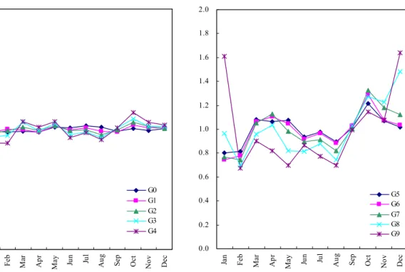
Figure 2 presents monthly seasonality of the price change probability for each of the product subgroups G0, G1, . . . , and G9. For example, the January figure for G0 represents the probability of price changes in January, which is calculated as the number of days with price changes in January divided by the total days in January, relative to the annual counterpart. We see in the figure that products with sticky prices, such as G7, G8, and G9, exhibit a strong monthly seasonality, while those with flexible prices, such as G0 and G1, do not show any significant seasonality. Given that the existence of seasonality is not consistent with state dependent pricing but consistent with some sort of time dependent, or more precisely, date dependent pricing, this result suggests that the latter is adopted, at least partially for those products with sticky prices.
4 Are Small Price Changes Rare?
4.1 Empirical strategy
Simple versions of menu cost models imply that there should not exist any small price changes. Based on this understanding, several researchers, including
Kashyap (1995), Carlton (1986), Midrigan (2006), and Lach and Tsiddon (2006), look for small price changes in price change distributions for the United States and Israel. They all find that the densities associated with small price changes are not zero, regarding this as evidence against the menu cost hypothesis.
However, the mere existence of non-zero densities for small price changes does not necessarily imply the non-existence of products whose prices are de- termined as described by menu cost models. To illustrate this, let us consider a situation in which all firms adopt state dependent pricing for all products, but each product differs in its menu cost and thus in its inactive range. Such a mixture of heterogeneous products with different menu costs and thus different inactive ranges would be able to create some (or even many) small price changes, which come only from products with relatively narrow inactive ranges.
How can we classify products into subgroups in which products within a group are homogeneous in terms of their inactive ranges? To show the method- ology we shall adopt in this paper, let us start by expressing state dependent pricing as
Iitd ≡( 0 if (1 + hi)
−1≤ Pit∗
Pit−d ≤ 1 + hi
1 otherwise (3)
where hirepresents the size of an inactive range for product i, which is of course closely related to the size of a menu cost, and Pit∗ is the target price for product i. In words, a price change occurs if and only if the actual price deviates from its target counterpart by more than hi. Moreover, it is assumed that when firms change prices, they completely eliminate a deviation from the target price, so that the gross inflation rate from t−d to t for product i, denoted by Πdit, satisfies
Πdit= Pit∗
Pit−d. (4)
This pricing rule, with an additional assumption that hi is sufficiently small relative to the volatility of the target price,3 implies
Iitd ≡( 0 if (1 + hi)
−1≤ Π∗d
it ≤ 1 + hi
1 otherwise (5)
and
Πdit= Π∗dit. (6)
3Under this assumption, Pit∗/Pit−dis almost equal to Pit∗/Pit−d∗ .
where Π∗dit, defined as Pit∗/Pit−d∗ , represents the gross inflation rate for the target price, which is assumed to have a symmetric distribution. Equation (5) gives the price change probability for product i as
Pr£Iitd = 1¤ = 1 − Pr £(1 + hi)−1≤ Π∗dit ≤ 1 + hi¤ (7) It should be noted that heterogeneity across products in terms of the price change probability comes from two sources; namely, heterogeneity in hi and heterogeneity in the volatility of Π∗dit. On the other hand, equation (6) has a useful implication about the tails of price change distributions:
Pr£Πdit≥ 1 + ξ | Iitd = 1¤ = Pr £Π∗dit ≥ 1 + ξ | Iitd = 1¤
Pr£Πdit≤ (1 + ξ)−1| Iitd = 1¤ = Pr £Π∗dit ≤ (1 + ξ)−1| Iitd = 1¤ (8) where ξ is a positive parameter satisfying ξ > hifor any product i. Furthermore, applying the Bayes’s theorem to the right hand side of equation (8) leads to
Pr£Πdit≥ 1 + ξ | Iitd = 1¤ = Pr£Π∗dit ≥ 1 + ξ
¤ Pr£Iitd = 1¤ Pr£Πdit≤ (1 + ξ)−1| Iitd = 1¤ = Pr£Π∗dit ≤ (1 + ξ)−1
¤
Pr£Iitd = 1¤ (9)
Equations (7) and (9) tell us the following procedure to collect products that are homogeneous in terms of hi. A key is to make use of information both on price change probabilities and on the tails of price change distributions. First of all, we collect products that satisfy the following two conditions simultaneously. Pr£Iitd = 1¤ = a (10) Pr£Πdit≥ 1 + ξ | Iitd = 1¤ = Pr £Πdit≤ (1 + ξ)−1 | Iitd = 1¤ = b (11) where a and b are parameters ranging between zero and unity. These two equations, together with equation (9), indicate that the products collected in this way should satisfy
Pr£Π∗dit ≥ 1 + ξ¤ = Pr £Π∗dit ≤ (1 + ξ)−1¤ = ab. (12) In other words, the products collected in this way should be homogeneous in terms of the volatility of the target price. Combined with the fact that the price change probability depends on hi and the volatility of the target price, this means that those products should be homogeneous even in terms of hi.
In the next subsection we shall collect products that are homogeneous win terms of hi to see whether the price change distributions have a dent at the vicinity of zero inflation. If we successfully find one, it implies that prices are determined as described by the menu cost hypothesis, at least for some portion of the products. On the other hand, if we fail to find a dent in the distributions, it is an evidence against state dependent pricing, and an evidence for time dependent pricing. If some (not necessarily all) firms adopt time dependent pricing in the sense of Calvo (1983), it would be possible that we find non- zero density for small price changes, which mainly come from firms with time dependent pricing.
Before proceeding to the empirical results, let us mention some possible limitations of our methodology. First, the above argument crucially depends on the assumption that hi is sufficiently small relative to the volatility of the target price. Equation (12) would not hold without this assumption. Then we would never be able to identify products that are homogeneous in terms of the volatility of the target price, so that those products collected using the proposed procedure are not necessarily homogeneous in terms of hi. This may not be a serious problem for those products with high price change probabilities, but could be a serious one for those products with very sticky prices.
Second, we have assumed in the above discussion that a price adjustment occurs if and only if the deviation of the actual price from the corresponding target level exceeds a threshold, as often assumed in menu cost models. How- ever, Caballero and Engel (2006) propose a model in which the probability of a price change increases with the deviation of the price from the target level, but only gradually (i.e., not discontinuously). If this is the case, it would not be surprising even if we observe non-zero density for small price changes. We will not be able to eliminate these small price changes even if we apply the above procedure.
4.2 Empirical results
We classify products by the price change probability (equation (10)) in subsec- tion 4.2.1, with the assumption that the volatility of target price is identical across products, and then classify products by the price change probability and the volatility of observed price changes (equations (10) and (11)) in subsection 4.2.2.
4.2.1 Grouping by the price change probability
Probability density functions Figure 3 shows f (Π5t | It5 = 1) for the 10 product subgroups. The sample period is 1988 to 2002, and the observations from all outlets are included. The horizontal axis represents 20 bins for the gross inflation rate, consisting of (0, 2−9/20),[2−9/20, 2−8/20), [2−8/20, 2−7/20), [2−7/20, 2−6/20), . . ., [2−1/20, 20/20), (20/20, 21/20], . . ., (28/20, 29/20], (29/20, ∞).
[Insert Figure 3]
The distribution for the subgroup G0, i.e., the subgroup with the most flexi- ble prices, shows that the densities for two bins at the center of the distribution, [0.96, 1) and (1, 1.03], are higher than those for the other bins.4 That is, the densities for small price changes are greater than those for large price changes. We see a similar regularity for the subgroup G1. However, we do not see such a single modal distribution for the other subgroups with prices being stickier than G1. For example, the distribution for the subgroup G2 has a dent at its center in that the densities associated with [0.96, 1) and (1, 1.03] are slightly smaller than the densities for the bins surrounding these two. We can see such a dent at the center of the distributions for G3, G4, and G5 as well.
To check the robustness of this finding, we conduct the same exercise as in Figure 3, but using different samples. First, we extract products whose prices are above 200 yen in order to see whether a dent at the center of a distribution is created not by menu costs, but by monetary indivisibility. Figure 4 clearly shows that this is not the case.
[Insert Figure 4]
Second, we change the sample period from 1988-2002 to 1988-2005. As we saw in Figure 1, the probability of price adjustments substantially increased in and after 2003. We are thus curious about how such heterogeneity in terms of the price change probability across years would affect price change distributions. Figure 5 shows a regularity that is quite different from what we saw in Figure 3; namely, densities associated with the two bins, [0.96, 1) and (1, 1.03], are now greater than others for the subgroups ranging from G0 to G7. In other words, small price changes are not rare any more for these subgroups. By scrutinizing the data, we can confirm that this is a direct consequence of heterogeneity of
4The bins [0.96, 1) and (1, 1.03] correspond to [2−1/20, 20/20) and (20/20, 21/20], respec- tively.
the price change probability across years. For example, those products which are classified into G3 have a similar distribution as in Figure 3 for the period of 1988-2002, but they exhibit a single modal distribution for the period of 2003- 2005, during which not only the probability of price changes increased, but also the likelihood of small price changes increased substantially for those products.5 The result of this exercise shows that heterogeneity across time, not to mention heterogeneity across products, could create a serious problem in detecting a dent at the vicinity of zero inflation.
[Insert Figure 5]
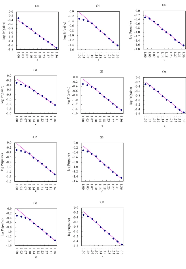
Cumulative distribution functions Figure 6 shows cumulative density func- tions, CDFs, of price changes for the 10 product subgroups. Figure 6.1 shows CDFs for the case of price decreases, i.e., Π < 1, where the vertical axis rep- resents log Pr(Π5 < c | I5 = 1) with c ≤ 1, and the horizontal axis represents the value of c. Similarly, Figure 6.2 shows CDFs for the case of price increases, Π > 1, and the vertical axis represents log Pr(Π5> c | I5= 1), where c ≥ 1.
[Insert Figure 6]
We can see in Figure 6.1 that every point of a CDF is on a straight line except two or three points from the right, which are close to Π = 1. Given that the horizontal axis is expressed in logarithm, and the vertical axis represents the log of CDF, this fact implies that the PDF and the CDF governing large price changes are given by the forms of
f (Π | I = 1) ∼ Π−α; (13)
F (Π | I = 1) ∼ Π−(α−1), (14)
where α is a positive parameter. A distribution with these forms of PDF and CDF is referred to as power law distribution or Pareto distribution, where α is called the power law exponent.6 An important feature of this form of distribu- tion is that it has a very long tail. Using the U.S. scanner data, Midrigan (2006) find that a price change distribution has tails fatter than those of a normal dis- tribution, and that density at the vicinity of zero inflation is greater than those
5An interpretation is that menu costs for these G3 products were very low in 2003-2005, leading to an increase in the price change probability as well as an increase in the likelihood of small price changes.
6See, for example, the appendix of Gabaix et al. (2006) or Gabaix (2007) for more on power law distributions.
of a normal distribution. Our finding is consistent with the first one, although it is in sharp contrast with the second one.
A careful examination of Figure 6.1 reveals that seven points from the left, namely points corresponding to c = 0.73, 0.75, 0.78, 0.81, 0.84, 0.87, 0.90, are on a straight line, but the remaining three points, namely those which correspond to c = 0.93, 0.96, 1.00, are below the straight line. This suggests a methodology to quantitatively evaluate distortions at the central part of a price change dis- tribution: we first fit a straight line for the seven points by an ordinary least squares regression, then extrapolate the line to the remaining three points, and finally obtain prediction errors, which is defined as predicted minus actual val- ues, as a measure for distortions of a distribution at the vicinity of zero inflation. The red lines shown in Figure 6.1, which are obtained in this way, indicate that actual values for the three points from the right tend to be smaller than the predicted ones, suggesting that small price changes are less likely to occur as compared with large price changes. The same method is applied to the case of price increases, and the result is presented in Figure 6.2.
[Insert Table 4]
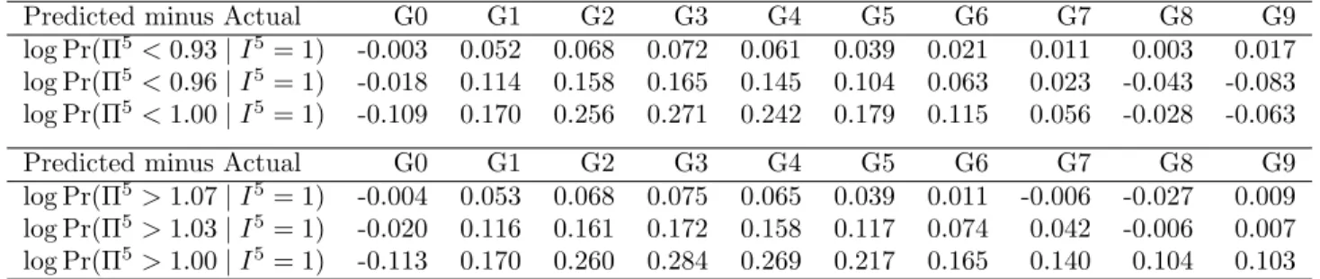
Table 4 presents estimates for distortions at the vicinity of zero inflation. For example, the number at the upper left corner, -0.003, represents how much the predicted value deviates from the actual one in terms of the third point from the right, namely log Pr(Π5< 0.93 | I5= 1), for the product subgroup G0. We can read from this table that predictions errors tend to be larger for G1 than for G0, and those for G2 are larger than those for G3, and so on, implying that the distortions become greater for those products with stickier prices. However, this relationship is not a monotonic one; Prediction errors tend to decrease with price stickiness for the product subgroups G4, G5, and so on, and finally those errors become very close to zero or even below zero for the products with very sticky prices, G8 and G9.7
7As we see in Figure 6.1, the slope of an estimated line, namely the power law exponent, tends to become smaller with price stickiness. This tendency is particularly clear for G6, G7, and G8. This implies that the variance of a distribution, which governs large price changes, becomes larger with price stickiness. This could explain, at least partially, why the prediction errors are so small for those products with sticky prices like G8 and G9.
4.2.2 Grouping by the price change probability and the volatility of the target price
To collect products whose price change distributions have long tails, we impose an additional constraint that
Pr£Π5it≥ 1 + ξ or Π5it≤ (1 + ξ)−1¤ > 0 (15) for each product subgroup. Figure 7 shows the price change distributions for the products collected in this way. The products that belong to G0 and satisfy the above condition are labeled as G0L; G1L, . . . , G9L are similarly defined. We set 1 + ξ = 21/2. The figures on the left hand side use the same horizontal axis as we did before for Figure 3 and so on, while the figures on the right hand side adopt a different scale for the horizontal axis in order to look more closely at price changes of larger magnitude.8
First, we find that the price change distribution for G0L has a single peak, indicating that small price changes occur even more often than larger ones. This is the same result as we saw in Figure 3, suggesting that menu costs are extremely small for those products with very flexible prices, or simply rejecting the menu cost hypothesis. Second, we clearly see a dent at the vicinity of zero inflation for the price change distributions of G2L, G3L, and G4L, as we did in Figure 3. Finally, as for products with very sticky prices, such as G6L, G7L, G8L, and G9L, we see a dent at the vicinity of zero inflation in their distributions: this can been seen more clearly in their CDFs presented in Figure 8. This has never been observed in Figures 3 nor 6, suggesting that we failed to detect a dent because of the mixture of products with different menu costs and thus different inactive ranges. Note that observed inactive ranges for these products are quite wide; for example, the densities between 0.76 and 1.32 are almost zero for G9L, indicating that price changes within ±30 percent are less likely to occur for such products with very sticky prices.
[Insert Figures 7 and 8]
8The horizontal axis for the figures on the right hand side represents 20 bins for the gross inflation rate, consisting of (0, 2−9/5),[2−9/5, 2−8/5), [2−8/5, 2−7/5), [2−7/5, 2−6/5), . . ., [2−1/5, 20/5), (20/5, 21/5], . . ., (28/5, 29/5], (29/5, ∞).
5 Symmetry/Asymmetry of Price Change Dis-
tributions
So far we have set d at d = 5. But one may wonder how price change distribu- tions would change when we choose different values for d. Note that changing the value of d is equivalent to changing time scale. In particular, we are inter- ested in how symmetry or asymmetry would be changed when we look at the data on a longer time scale.
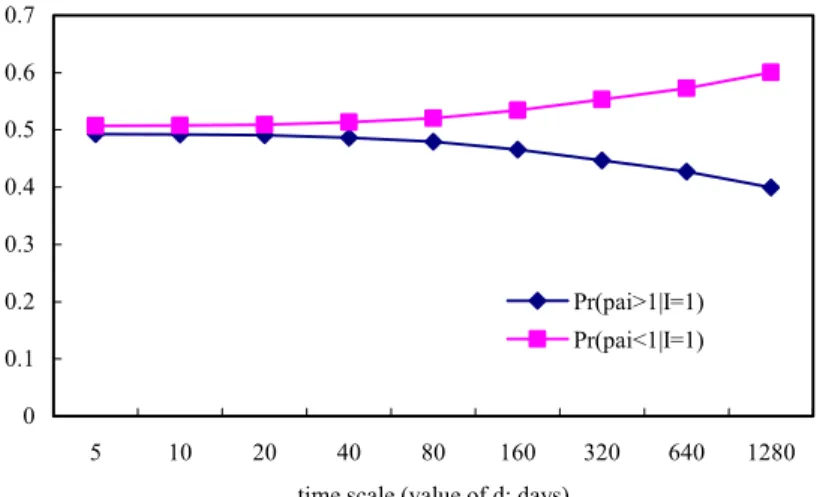
[Insert Figure 9]
Figure 9 presents the result of this exercise: we plot Pr(Πd > 1 | Id = 1) and Pr(Πd< 1 | Id= 1) for various values for d (d = 5, 10, 20, . . . , 1280). First, we can see that the two probabilities are both equal to 0.5 for d = 5 and d = 10, indicating that price change distributions are symmetric on a short time scale. This is consistent with the fact that most of the PDFs we saw in Figure 3 are symmetric. Progressing to longer time scales, however, the probability of a price decrease, Pr(Πd < 1 | Id = 1), monotonically increases: it reaches above 0.6 when d = 1280, indicating a substantial asymmetry.
Golosov and Lucas (2006) propose a model about firms’ pricing decisions in an environment with both idiosyncratic and aggregate productivity distur- bances. It would be safe to say that we observe the effects of idiosyncratic disturbances on price change distributions when we choose small values for d, such as 5 and 10 days, while we observe those of aggregate disturbances on price change distributions when we choose large values for d, such as 640 and 1280 days. If this is the case, the results presented in Figure 9 show that idiosyncratic disturbances are symmetric, which is consistent with the assumption adopted by Golosov and Lucas (2006), while aggregate disturbances, including monetary policy shocks, are strongly asymmetric.
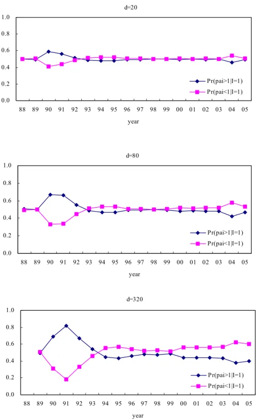
[Insert Figure 10]
Asymmetric distributions on a long time scale themselves might not be so surprising, but one may wonder why the probability of a price decrease (not a price increase) becomes higher on a longer time scale. This might be related to the fact that our sample period overlaps at least partially with the period when the Japanese economy experienced deflation. To investigate further on this possibility, we plot in Figure 10 the two probabilities, Pr(Πd> 1 | Id = 1) and Pr(Πd< 1 | Id= 1), for each year of our sample period, 1988-2005.
First, we see that the probability of a price decrease was higher than 0.5 from 2000 onward until 2005: we observe particularly strong asymmetry in 2004 and 2005. If we recall that the Japanese rate of inflation, measured either by the CPI or by the GDP deflator, was below zero during the period of 2000-2005, we may be allowed to interpret this asymmetry as reflecting deflation during this period. The second finding from Figure 10 is that there was another asymmetry at the beginning of the 1990s, in the sense that the probability of a price increase (rather than the probability of a price decrease) significantly exceeded 0.5. This period was a final stage of the asset price bubble in which the CPI inflation rate eventually started to rise fairly sharply. The observed asymmetry might have arisen from such an inflationary pressure in the Japanese economy.
6 Relationship between the Price Change Dis-
tribution and Price Duration
The probability of price adjustments and price change distributions could both potentially depend on past events. Among various types of history dependence, researchers have been interested in the dependence of the price change probabil- ity upon how long the time has passed since the last price change. For example, Campbell and Eden (2006) find from the US scanner data that the price change probability is inversely correlated with price duration, i.e., a decreasing haz- ard function. Similar results have been reported by Alvalez et al. (2005) for European countries.9
An important thing to note here is that price duration could be correlated not only with the price change probability, but also with the price change distri- bution conditional on the occurrence of a price change. The latter correlation is the main interest of this section. To our knowledge, there is no serious studies on the latter correlation as far as prices of goods and services are concerned.10
The menu cost hypothesis has clear implications about these two kinds of history dependence. First, the hazard function should be upward sloping. Under the assumption that the variance of the target price monotonically increases with
9These studies deal with prices for those products and services that are typically included in consumer price indexes, while other studies, such as Engle and Russell (1998) and Zhang et al. (2001), investigate history dependence for asset prices. For example, Zhang et al. (2001) estimate a hazard function for the IBM stock price, and find that it is not even monotonic, but is of an inverted U shape.
10However, there are several studies that investigate the relationship between asset price change distributions and price duration. See, for example, Russell and Engle (1998) that studies such a relationship using IBM stock prices.
time, the deviation of the actual price from the target price becomes larger as the time elapses since the last price adjustment. Thus the probability of price adjustment is an increasing function of price duration.
Second, the price change distribution should be independent of price dura- tion. According to a simple Ss rule, price adjustment occurs only when the deviation from the target price reaches s, and the new price is set at S, there- fore the price change always equals to S -s.11 There is no mechanism in such a simplified version of menu cost models that would yield a correlation between the price change distribution and price duration. More generally, the devia- tion of the actual price from the target price is a state variable in menu cost models, and when the value of this state variable meets a specific condition, price adjustment occurs. Put differently, if we were to gather instances of price adjustments, in each instance, the size of the deviation of the actual price from the target price should be identical. As long as firms base their decision on the magnitude of price adjustments in correspondence to the magnitude of the deviation, identical price change distributions should be observed, irrespective of how long the time have passed since the last price change.
6.1 Duration and the price change probability
We start by looking at the relationship between price duration and the prob- ability of price adjustments. We denote price duration as n and calculate the probability defined by
Pr[Itd= 1 | It−dd = It−2dd = · · · = It−ndd = 0, It−(n+1)dd = 1]. (16) for each product subgroup. Figure 11 presents the results: Figure 11.1 for the case of d = 5 and Figure 11.2 for the case of d = 20. The horizontal axis depicts nd, which express price duration by the number of days since the last price adjustment.12 As we see from Figure 11.1, there is a clear negative correlation between price duration and the price change probability for the product sub- group G0. Even for other subgroups, the price change probability is inversely correlated with price duration, except that there is a small spike at 20 days for these subgroups. A similar result is obtained in Figure 11.2. These results are consistent with the existing studies on the shape of hazard functions.
[Insert Figure 11]
11See, for example, Sheshinski and Weiss (1977).
12Note that we calculate the price change probability even for n = 0, i.e., Pr[Itd= 1 | It−dd = 1]. This differs from the usual hazard function which starts at n = 1.
6.2 Duration and the price change distribution
The observed negative correlation between price duration and the price change probability is obviously inconsistent with the menu cost hypothesis, but it has an even more unpleasant implication about the dynamic evolution of prices. That is, under the assumptions that (1) the variance of target prices increases with time, and that (2) price change distributions are independent of price duration, a decreasing hazard implies that the deviation of actual prices from target prices monotonically increases with time. Given that firms never allow actual prices to substantially deviate from target prices, either of the two assumptions must be violated. One possibility is that price change distributions are correlated with price duration in that large price changes become more likely to occur as the time passes since the last price adjustment.
[Insert Figure 12] To examine this possibility, we first calculate
log Pr[Πdt < c | It−dd = It−2dd = · · · = It−ndd = 0, It−(n+1)dd = 1] for c ≤ 1 (17) log Pr[Πdt > c | It−dd = It−2dd = · · · = It−ndd = 0, It−(n+1)dd = 1] for c ≥ 1 (18) for each product subgroup, with d being set at d = 5.13 And then we estimate distortions of price change distributions at the vicinity of zero inflation using the same method as in Section 4.2.1. Table 5 presents estimates for such distortions. If we look at the upper panel, which shows estimated distortions for Π < 1, we see almost no correlation between the estimated distortions and price duration for the subgroup G0 and G1. In other words, price change distributions are independent of price duration in terms of relative frequency of small and large price changes, which is consistent with the menu cost hypothesis. However, if we look at the columns for G2, G3, and G4 at the upper panel, we see a positive correlation between the estimated distortions and price duration. This tendency is more clearly seen at the lower panel, which shows results for Π > 1: for example, the estimated distortion for G4 increases from 0.051 at the duration of 10 days to 0.095 at the duration of 40 days, and finally to 0.228 at the duration of 70 days. In other words, as far as positive inflation is concerned, small (positive) price changes become less likely to occur relative to large (positive) price changes as the time elapses since the last price adjustment.
13Figures 12.1 and 12.2 show CDFs defined by (17) and (18) for product subgroup G4.
[Insert Table 5]
Together with the observed negative correlation between the price change probability and price duration (i.e., a decreasing hazard function), this result implies that although the price change probability declines the longer the price duration, once a price adjustment occurs, the price change is likely to be large. This could be interpreted as indicating that firms raise prices by a substantial amount in order to eliminate large deviations from target prices, which is an unavoidable consequence of the long absence of price adjustments. Moreover, it should be noted that there is a clear asymmetry between a price increase and decrease; namely, a large price increase is likely to occur after the long absence of price adjustments, while the same thing is not true for a large price decrease. These empirical results suggest that menu costs increase as the time passes since the last price adjustment.
7 Conclusion
This paper has empirically examined the menu cost hypothesis by analyzing the distribution of price changes using daily scanner data covering almost all products sold at about 200 Japanese supermarkets. We have arrived at the following findings. First, as implied by the menu cost hypothesis, small price changes were indeed rare. The price change distribution for products with sticky prices has a dent in the center. In contrast, no such dent can be observed in the price change distribution for products with flexible prices. Second, we find that the longer the time that has passed since the last price change, the higher is the probability that a large price change occurs. Combined with the fact that the price change probability is a decreasing function of the price duration, this means that although the price change probability decreases as the price duration increases, once a price adjustment occurs, the magnitude of such an adjustment is large. Third, while the price change distribution is symmetric on a short time scale, it is asymmetric on a long time scale, with the probability of a price decrease being significantly larger than the probability of a price increase. The asymmetry on a long time scale seems to be related to the deflation that the Japanese economy has experienced.
References
[1] Alvarez, L. J., P. Burriel, and I. Hernando (2005). “Do Decreasing Haz- ard Functions for Price Changes Make Sense?,” Working Paper No. 461, European Central Bank.
[2] Bils, M., and P. J. Klenow (2004). “Some Evidence on the Importance of Sticky Prices,” Journal of Political Economy 112(5), 947-985.
[3] Caballero, Ricardo J., and Eduardo M.R.A. Engel (2006). “Price Stickiness in Ss Models: Basic Properties,” MIT.
[4] Calvo, Guillermo A. (1983). “Staggered Prices in a Utility-Maximizing Framework,” Journal of Monetary Economics 12, 383-98.
[5] Campbell, J. R., and B. Eden (2006). “Rigid Prices: Evidence from U.S. Scanner Data,” Vanderbilt University.
[6] Carlton, D. W. (1986). “The Rigidity of Prices,” American Economic Re- view 76(4), 637-658.
[7] Dotsey, M., R. King, and A. Wolman (1999). “State-Dependent Pricing and the Genaral Equilibrium Dynamics of Money and Output,” Quarterly Journal of Economics 114(2), 655-690.
[8] Engle, Robert F., and Jeffrey R.Russell (1998). “Autoregressive Condi- tional Duration: A New Model for Irregularly Spaced Transaction Data,” Econometrica 66, 1127-1162.
[9] Gabaix, Xavier (2007), “Power Laws” in The New Palgrave Dictionary of Economics, 2nd Edition.
[10] Gabaix, X., P. Gopikrishnan, V. Plerou, and H. E. Stanley, “Institutional Investors and Stock Market Volatility,” Quarterly Journal of Economics 121, 461-504.
[11] Gagnon, E. (2005). “Price Setting Under Low and High Inflation: Evidence from Mexico,” Northwestern University.
[12] Golosov, M., and R. E. Lucas (2006). “Menu Costs and Phillips Curves,” MIT.
[13] Kackmeister, A. (2005). “Yesterday’s Bad Times are Today’s Good Old Times: Retail Price Changes in the 1890’s were Smaller, Less Frequent, and More Permanent,” Finance and Economics Discussion Series, Federal Reserve Board.
[14] Kashyap, A. K. (1995). “Sticky Prices: New Evidence from Retail Cata- logs,” Quarterly Journal of Economics 110(1), 245-274.
[15] Klenow, P. J., and O. Kryvtsov (2005). “State-Dependent or Time- Dependent Pricing: Does It Matter for Recent U.S. Inflation,” Stanford University.
[16] Lach, S., and D. Tsiddon (2005). “Small Price Changes and Menu Costs,” The Hebrew University of Jerusalem
[17] Midrigan, V. (2005). “Menu Costs, Multi-Product Firms, and Aggregate Fluctuations,” Ohio State University.
[18] Nakamura, E., and J. Steinsson (2007). “Five Facts about Prices: A Reeval- uation of Menu Cost Models,” Harvard University.
[19] Russell, Jeffrey R., and Robert F. Engle (1998). “Econometric Analysis of Discrete-Valued Irregularly-Spaced Financial Transactions Data Using a New Autoregressive Conditional Multinomial Model,” UCSD Economics Discussion Paper 98-10.
[20] Sheshinski, E., and Y. Weiss (1977). “Inflation and Costs of Price Adjust- ment,” Review of Economic Studies 44(2), 287-303.
[21] Zhang, Michael Yuanjie, Jeffrey R. Russell, and Ruey S. Tsay (2001). “A Nonlinear Autoregressive Conditional Duration Model with Applications to Financial Transaction Data,” Journal of Econometrics 104, 179-207.
Table 1: Number of Outlets, Products, and Observations
No. of outlets Entry Exit No. of products No. of observations
1988 29 - - 88248 25399298
1989 45 16 0 118781 39974917
1990 49 5 1 131659 46470057
1991 53 4 0 133911 50793208
1992 59 9 3 136624 56118691
1993 65 6 0 140858 61427112
1994 101 38 2 157733 91735604
1995 110 23 14 170148 119979623
1996 130 22 2 178415 150404866
1997 146 20 4 196028 172085409
1998 168 26 4 220009 218527497
1999 168 4 4 227242 226289827
2000 185 21 4 252062 242357320
2001 185 2 2 266675 274319027
2002 186 13 12 277535 283433216
2003 185 3 4 262692 242425055
2004 172 17 30 280926 282074675
2005 181 15 6 284115 296085646
Table 2: Turnover of Products in the 17 Outlets
Number of products Entry Exit Entry rate Exit rate in the 17 outlets
1989 231942 80107 73882 0.345 0.319
1990 242605 84545 78180 0.348 0.322
1991 231488 67063 71559 0.290 0.309
1992 221828 61899 63364 0.279 0.286
1993 222170 63706 64353 0.287 0.290
1994 260540 102723 72713 0.394 0.279
1995 313019 125192 91897 0.400 0.294
1996 343012 121890 101909 0.355 0.297
1997 380912 139809 117468 0.367 0.308
1998 409046 145602 133590 0.356 0.327
1999 422121 146665 142888 0.347 0.339
2000 440935 161702 150383 0.367 0.341
2001 439873 149321 149506 0.339 0.340
2002 450879 160512 158003 0.356 0.350
2003 425856 132980 147450 0.312 0.346
2004 466156 187750 167677 0.403 0.360
Table 3: Price Change Probability by Product Category
G0 G1 G2 G3 G4 G5 G6 G7 G8 G9 Median of the probability
豆腐・納豆・コンニャク 0.038 0.090 0.137 0.132 0.090 0.061 0.037 0.021 0.009 0.385 0.067
漬物・惣菜 0.032 0.079 0.134 0.130 0.100 0.064 0.038 0.018 0.006 0.397 0.053
水産練り製品・チルド半製品 0.025 0.108 0.177 0.143 0.092 0.053 0.029 0.013 0.005 0.356 0.082
畜肉加工品 0.014 0.064 0.137 0.139 0.103 0.064 0.038 0.019 0.006 0.418 0.046
乳製品・豆乳類 0.015 0.084 0.158 0.141 0.095 0.053 0.029 0.014 0.005 0.405 0.071 チルドデザード 0.043 0.107 0.165 0.136 0.082 0.040 0.019 0.007 0.002 0.400 0.097
飲料 0.023 0.073 0.150 0.139 0.096 0.051 0.024 0.010 0.003 0.431 0.068
乾物・めん類 0.003 0.047 0.140 0.142 0.106 0.071 0.042 0.022 0.009 0.420 0.036
調味料・甘味料 0.003 0.058 0.141 0.131 0.097 0.064 0.039 0.020 0.008 0.438 0.037
即席食品 0.006 0.081 0.183 0.157 0.103 0.054 0.026 0.011 0.004 0.375 0.070
缶詰・瓶詰 0.003 0.060 0.160 0.158 0.123 0.074 0.039 0.017 0.005 0.361 0.047
パン・もち 0.045 0.098 0.136 0.118 0.090 0.061 0.036 0.018 0.007 0.391 0.062
ジャム・スプレッド 0.006 0.070 0.138 0.122 0.090 0.058 0.033 0.016 0.006 0.461 0.035 コーヒー・紅茶・緑茶 0.009 0.113 0.179 0.144 0.096 0.053 0.026 0.012 0.004 0.365 0.074
菓子 0.009 0.047 0.134 0.135 0.093 0.050 0.027 0.012 0.004 0.489 0.033
酒類 0.011 0.079 0.132 0.112 0.086 0.051 0.025 0.009 0.003 0.491 0.053
ベビーフード・穀類 0.016 0.104 0.132 0.111 0.088 0.053 0.025 0.009 0.003 0.459 0.046
冷凍食品 0.016 0.121 0.218 0.158 0.087 0.042 0.021 0.008 0.003 0.326 0.110
アイスクリーム・氷 0.046 0.111 0.172 0.129 0.079 0.037 0.018 0.008 0.003 0.397 0.094 衛生用品・洗剤 0.010 0.128 0.223 0.147 0.085 0.044 0.020 0.008 0.002 0.334 0.099 化粧品・フレグランス 0.042 0.122 0.140 0.111 0.094 0.055 0.026 0.008 0.001 0.402 0.049 医療関連品・雑貨 0.005 0.044 0.104 0.113 0.107 0.078 0.046 0.024 0.009 0.471 0.016 キッチン消耗品 0.003 0.044 0.117 0.130 0.110 0.072 0.042 0.018 0.006 0.459 0.027 ステーショナリー 0.001 0.009 0.036 0.064 0.088 0.071 0.043 0.018 0.005 0.665 0.001 ペットフード・サニタリー 0.017 0.138 0.187 0.122 0.083 0.048 0.023 0.009 0.002 0.372 0.082 0.028 0.231 0.295 0.135 0.079 0.029 0.011 0.001 0.000 0.189 0.001
Table 4: Prediction Errors by Product Subgroup
Predicted minus Actual G0 G1 G2 G3 G4 G5 G6 G7 G8 G9
log Pr(Π5< 0.93 | I5= 1) -0.003 0.052 0.068 0.072 0.061 0.039 0.021 0.011 0.003 0.017 log Pr(Π5< 0.96 | I5= 1) -0.018 0.114 0.158 0.165 0.145 0.104 0.063 0.023 -0.043 -0.083 log Pr(Π5< 1.00 | I5= 1) -0.109 0.170 0.256 0.271 0.242 0.179 0.115 0.056 -0.028 -0.063
Predicted minus Actual G0 G1 G2 G3 G4 G5 G6 G7 G8 G9
log Pr(Π5> 1.07 | I5= 1) -0.004 0.053 0.068 0.075 0.065 0.039 0.011 -0.006 -0.027 0.009 log Pr(Π5> 1.03 | I5= 1) -0.020 0.116 0.161 0.172 0.158 0.117 0.074 0.042 -0.006 0.007 log Pr(Π5> 1.00 | I5= 1) -0.113 0.170 0.260 0.284 0.269 0.217 0.165 0.140 0.104 0.103
Table 5: Prediction Errors by Price Duration Predicted minus actual values for
log Pr[Πdt < 0.93 | It−dd = · · · = It−ndd = 0, It−(n+1)dd = 1]
Duration [days] G0 G1 G2 G3 G4
10 0.043 0.061 0.069 0.066 0.029
15 0.046 0.064 0.071 0.075 0.039
20 0.047 0.067 0.075 0.081 0.049
25 0.048 0.068 0.074 0.090 0.080
30 0.045 0.065 0.067 0.080 0.062
35 0.048 0.066 0.074 0.081 0.061
40 0.045 0.068 0.077 0.090 0.047
45 0.043 0.070 0.080 0.095 0.057
50 0.043 0.071 0.085 0.098 0.075
55 0.038 0.067 0.081 0.105 0.074
60 0.037 0.065 0.076 0.093 0.045
65 0.039 0.064 0.079 0.097 0.060
70 0.032 0.065 0.081 0.091 0.075
Predicted minus actual values for
log Pr[Πdt > 1.07 | It−dd = · · · = It−ndd = 0, It−(n+1)dd = 1]
Duration [days] G0 G1 G2 G3 G4
10 0.055 0.064 0.066 0.065 0.051
15 0.060 0.079 0.086 0.092 0.087
20 0.061 0.080 0.091 0.100 0.085
25 0.061 0.073 0.079 0.081 0.037
30 0.064 0.078 0.087 0.089 0.037
35 0.065 0.080 0.096 0.101 0.057
40 0.068 0.085 0.104 0.124 0.095
45 0.072 0.090 0.116 0.149 0.128
50 0.077 0.087 0.114 0.139 0.096
55 0.074 0.082 0.103 0.122 0.083
60 0.077 0.083 0.101 0.135 0.132
65 0.083 0.087 0.112 0.163 0.167
70 0.088 0.091 0.115 0.193 0.228
Figure 1: Price Change Probability by Product, Outlet, and Year
Distribution of the price adjustment probability: d=5
0.0 0.1 0.2 0.3 0.4
1/512 1/256 1/128 1/64 1/32 1/16 1/8 1/4 1/2 1
Product Outlet
The price adjustment probability in 1988-2005
0.0 0.1 0.2 0.3 0.4
1988 1989 1990 1991 1992 1993 1994 1995 1996 1997 1998 1999 2000 2001 2002 2003 2004 2005
All outlets 17 outlets
CDFs of the price adjustment probability for various time horizons
0.0 0.1 0.2 0.3 0.4 0.5 0.6 0.7 0.8 0.9 1.0
1/512 1/256 1/128 1/64 1/32 1/16 1/8 1/4 1/2 1
d=5 d=10 d=20
Figure 2: Monthly Seasonality of the Price Change Probability
0.0 0.2 0.4 0.6 0.8 1.0 1.2 1.4 1.6 1.8 2.0
Jan Feb Mar Apr May Jun Jul Aug Sep Oct Nov Dec
G0 G1 G2 G3 G4
0.0 0.2 0.4 0.6 0.8 1.0 1.2 1.4 1.6 1.8 2.0
Jan Feb Mar Apr May Jun Jul Aug Sep Oct Nov Dec
G5 G6 G7 G8 G9

![Table 5: Prediction Errors by Price Duration Predicted minus actual values for log Pr[Π d t < 0.93 | I t−dd = · · · = I t−ndd = 0, I t−(n+1)dd = 1] Duration [days] G0 G1 G2 G3 G4 10 0.043 0.061 0.069 0.066 0.029 15 0.046 0.064 0.071 0.075 0.039 20 0.047](https://thumb-ap.123doks.com/thumbv2/123deta/5651019.6490/26.892.250.668.285.604/table-prediction-errors-duration-predicted-actual-values-duration.webp)