T itle T he Impact of T axes and T ransfers on S kill Premium
A uthor(s ) T akahashi, S huhei; Y amada, K en
C itation K IE R D iscussion Paper (2017), 976: 1-31
Is s ue D ate 2017-08
UR L http://hdl.handle.net/2433/228361
R ig ht
T ype R esearch Paper
KIER DISCUSSION PAPER SERIES
KYOTO INSTITUTE
OF
ECONOMIC RESEARCH
KYOTO UNIVERSITY
KYOTO, JAPAN
Discussion Paper No.976
“
The Impact of Taxes and Transfers on Skill Premium
”
Shuhei Takahashi Ken Yamada
The Impact of Taxes and Transfers on
Skill Premium
∗
Shuhei Takahashi
†Ken Yamada
‡August 2017
Abstract
The level of wage inequality has varied across advanced industrial countries. One of
the main reasons has been a significant difference in the skill wage premium. This study
analyzes the impact of taxes and transfers on the skill wage premium and social welfare in
the context of a heterogeneous-agents incomplete-markets model, in which the population
consists of skilled workers and unskilled workers, and the production technology exhibits
capital-skill complementarity. The analysis indicates that a significant fraction of the
dif-ference in the skill wage premium between the United States and Japan can be accounted
for by differences in the tax system.
KEYWORDS: Skill premium; capital-skill complementarity; incomplete markets; capital
income taxation; composition effect.
JELCLASSIFICATION: E13, E24, E62, H24, J31.
∗We have benefited from comments and discussions with Sagiri Kitao, Toshihiko Mukoyama, and
numer-ous seminar and conference participants at Graduate Institute for Policy Studies, Hitotsubashi University, Kansai University, Keio University, Asian and European Meetings of the Econometric Society, DSGE/Macroeconomics and Econophysics Workshop, International Conference of the Society for Computational Economics, Tokyo La-bor Economics Workshop. We gratefully acknowledge financial support from JSPS KAKENHI grant numbers 15H06304, 16H02026, and 16H03626.
†Institute of Economic Research, Kyoto University. Phone: +81 (0)75 753 7153, Fax: +81 (0)75 753 7193,
Email:[email protected]
1
Introduction
The level of wage inequality has varied widely across advanced industrial countries (Krueger,
Perri, Pistaferri, and Violante, 2010). One of the main reasons for this has been a significant
difference in the skill wage premium, defined as the ratio of the average wage of college
gradu-ate workers to that of non-college gradugradu-ate workers. When the United Stgradu-ates and Japan, two of
the largest economies in the world, are compared, the variance of the log hourly wage was 47
percent higher in the United States than in Japan in the year 2000, while the college wage
pre-mium was 26 percent higher in the United States than in Japan (Heathcote, Perri, and Violante,
2010;Lise, Sudo, Suzuki, Yamada, and Yamada,2014).
Despite the large difference in the skill wage premium between the United States and Japan,
it would be fair to say that the difference in the level of technology or the share of the skilled
population was insignificant around the year 2000. In fact, the shares of population with tertiary
education were 36.5 percent in the United States and 33.6 percent in Japan in the year 2000
(OECD, 2015). The difference in the skill wage premium between the two countries cannot
simply be explained by differences in those supply and demand factors. In this study, we focus
on the impact of institutional differences between the two countries.
In particular, we examine the extent to which the difference in the skill wage premium
between the United States and Japan can be accounted for by differences in the tax system.
Interestingly, there was a notable difference in the tax rate on capital income between the two
countries around the year 2000, while there was no difference in the tax rates on consumption
or labor income, as detailed in the next section. In this study, we develop a general equilibrium
model, in which taxes and transfers affect the labor market equilibrium through a shift in the
supply of and demand for physical capital, as well as a shift in the relative supply of and demand
for skilled labor.
We consider a heterogeneous-agents incomplete-markets model, in which the population
consists of skilled workers and unskilled workers, and the production technology exhibits
capital-skill complementarity. Capital-capital-skill complementarity is a fundamental source of educational
wage differentials in a modern economy. We calibrate the model to the U.S. economy and
Japanese tax system on the skill wage premium and social welfare. We find that the skill wage
premium declines from 1.75 to 1.63 in the heterogeneous-agents incomplete-markets model as
a consequence of a change in policy that raises the tax rate on capital income and spends the
incremental revenue on transfers to households. The magnitude of this reduction corresponds
to 42 percent of the actual difference in the skill wage premium between the two countries. We
show that 72 percent of the reduction in the skill wage premium is attributable to the
equilib-rium effect with respect to a change in the relative marginal product, while the remaining 28
percent is attributable to the mechanical effect with respect to a change in the relative average
productivity. We further show that such a change in tax policy, which reduces persistent wage
differentials between skilled workers and unskilled workers, can effectively improve social
wel-fare.
This paper is closely related to the quantitative macroeconomic literature on the role of
taxes and transfers in the heterogeneous-agents incomplete-markets model of Huggett (1993)
andAiyagari(1994), extended to allow for endogenous labor supply. Among others,Flodén and
Lindé(2001) andAlonso-Ortiz and Rogerson(2010) focus on labor income taxes and transfers,
Nakajima and Takahashi (2016) focus on consumption taxes and transfers, and Aiyagari and
McGrattan(1998) andFlodén(2001) focus on government debt and transfers. We extend their
models by incorporating two types of labor that differ in the degree of substitution for capital and
focus mainly on capital income taxes and transfers. Slavík and Yazici(2016) use a model similar
to ours to examine the causes of changes in the skill wage premium over time in the United
States. In contrast, our analysis contributes to understanding the role of taxes and transfers in
accounting for cross-country differences in the skill wage premium. In this regard, this study
is an extension of the work by Prescott (2004) and Alonso-Ortiz and Rogerson (2010), who
examine the role of taxes and transfers in accounting for cross-country differences in labor
supply and productivity, respectively. In addition, our analysis contributes to understanding
differences in quantitative predictions regarding the impact of taxes and transfers between the
heterogeneous-agents incomplete-markets model and the representative-agent model.
The rest of the paper proceeds as follows. Section2compares the skill wage premium and
the equilibrium allocation. Section 4 discusses the measurement and decomposition of the
impact of taxes and transfers on the skill wage premium. Section 5describes the calibration
procedure and provides quantitative results on the skill wage premium and social welfare. The
final section summarizes and concludes.
2
US-Japan Comparison
We compare the skill wage premium and the tax system between the United States and Japan.
Figure 1: The skill wage premium in the United States and Japan
1.4 1.5 1.6 1.7 1.8
1995 2000 2005
US Japan Japan, adjusted
2.1
Differences in skill premium
The skill wage premium has been significantly higher in the United States than in Japan. Figure
1illustrates the skill wage premium between the years 1995 and 2005 in the United States and
between the years 1996 and 2006 in Japan. The data used in the analysis are from the Current
Population Survey (CPS) for the United States and the Employment Status Survey (ESS) for
Japan. The ESS is the most comparable household survey to the CPS for the purpose of the
analysis here, and has been conducted every five years in Japan by the Ministry of Internal
Affairs and Communications. We select the sample and construct variables in the same way as
Heathcote, Perri, and Violante(2010) for both countries and calculate the skill wage premium
for men and women aged 25 to 60. In the calculation, four-year college graduates are classified
was on average 1.75 in the United States and 1.44 in Japan.
The difference in the skill wage premium cannot be explained simply by differences in the
composition of the workforce between the two countries. First of all, the supply of skilled
labor was similar between the two countries relative to other OECD countries, and, if anything,
greater in the United States than in Japan. During the period, the share of the skilled population
was on average 29 percent in the United States and 22 percent in Japan. Moreover, even when
we reweight the Japanese sample such that it has the same distribution of age, sex, and education
as the U.S. sample using the DiNardo, Fortin, and Lemieux (1996) method, the skill wage
premium remains almost unchanged (Figure1).1
The difference in the skill wage premium has persisted for a long time between the two
countries. Educational wage differentials were consistently greater in the United States than
in Japan from the late 1960s to the 1980s (Katz, Loveman, and Blanchflower, 1995). The
skill wage premium has increased substantially in the United States in recent years, but the
magnitude of the increase over time has been small relative to the magnitude of the difference
in the skill wage premium between the two countries (Figure1).
2.2
Differences in the tax system
The capital income tax rate has been significantly higher in Japan than in the United States.
Trabandt and Uhlig(2011) calculate average marginal tax rates in the United States and many
European countries for the years 1995 to 2007. Gunji and Miyazaki(2011) provide comparable
average marginal tax rates in Japan during the corresponding period.2 Interestingly, during
the period, the capital income tax rate was on average 52 percent in Japan as opposed to 36
percent in the United States, while the consumption and labor income tax rates were on average
5 percent and 28 percent, respectively, in both countries. Among the countries analyzed in
Trabandt and Uhlig (2011), the capital income tax rate was near the average in the United
States and highest in Japan. Importantly, there was not much difference in the progressivity of
1Alternatively, even when we adjust for differences in the age, sex, and education composition of the workforce
across countries in a way similar toKrusell, Ohanian, Rios-Rull, and Violante(2000), who adjust for changes in the workforce composition over time, the difference in the skill wage premium mostly still remains.
2We adjust the results ofGunji and Miyazaki(2011) on the labor and capital income tax rates in Japan in a way
labor income taxes between the two countries during the period (See the OECD tax database
for details). A key feature of the Japanese tax system is the higher rate of capital income taxes
due in large part to the higher rate of corporate tax. Therefore, in the subsequent analysis, we
focus mainly on the impact of a change in policy that raises the tax rate on capital income on
the skill wage premium.
3
The Model
We consider the heterogeneous-agents incomplete-markets model, which is an extension of the
model inAlonso-Ortiz and Rogerson(2010), who incorporate labor income taxes and transfers
into the heterogeneous-agents incomplete-markets model ofChang and Kim(2007). Our model
differs from theirs in that the population consists of skilled workers and unskilled workers,
and the production technology exhibits capital-skill complementarity. The difference between
skilled workers and unskilled workers lies in the degree of substitution for capital.3 We consider
an extended version of the model, in which the productivity process differs between skilled
workers and unskilled workers in Appendix A.1. We present a representative-agent version of
the model in AppendixA.2.
3.1
Households
The economy is populated by a continuum of infinitely-lived agents of unit mass who are either
skilled or unskilled indexed by j ∈ {S,U}. Preferences are described by:
Et
∞
Õ
t=τ
βt−τUj(ct,ht), (1)
where β is the discount factor, ct consumption, and ht hours worked in periodt. Following
Alonso-Ortiz and Rogerson(2010), we specify the instantaneous utility function to be:
Uj(ct,ht)=lnc−ψjht for j ∈ {S,U}. (2)
3Our model shares a similar feature with the heterogeneous-agents incomplete-markets model inSlavík and
We assume indivisible labor, i.e. ht ∈ n
0,hj o
, and focus on the employment decision, which is
shown to be important in accounting for cross-country differences in productivity (Alonso-Ortiz
and Rogerson,2010).
Each household earnsxtwjtht, according to idiosyncratic shocks to productivityxt, the mar-ket wage ratewjt, and hours worked ht, and receives lump-sum transfers from the government to each household ft. Productivity evolves stochastically according to the transition probability function π(x′|x)=Pr(xt+1≤ xt|xt=x). We specify the idiosyncratic productivity process to be the first-order autoregressive process:
lnxt= ̺lnxt−1+ǫt, (3)
whereǫ is normally distributed with meanνand standard deviationς. We adjustνto normalize
the average idiosyncratic productivity to unity, i.e.,E(xt)=1, as in the analysis ofAiyagari and
McGrattan(1998). Each household can save but face a borrowing constraint: at+1 ≥0, where
assetsat consist of physical capital and government debt. The budget constraint can be written as:
(1+τc)ct=(1−τn)xtwjtht+[1+(1−τk)rt]at−at+1+ ft, (4)
ct≥0, at+1≥0, ht ∈
n
0,hj o
,
wherert is the rental price of capital. A key feature of the heterogeneous-agents incomplete-markets model is that households adjust their savings and labor supply to self-insure against
idiosyncratic shocks to their productivity under the borrowing constraint.
We now consider a recursive equilibrium. We denote by VE the present value of
house-hold utility when being employed, VN the present value of household utility when not being
employed, andξ(ea,x,j)is the distribution of households. Throughout the paper, the squiggles
denote normalization byY for detrending. The value of employment can be expressed as:
VE(ea,x,j)=max e
c,ea′
n
lnec−ψjhj+βE[V(ea′,x′,j)|x] o
subject to:
(1+τc)ec+(1+g)ea′=(1−τn)xwjhj+[1+(1−τk)r]ea+ ef, ec≥0, ea′≥0,
andξ′=T (ξ), where T denote a transition operator forξ. The value of non-employment can be expressed as:
VN(ea,x,j)=max
c,a′ {lnec+β
E[V(ea′,x′,j)|x]} (6)
subject to:
(1+τc)ec+(1+g)ea′=[1+(1−τk)r]ea+ ef, ec≥0, ea′≥0, andξ′=T (ξ). The labor supply decision can then be described by:
V(ea,x,j)=maxVE(ea,x,j),VN(ea,x,j) . (7)
A set of decision rules for consumption, hours worked, and asset holdings can be derived as
the solution to this problem. We denote byec(ea,x,j), h(ea,x,j), andea′(ea,x,j)the decision rules
for consumption, hours worked, and asset holdings, respectively.
3.2
Firms
Production in the economy is summarized by an aggregate functionYt=F(NSt,NUt,KEt,KSt;zt), where NSt is skilled labor input, NUt unskilled labor input, KEt equipment capital input, KSt structures capital input, and zt a measure of labor-augmenting technology in period t. We assume that final goods are produced by perfectly competitive firms.
We assume a constant returns-to-scale technology and specify the production function to be:
F (NSt,NUt,KEt,KSt;zt)=KStα n
µ(ztNUt)σ+(1−µ)
λKEtρ +(1−λ) (ztNSt)ρ σ
ρ
o1−α σ
. (8)
Labor-augmenting technology exhibits a deterministic trend: zt+1=(1+g)zt, whereg > 0 is the growth rate of technology. The share parameters are 0 ≤ µ, λ ≤ 1, and the substitution
by 1/ (1−ρ), while the elasticity of substitution between unskilled labor and the skilled
labor-capital composite is 1/ (1−σ). The degree of diminishing marginal product differs between
skilled labor and unskilled labor wheneverσ, ρ. Production technology exhibits capital-skill complementarity ifσ > ρ(Krusell, Ohanian, Rios-Rull, and Violante,2000).
Profit maximization is achieved by equating factor prices with the values of the marginal
products of inputs:
e
wSt = (1−α) (1−µ) (1−λ)Ke
ασ 1−α
St
λKeEtρ +(1−λ) (eztNSt)ρ σ−ρ
ρ
eztρNStρ−1, (9)
e
wUt = Ke
ασ 1−α
St (1−α)µez
σ
t NUtα−1, (10)
rEt = (1−α) (1−µ)Ke
ασ 1−α
St h
λKeEtρ +(1−λ) (eztNSt)ρ iσ−ρ
ρ
λKeEtρ−1−δS, (11)
rSt = αKeSt−1−δU, (12)
where δE and δS are the depreciation rates of equipment and structures, respectively. Capital equipment and structures are equivalent for households; thus, rE =rS =r at the equilibrium. None of the tax rates appears in the profit-maximizing conditions (9)–(12). Basically, taxation
does not play a significant role for the determination of factor prices in a partial equilibrium
model. In a general equilibrium model, however, capital income taxation reduces the stock of
capital and alters the relative marginal product of skilled labor, thereby influencing the skill
wage premium.
3.3
Government
We assume that the government levies proportional taxes and spends part of the tax revenue on
lump-sum transfers to households, as in many previous studies (e.g.,Flodén and Lindé, 2001;
Prescott, 2004;Alonso-Ortiz and Rogerson, 2010). When the government levies proportional
taxes on consumption, labor income, and capital income at rates τc, τn, and τk, respectively, and spends the tax revenue on government consumptionGt, lump-sum transfersFt, and interest payments on government debt Bt, the government budget constraint can be written as:
whereCtis aggregate household consumption. The government budget constraint can be rewrit-ten as:
e
G+Fe+rBe=Be′− (1+g)Be+τcCe+τn(ewSNS+weUNU)+τkr
e
KE+KeS+Be
. (13)
We assume thatGeandBeare exogenously given.
3.4
Equilibrium
The equilibrium of the economy is characterized as follows. Given policies nGe,Be, τc, τn, τk,Fe o
and initial conditions {z0, ξ0}, a stationary competitive equilibrium is a set of value functions
VE(ea,x,j),VN(ea,x,j),V(ea,x,j) , a set of decision rules for consumption, hours worked, and
asset holdings {ec(ea,x,j),h(ea,x,j),ae′(ea,x,j)}, aggregate inputs nNS,NU,KeE,KeS o
, price system
{weS,weU,r}, and a law of motion for the distributionξ′=T (ξ)such that: the decision rules and the value functions solve the household’s problem; aggregate inputs solve the firm’s problem;
the government budget is balanced; the capital market clears, i.e.,KeE′ +KeS′+Be′=∫ ea′(ea,x,j)dξ; labor markets clear, i.e.,NS=
∫
{j=S}xh(ea,x,j)dξandNU =
∫
{j=U}xh(ae,x,j)dξ; the final goods
market clears, i.e.,∫ {ec(ea,x,j)+ea′(ea,x,j)}dξ=F
NS,NU,KeE,KeS;ez
+(1−δE)KeE+(1−δS)KeS; and individual and aggregate behaviors are consistent for allA0⊂ AandX0⊂ X, i.e.,ξ′ A0,X0,j= ∫
A0,X0
n∫
A,X✶a′=a(ea,x,j)dπ(x′|x)dξ
o
dea′dx′.
4
Skill Premium
The equilibrium skill wage premium is defined as:
ωha≡ wSNS/HS wUNU/HU =
wS
wU
NS/HS
NU/HU
, (14)
where Hj is the aggregate labor supply of a group j, i.e., Hj = ∫
jh(ea,x,j)dξ for j ∈ {S,U}. The ratio of the market wage for skilled labor to the market wage for unskilled labor,wS/wU,
represents the relative marginal product. The ratio of the aggregate labor input to the
thus, the ratio of NjHj between the two groups represents the relative average productivity. The skill wage premium is determined by the product of the relative marginal product and the
relative average productivity, and increases with a rise in the relative marginal product and the
relative average productivity.
Effects on skilled and unskilled workers When we compare two countries with different tax
systems, the difference in the skill wage premium can be written as:
∆lnωha =∆ln
wSNS
HS
| {z }
effect on skilled
−∆ln
wUNU
HU
| {z }
effect on unskilled
. (15)
The first term is the difference in the average wage of skilled workers, while the second term
is the difference in the average wage of unskilled workers. We refer to the former as the effect
on skilled workers and the latter as the effect on unskilled workers. Naturally, the difference in
the skill wage premium is proportional to the difference in the average wage of skilled workers,
while it is inversely proportional to the difference in the average wage of unskilled workers.
The higher skill wage premium is attributable to the higher average wage of skilled workers,
the lower average wage of unskilled workers, or both.
Price and composition effects The difference in the skill wage premium can also be
decom-posed as:
∆lnωha=∆ln
wS
wU
| {z }
price effect
+∆ln
NS/HS
NU/HU
| {z }
composition effect
. (16)
The difference in the skill wage premium depends not only on the difference in the relative
marginal product of skilled labor but also on the difference in the relative productivity resulting
from differences in the tax system. The first term represents the equilibrium effect with respect
to a difference in the relative marginal product, while the second term represents the mechanical
effect with respect to a difference in the relative average productivity. We refer to the former as
5
Quantitative Assessment
We calibrate the model to the U.S. economy and quantitatively assess the impact of taxes and
transfers on the skill wage premium and social welfare. We quantitatively analyze the impact of
a change in policy that replaces the U.S. tax system with the Japanese tax system. We outline
methods for computing the equilibrium in the model economy in AppendixA.3.
5.1
Parameterization
Table1summarizes parameterization for the analysis of the heterogeneous-agents
incomplete-markets model. While some parameters are chosen to match specific aggregate targets, other
parameters are set outside the model. We follow Trabandt and Uhlig (2011) in setting the
consumption tax rate τc, the labor income tax rate τn, the capital income tax rate τk, the ratio of government consumption to output Ge, the ratio of government debt to output Be, and the
growth rateg. The fiscal parameters are set at their average values over the years 1995 to 2007.
We follow Krusell, Ohanian, Rios-Rull, and Violante (2000) in setting the depreciation rates
of equipment and structures δE and δS and the parameters ρ and σ governing the elasticity of substitution between skilled labor and capital and the elasticity of substitution between
un-skilled labor and the un-skilled labor-capital composite, respectively. We followAlonso-Ortiz and
Rogerson(2010) in setting the parameters for persistence in productivity ̺and the variance of
idiosyncratic shocks to productivityς2. We set the share of the skilled population sas equal to
the share of people who have a four-year college degree, and hours worked hj as equal to the mean annual hours worked of a group j divided by annual discretionary time (365×16), both
of which are calculated from the sample of those aged 25 to 60 in the CPS between the years
1995 and 2005.
We calibrate the discount factorβ, the share parametersλand µin the production function,
and the parameters ψS and ψU governing the disutility of work to match the capital-output ratio of 2.87, the capital share of output of 38 percent, the skill wage premium of 1.75, the
employment rate of 83.5 percent for the skilled population, and the employment rate of 72.6
percent for the unskilled population, respectively. The first two target values are fromTrabandt
Table 1: Summary of parameterization
Parameters Moments (targets) Values
Parameters set externally
τc,τn,τk Consumption, labor income, and capital income tax rates (Trabandt and Uhlig,2011) 0.05, 0.28, 0.36
e
G Ratio of government consumption to output (Trabandt and Uhlig,2011) 0.18
e
B Ratio of government debt to output (Trabandt and Uhlig,2011) 0.63
g Growth rate (Trabandt and Uhlig,2011) 0.02
δE Depreciation rate of capital equipment (Krusell, Ohanian, Rios-Rull, and Violante,2000) 0.05
δS Depreciation rate of capital structures (Krusell, Ohanian, Rios-Rull, and Violante,2000) 0.125
ρ Substitution elasticity, skilled labor vs capital (Krusell, Ohanian, Rios-Rull, and Violante,2000) –0.495 σ Substitution elasticity, unskilled vs skilled/capital (Krusell, Ohanian, Rios-Rull, and Violante,2000) 0.401
̺ Persistence in productivity (Alonso-Ortiz and Rogerson,2010) 0.94
ς2 Variance of idiosyncratic shocks to productivity (Alonso-Ortiz and Rogerson,2010) 0.205
hS Hours worked of skilled workers (Heathcote, Perri, and Violante,2010) 0.366
hU Hours worked of unskilled workers (Heathcote, Perri, and Violante,2010) 0.342
s Share of the skilled population (CPS) 0.288
Parameters calibrated internally
β Discount factor (capital-output ratio, 2.87;Trabandt and Uhlig,2011) 0.9815
λ Share parameter (capital share of output, 38%;Trabandt and Uhlig,2011) 0.620
µ Share parameter (skill wage premium, 1.75;Heathcote, Perri, and Violante,2010) 0.365
ψS Disutility of work for skilled (employment rate of skilled, 83.5%; CPS) 2.05
ψU Disutility of work for unskilled (employment rate of unskilled, 72.6%; CPS) 2.37
the CPS between the years 1995 and 2005.
For the analysis of the representative-agent model, we specify the instantaneous utility
func-tion to be: Uj Cjt,Hjt
=lnCjt−ψH1jt+θ .
(1+θ)for j ∈ {S,U}, whereCjt is consumption and
Hjt is hours worked in period t. We set the Frisch elasticity at θ =1, this being consistent with the micro and macro literature on labor supply. FollowingTrabandt and Uhlig(2011), we
calibrateψ to match the average hours worked of0.25, and consequently set at ψ=12.6. We calibrate a set of parameters(β, λ, µ)to match the same targets as those in the
heterogeneous-agents incomplete-markets model, and consequently set at(β, λ, µ)=(0.994,0.545,0.322). The
results on the skill wage premium reported below remain almost unchanged regardless of the
value of the Frisch elasticity.
By virtue of the calibration procedure, we replicate the target values exactly both in the
heterogeneous-agents incomplete-markets model and the representative-agent model. In the
heterogeneous-agents incomplete-markets model, we can also replicate the variance of the log
wage almost exactly. Although we do not calibrate any parameters to match the variance of the
log wage, the predicted value of 0.453 is close to the average value of 0.450 in the CPS between
the years 1995 and 2005.
5.2
Labor market implications
We analyze the impact of a change in policy that replaces the U.S. tax system with the Japanese
tax system. For this purpose, we characterize the tax system by five fiscal parametersτc, τn, τk,Ge,Be
and assign different values to all fiscal parameters for the United States and Japan, while
hold-ing the values of the other parameters fixed. We set the fiscal parameters in Japan based on
the results of Gunji and Miyazaki (2011). Their average values over the years 1995 to 2007
are τc = 0.047, τn= 0.288, τk =0.519, Ge= 0.198, and Be= 0.604 for Japan, while they are
τc=0.05,τn=0.28,τk=0.36,Ge=0.18, andBe=0.63for the United States. The consumption and labor income tax rates are almost the same between the two countries, while the
govern-ment consumption-output ratio and the governgovern-ment debt-output ratio are not notably different.
The key difference in the tax system between the two countries is that the capital income tax
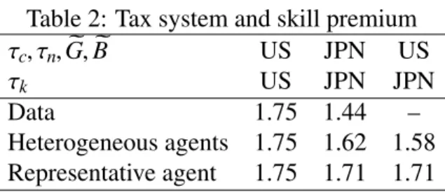
Changes in skill premium Table 2 shows how the skill wage premium changes when the
U.S. tax system is replaced with the Japanese tax system. Replacing the U.S. tax system with
the Japanese tax system means raising the size of the tax and transfer system. By doing so,
the skill wage premium declines by 13 percentage points from 1.75 to 1.62, which corresponds
to 42 percent of the actual difference between the United States and Japan. In addition, we
analyze the impact of a change in policy that replaces the U.S. tax rate on capital income with
the Japanese tax rate, while holding other fiscal parameters fixed. The skill wage premium then
declines even more by 17 percentage points from 1.75 to 1.58, which corresponds to 55 percent
of the actual difference between the United States and Japan.
Table 2: Tax system and skill premium
τc, τn,Ge,Be US JPN US
τk US JPN JPN
Data 1.75 1.44 –
Heterogeneous agents 1.75 1.62 1.58 Representative agent 1.75 1.71 1.71
The skill wage premium declines with a rise in the size of the tax and transfer system in the
representative-agent model as well as the heterogeneous-agents model. However, the magnitude
of the decline is much smaller in the representative-agent model than in the
heterogeneous-agents model.
Decomposition of changes in skill premium To deepen our understanding of the mechanism
of the change in the skill wage premium, we decompose changes in the skill wage premium
into the effect on skilled workers and the effect on unskilled workers (equation 15) and into
the price effect and the composition effect (equation 16). The first and second rows of Table
3 report the log point changes, relative to the U.S. tax system, in the average wage of skilled
workers and the average wage of unskilled workers, respectively. When the U.S. tax system
is replaced with the Japanese tax system, the decline in the skill wage premium is completely
explained by a decrease in the average wage of skilled workers. When the U.S. tax rate on
capital income is replaced with the Japanese tax rate, however, 79 percent of the decline in the
skill wage premium is attributable to a decrease in the average wage of skilled workers, while
A rise in the tax rate on capital income causes a reduction in the capital stock, which results in
a decrease in the average wage of skilled workers who are more complementary to capital, but
possibly an increase in the average wage of unskilled workers who are more substitutable with
capital.
Table 3: Decomposition of the impact of taxes and transfers
τc, τn,Ge,Be US→JPN US
τk US→JPN US→JPN Effect on skilled –8.20 (110.0%) –8.06 (79.0%) Effect on unskilled –0.75 (–10.0%) 2.14 (21.0%) Price effect –5.33 (71.5%) –6.28 (61.7%) Composition effect –2.12 (28.5%) –3.91 (38.3%)
The third and fourth rows report the log point changes, relative to the U.S. tax system, in the
skill wage premium due to the price effect and the composition effect, respectively. When the
U.S. tax system is replaced with the Japanese tax system, the price effect accounts for 72 percent
of the decline the skill wage premium, while the composition effect accounts for the remaining
28 percent. When the U.S. tax rate on capital income is replaced with the Japanese tax rate, the
price effect accounts for 62 percent, and the composition effect accounts for the remaining 38
percent. A rise in the tax rate on capital income causes a reduction in the relative demand for
skilled labor and an increase in the relative supply of skilled labor, which we refer to as the price
effect. At the same time, this causes a reduction in the relative average productivity of skilled
labor, which we refer to as the composition effect. The price effect and the composition effect
work in the same direction to reduce the skill wage premium. The price effect is a significant
factor behind the change in the skill wage premium, while the composition effect is also
non-negligible. Below we discuss the price effect and the composition effect in more detail.
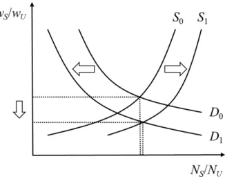
Price and composition effects Figure2illustrates the price effect caused by a rise in the tax
rate on capital income in terms of shifts in the relative supply of and demand for skilled labor. In
the heterogeneous-agent incomplete-markets model, capital income taxation shifts the relative
demand for skilled labor inwards; further, it shifts the relative supply of skilled labor outwards
as a result of the income effect arising from redistribution in the form of capital income taxes
of a change in the interest rate due to a reduction in the capital stock, but such a shift is presumed
to be quantitatively negligible.
Figure 2: The impact of capital income taxation
A change in the composition of workers in the labor market resulting from a rise the tax
rate on capital income alters not only the relative supply of skilled labor but also the relative
average productivity of skilled labor. The shift in the relative supply causes an equilibrium
effect on the skill wage premium, while the change in the relative average productivity causes
a mechanical effect. The willingness to work varies across households according to the market
wage rate and idiosyncratic shocks to productivity in the heterogeneous-agents
incomplete-markets model. Holding other factor fixed, workers are more likely to participate in the labor
market, as the market wage and the productivity shock are higher. When the government raises
the tax rate on capital income and spends the incremental revenue on transfers to households,
unskilled workers are more discouraged to work than skilled workers by the income effect.
Among unskilled workers, the lowest-productivity worker is most likely to exit from the labor
market. The former effect causes the relative supply of skilled workers to shift outwards, thereby
reducing the skill wage premium (Figure2). The latter effect causes the average productivity of
unskilled workers who remain in the labor market to rise, thereby reducing the relative average
productivity of skilled workers, and hence, the skill wage premium. Importantly, both effects
would be even stronger if the government redistributes transfers to unskilled workers more than
to skilled workers. Therefore, the impact of a change in policy that raises the tax rate on capital
Representative vs. heterogeneous agents Given the discussion above, the impact of
capi-tal income taxation on the skill wage premium should be greater in the heterogeneous-agents
incomplete-markets model than in the representative-agent model for two reasons. First, there is
no shift in the relative supply of skilled labor in the representative-agent model (see Appendix
A.2 for details). Consequently, the price effect becomes greater in the heterogeneous-agents
model than in the representative-agent model. Second, there is no composition effect in the
representative-agent model. Since the price effect and the composition effect work in the same
direction in the heterogeneous-agents model, the composition effect leads to an additional
dif-ference in the impact of capital income taxation between the two models.
Changes in other aggregates We validate the model by examining its prediction for the
capital-output ratio and the ratio of the employment rate of skilled workers to that of unskilled
workers. The model predicts that the capital-output ratio is 2.87 under the US tax system, 2.64
under the Japanese tax system, and 2.65 under the Japanese capital income tax rate. The
pre-dicted change in the capital-output ratio is consistent with the data. The capital-output ratio in
Japan was consistently below 2.5 between the years 1995 and 2005 (Hansen and ˙Imrohoro˘glu,
2016), and lower than that in the United States.
The model predicts that the relative employment rate of skilled workers is 1.33 under the
US tax system, 1.19 under the Japanese tax system, and 1.23 under the Japanese capital income
tax rate. The predicted change in the relative employment rate is also consistent with the data.
The relative employment rate in Japan was on average 1.15 in the ESS between the years 1996
and 2006, and lower than that in the United States.
5.3
Welfare implications
We have shown that the skill wage premium significantly declines when the U.S. tax system
is replaced with the Japanese tax system. We now evaluate the impact of such a change in tax
policy on social welfare. To do so, we use the utilitarian social welfare function, as is common
in the literature. We describe the details of the measurement and decomposition of the welfare
Social welfare We consider the impact on social welfare of a change in policy that raises
the U.S. tax rate on capital income to the Japanese tax rate. To measure the welfare effect,
the government consumption-output ratio and the government debt-output ratio are held fixed.
Table 4 shows how the consumption-equivalent welfare changes when the U.S. tax rate on
capital income is replaced with the Japanese tax rate. We find that such a change in tax policy
entails a welfare gain of 1.7 percent in the heterogeneous-agents model. In contrast, it entails a
welfare loss of 0.8 percent in the representative-agents model.
Table 4: Capital income taxation and social welfare
τc, τn,Ge,Be US
τk US→JPN Heterogeneous agents
Welfare 1.73%
Skilled –4.90%
Unskilled 4.54%
Representative agent
Welfare –0.82%
Heterogeneous agents, transition
Welfare 2.74%
Skilled –2.84%
Unskilled 5.08%
The welfare consequences of capital income taxation are completely different in the two
models. Capital income taxation results in distortion, which reduces welfare in the
representative-agent complete-markets model, but improves welfare in the heterogeneous-representative-agents
incomplete-markets model, in which agents tend to work longer and save more than their efficient levels.
While it is desirable to reduce the capital income tax rate to zero in the representative-agent
model, it is desirable to impose some level of taxes on capital income in the
heterogeneous-agents model. Moreover, in the context of a heterogeneous-heterogeneous-agents incomplete-markets model,
government transfers serve as an insurance against idiosyncratic shocks to productivity, as well
as a redistribution to reduce inequality. The distributive impact of taxes and transfers is
particu-larly important in the presence of capital-skill complementarity, because in that case persistent
wage differentials exist between skilled workers and unskilled workers.
We measure social welfare by the weighted sum of lifetime utility of all agents. The second
and unskilled workers. A rise in the tax rate on capital income entails a welfare loss of 4.9
percent for skilled workers but a welfare gain of 4.5 percent for unskilled workers. One reason
for this result is that a rise in the tax rate on capital income results in a reduction in capital
stock, which is undesirable for skilled workers who are more complementary to capital but not
necessarily so for unskilled workers who are more substitutable with capital. In fact, when
the U.S tax rate on capital income is replaced with the Japanese tax rate, the average wage
of unskilled workers increases by 2.1 log points, while the average wage of skilled workers
decreases by 8.1 log points (Table 2). Another reason is that a rise in the tax rate on capital
income is associated with redistribution in the form of transfers. Skilled and wealthier workers
pay more taxes, while unskilled and less productive workers benefit more from transfers.
Decomposition of the welfare effect To deepen our understanding of the mechanism of the
welfare effect, we decompose it into welfare effects attributable to changes in the level and
distribution of consumption and leisure. Table5shows the extent to which the welfare effect is
explained by changes in the level and distribution of consumption and leisure. Capital income
taxation reduces the level of consumption but improves the inequality of consumption and the
level and inequality of leisure. The welfare loss from a reduction in the level of consumption
is greater than the welfare gain from a reduction in the inequality of consumption. The welfare
gain from an increase in the level of leisure is substantially greater than the welfare gain from
the distribution of leisure due in large part to the linearity of leisure in preferences. In total, the
welfare gain from an increase in leisure exceeds the welfare loss from a decline in consumption,
when the U.S. tax rate on capital income is replaced with the Japanese tax rate.
Table 5: Decomposition of the welfare effect
τc, τn,Ge,Be US
τk US→JPN
Welfare 0.73%
Consumption
level –2.71%
distribution 0.44% Leisure
level 2.97%
Welfare along the transition We have so far measured the welfare effect by comparing the
two steady states under different tax systems. This means that the welfare gain or cost in the
transition to the new steady state has been ignored in the measurement. When the two steady
states are compared before and after a rise in the tax rate on capital income, the welfare gain may
be understated because the welfare difference between the two steady states reflects a
substan-tial reduction in the capital stock and the average wage of skilled workers. Along the transition
from the initial steady state to the new steady state, however, the capital stock declines
gradu-ally, and part of the decline in the capital stock results from an increase in consumption. If the
welfare effect is measured after transitional welfare changes are taken into account, the results
may change considerably. The last three rows of Table4report the welfare effect when the
tran-sitional welfare changes for all workers, skilled workers, and unskilled workers, respectively.
We consider a once-and-for-all unexpected change in the capital tax rate. The total welfare gain
resulting from a rise in the tax rate on capital income increases from 1.7 percent to 2.7 percent.
6
Conclusion
We have analyzed the impact of taxes and transfers on the skill wage premium and social welfare
in the context of a heterogeneous-agents incomplete-markets model. We have quantified the
extent to which the skill wage premium declines following a rise in the tax rate on capital income
in the presence of capital-skill complementarity. The analysis indicates that the skill wage
premium declines from 1.75 to 1.62 when the U.S. tax system is replaced with the Japanese tax
system, and to 1.58 when only the U.S. tax rate on capital income is replaced with the Japanese
tax rate. We have further shown that social welfare can effectively improve as a consequence of
such a change in tax policy that reduces persistent wage differentials between skilled workers
References
AIYAGARI, S. R. (1994): “Uninsured Idiosyncratic Risk and Aggregate Saving,” Quarterly Journal of Economics, 109(3), 659–684.
(1995): “Optimal Capital Income Taxation with Incomplete Markets, Borrowing
Con-straints, and Constant Discounting,”Journal of Political Economy, 103(6), 1158–1175.
AIYAGARI, S. R.,ANDE. R. MCGRATTAN(1998): “The Optimum Quantity of Debt,”Journal of Monetary Economics, 42(3), 447–469.
ALONSO-ORTIZ, J., AND R. ROGERSON (2010): “Taxes, Transfers and Employment in an
Incomplete Markets Model,”Journal of Monetary Economics, 57(8), 949–958.
CHANG, Y.,ANDS.-B. KIM(2007): “Heterogeneity and Aggregation: Implications for
Labor-Market Fluctuations,”American Economic Review, 97(5), 1939–1956.
DINARDO, J., N. M. FORTIN, AND T. LEMIEUX (1996): “Labor Market Institutions and
the Distribution of Wages, 1973–1992: A Semiparametric Approach,”Econometrica, 84(5),
1001–1044.
FLODÉN, M. (2001): “The Effectiveness of Government Debt and Transfers as Insurance,”
Journal of Monetary Economics, 48(1), 81–108.
FLODÉN, M., AND J. LINDÉ(2001): “Idiosyncratic Risk in the United States and Sweden: Is
There a Role for Government Insurance?,”Review of Economic Dynamics, 4(2), 406–437.
GUNJI, H., AND K. MIYAZAKI (2011): “Estimates of Average Marginal Tax Rates on Factor
Incomes in Japan,”Journal of the Japanese and International Economies, 25(2), 81–106.
HANSEN, G.,ANDS. ˙IMROHORO ˘GLU(2016): “Fiscal Reform and Government Debt in Japan:
A Neoclassical Perspective,”Review of Economic Dynamics, 21, 201–224.
HEATHCOTE, J., F. PERRI, ANDG. L. VIOLANTE(2010): “Unequal We Stand: An Empirical
HUGGETT, M. (1993): “The Risk-free Rate in Heterogeneous-agent Incomplete-insurance
Economies,”Journal of Economic Dynamics and Control, 17(5–6), 953–969.
KATZ, L. F., G. W. LOVEMAN, AND D. G. BLANCHFLOWER (1995): “A Comparison of
Changes in the Structure of Wages in Four OECD Countries,” inDifferences and Changes in Wage Structures, ed. by R. B. Freeman,andL. F. Katz. University of Chicago Press.
KRUEGER, D.,ANDA. LUDWIG(2016): “On the Optimal Provision of Social Insurance:
Pro-gressive Taxation versus Education Subsidies in General Equilibrium,”Journal of Monetary Economics, 77(C), 72–98.
KRUEGER, D., F. PERRI, L. PISTAFERRI, AND G. L. VIOLANTE (2010): “Cross Sectional
Facts for Macroeconomists,”Review of Economic Dynamics, 13(1), 1–14.
KRUSELL, P., L. E. OHANIAN, J.-V. RIOS-RULL, AND G. L. VIOLANTE (2000):
“Capital-Skill Complementarity and Inequality: A Macroeconomic Analysis,” Econometrica, 68(5),
1029–1053.
LISE, J., N. SUDO, M. SUZUKI, K. YAMADA, AND T. YAMADA (2014): “Wage, Income
and Consumption Inequality in Japan, 1981–2008: from Boom to Lost Decades,”Review of Economic Dynamics, 17(4), 582–612.
NAKAJIMA, T., AND S. TAKAHASHI (2016): “Consumption Taxes and Divisibility of Labor
under Incomplete Markets,” KIER Discussion Paper No. 933.
NUTAHARA, K. (2015): “Laffer Curves in Japan,”Journal of the Japanese and International Economies, 36(C), 56–72.
OECD (2015): Education at a Glance 2015: OECD Indicators. OECD Publishing.
PRESCOTT, E. C. (2004): “Why Do Americans Work So Much More than Europeans?,” Fed-eral Reserve Bank of Minneapolis Quarterly Review, 28(1), 2–13.
TAUCHEN, G. (1986): “Finite State Markov-chain Approximations to Univariate and Vector
Autoregressions,”Economics Letters, 20(2), 177–181.
A
Appendix
A.1
Skill-specific productivity process
We consider the extended version of the heterogeneous-agents incomplete-markets model, in
which the productivity process, as well as the degree of substitution for capital, differ between
skilled workers and unskilled workers. We allow both persistence in productivity ̺j and the variance of idiosyncratic shocks to productivity ςj to differ between skilled workers and un-skilled workers. Following Krueger and Ludwig (2016), we consider a skill-specific
produc-tivity process, in which the persistence is 4.4 percent higher for skilled workers than for
un-skilled workers, while the variance is 92 percent higher for unun-skilled workers than for un-skilled
workers. We eventually set at ̺S, ςS2 =(0.9652,0.1656) for skilled workers and ̺U, ςU2 =
(0.9244,0.2295)for unskilled workers such that the weighted averages of the respective
param-eters remain the same. We then recalibrate a set of paramparam-eters(β, λ, µ, ψS, ψU)to match the same targets as in the analysis above.
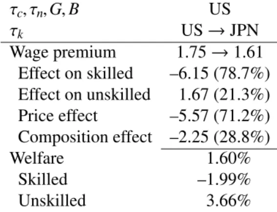
Table6shows changes in the skill wage premium and social welfare in the steady state when
the U.S. tax rate on capital income is replaced with the Japanese tax rate. We confirm that the
main results remain essentially unchanged.
Table 6: Capital income taxation, skill premium, and welfare in the extended model
τc, τn,Ge,Be US
τk US→JPN Wage premium 1.75→1.61
Effect on skilled –6.15 (78.7%) Effect on unskilled 1.67 (21.3%) Price effect –5.57 (71.2%) Composition effect –2.25 (28.8%)
Welfare 1.60%
Skilled –1.99%
Unskilled 3.66%
A.2
Representative-agent model
A.2.1 Households
The economy is populated by a continuum of infinitely-lived households. Each household is
composed of a unit mass of household members who are either skilled or unskilled indexed
by j ∈ {S,U}, and whose preferences are described byUj Cjt,Hjt
, whereCjt is consumption and Hjt is hours worked in period t. We denote sas the share of household members who are skilled.
We consider a problem in which the representative household maximizes the discounted
weighted sum of utility:
∞
Õ
t=τ
βt−τ[sUS(CSt,HSt)+(1−s)UU(CUt,HUt)] (17)
subject to the budget constraint:
(1+τc) [sCSt+(1−s)CUt]=(1−τn) [swStHSt+(1−s)wUtHUt]
+[1+(1−τk)rt]At−At+1+Ft. (18)
Assets Atconsist of physical capital and government debt. We specify the instantaneous utility function to be:
Uj Cjt,Hjt
=lnCjt−ψ
H1+θ
jt
1+θ for j ∈ {S,U}, (19)
where the parameterψ represents the disutility of work, and the parameterθ≥0represents the
Frisch labor supply elasticity.
Utility maximization entails equating the relative prices with the marginal rates of
substitu-tion across goods and time:
CSt=CUt≡Ct, (20)
wSt
wUt =
HSt
HUt θ
, (21)
1+(1−τk)rt=
1
β
Ct+1
Ct
. (22)
conditions (20)–(22), while the capital income tax rate τk appears in the intertemporal opti-mality condition (22). Consumption and labor income taxation influences neither the relative
consumption nor the relative labor supply of skilled labor, while capital income taxation
influ-ences asset holdings.
A.2.2 Firms
Perfectly competitive firms produce output according to the technology (8).
A.2.3 Government
The government levies proportional taxes on consumption, labor income, and capital income,
and spends the tax revenue on government consumption, lump-sum transfers, and interest
pay-ments on government debt, according to the balanced budget rule (13).
A.2.4 Equilibrium
The equilibrium of the economy is characterized as follows. Given policiesnGet,Bet, τc, τn, τk,Fet o
and an initial conditionz0, a competitive equilibrium is an allocation n
e
CSt,CeUt,HSt,HUt,NSt,NUt,KeEt,KeSt o
and price system{weSt,weUt,rt}such that: for allt, given prices, the allocation solves the house-hold’s problem and the firm’s problem; the government budget is balanced; the capital market
clears, i.e.,KeEt+KeSt+Bet= Aet; labor markets clear, i.e., NSt=sHSt andNUt =(1−s)HUt; and the final goods market clears, i.e.,Cet+KeE,t+1+KeS,t+1=F
NSt,NUt,KeEt,KeSt;zt
+(1−δE)KeEt+
(1−δS)KeSt.
A.2.5 Skill premium
The equilibrium skill wage premium is defined as:
ωra≡ wS wU =
1−s s
NS
NU θ
. (23)
The skill wage premium decreases with a rise in the share of the skilled population and increases
same share of the skilled population but different tax systems, the difference in the skill wage
premium is:
∆ln(ωra)=θ∆ln
NS
NU
. (24)
The cross-country difference in the skill wage premium is proportional to the difference in the
relative demand for skilled labor resulting from differences in the tax system.
A.3
Numerical algorithm
We describe methods for computing the equilibria in the heterogeneous-agents
incomplete-markets model.
Steady state We compute the steady-state equilibrium allocation in the heterogeneous-agents
incomplete-markets model by extending the numerical algorithm in Aiyagari and McGrattan
(1998) and Flodén and Lindé (2001), who build upon the algorithm of Huggett (1993) and
Aiyagari(1995).
1. Discretize the state space (ea,x,j), and compute the transition probability π(x′|x) using
theTauchen(1986) method.
2. Set a guess for nKeE,NS,ez o
. ComputeKeSfrom (11) and (12). 3. GivennKeE,KeS,NS,ez
o
, computeweSfrom (9),r from (11),NU from (8),weU from (10), and aggregate consumptionCefrom the goods market clearing condition. Given
n e
G,Be, τc, τn, τk o
,
computeFefrom (13).
4. Solve for the beginning-of-period value functionV(ea,x,j).
(a) Set a guess forV(ea,x,j).
(b) Update the value function using the Bellman equations (5) and (6) until convergence.
Given the value function, obtain the decision rules{ec(ea,x,j),h(ea,x,j),ea′(ea,x,j)}.
5. Compute the stationary distributionξ(ea,x,j).
(b) Update the distribution by weighting the transition probability according to the
dis-tance from the optimal asset holdings to the two adjacent grid points, until
conver-gence.
6. UpdatenKeE,NS,ez o
. Repeat steps 2 to 5 until convergence.
Transitional dynamics We compute the transition path from the initial steady state to the
new steady state as follows:
1. Compute the initial steady state. Assume that the economy converges to the new steady
state after 100 periods, and compute the new steady state.
2. Set a guess for the transition path of nKeEt,KeSt,NSt,ezt o100
t=0
. Given this path, compute the
transition path ofnweSt,weUt,rt,NUt,Cet,Fet o100
t=0.
3. Solve the agent’s problem backwards from the last period to the first period, and obtain
the decision rules.
4. Given the decision rules, simulate the economy forward from the first period to the last
period.
5. UpdatenKeEt,KeSt,NSt,ezt o100
t=0. Repeat steps 2 to 5 until convergence.
A.4
Welfare measurement
We describe the measurement and decomposition of the welfare effect of a change in policy.
Social welfare Social welfare can be defined as the weighted sum of the lifetime utility of all
agents, which depends on consumptioncjand leisure, defined asℓj=1−hj:
Υm ≡
∫
{j=S,U}
Vm(ea,x,j)dξm+
lnY0m
1−β +
βln(1+g)
(1−β)2 (25)
= ∫
{j=S,U}
(
E0
∞
Õ
t=0
βtlnecm−ψj(1−ℓm) )
dξm+
lnY0m
1−β +
βln(1+g)
wherem=0andm=1represent the pre-reform steady state and the post-reform steady state, respectively, andY0 is the initial output. The welfare consequence of a change in the tax rate
can be expressed as the percentage change in consumption, denoted by̟, required to leave the
agents indifferent between the two equilibrium allocations:
∫
{j=S,U}
(
E0
∞
Õ
t=0
βt
h
ln
(1+̟)ec0
−ψj
1−ℓ0
i)
dξ0+
lnY00
1−β
= ∫
{j=S,U}
(
E0
∞
Õ
t=0
βthlnec1−ψj
1−ℓ1i
)
dξ1+
lnY01
1−β. (26)
The welfare effect of a policy reform can then be measured by:
̟=exp[(1−β) (Υ1−Υ0)] −1. (27)
The welfare effect can be decomposed into the portion attributable to a change in consumption
and the portion attributable to a change in leisure. Each of the two effects can be further
de-composed into the portion attributable to a change in the level of consumption or leisure and
the portion attributable to a change in the distribution of consumption or leisure:
1+̟=(1+̟c) (1+̟ℓ)=
1+̟clevel 1+̟cdist 1+̟ℓlevel 1+̟
dist
ℓ
(28)
Or approximately, ̟ ≃ ̟clevel+̟cdist+̟ℓlevel+̟
dist
ℓ . Below we describe the details of the
welfare decomposition.
Decomposition of the welfare effect We decompose the welfare effect into the portion
at-tributable to a change in consumption and the portion atat-tributable to a change in leisure, i.e.,
1+̟= (1+̟c) (1+̟ℓ), and further decompose each of the two effects into the portion
at-tributable to a change in the level of consumption or leisure and the portion atat-tributable to a
change in the distribution of consumption or leisure, i.e., 1+̟c= 1+̟clevel
1+̟cdist
and
1+̟ℓ=
1+̟ℓlevel 1+̟ℓdist
. Given the specification of preferences, it is possible to derive a
closed-form expression for each welfare effect. We first derive1+̟ℓ by the linearity of leisure
then derive 1+̟clevel and1+̟ℓlevel, and calculate 1+̟
dist
c and1+̟ℓdist as the residuals, i.e.,
̟cdist= (1+̟c)/ 1+̟clevel
−1 and̟ℓdist= (1+̟ℓ)/
1+̟ℓlevel
−1. Below we provide the
description ofωℓ,̟ℓlevel, and̟clevel.
We denote Lj as the aggregate leisure of a group j, and define the aggregate leisure as
L= LS+LU. We denote by the superscripts 0 and 1 the pre-reform steady state and the post-reform steady state, respectively. The welfare effect attributable to a change in leisure can be
obtained by changing leisure while holding consumption constant.
̟ℓ =exp h
ψS
LS1−L0S
−ψU
LU1−LU0
i
−1 (29)
The welfare effect attributable to a change in the level of leisure can be described by changing
the level of leisure while holding the distribution and consumption constant.
̟ℓlevel=exp
ψSLS0+ψULU0
L1 L0−1
−1. (30)
Similarly, the welfare effect attributable to a change in the level of consumption can be obtained
by changing the level of consumption while holding the distribution and leisure constant.
̟clevel= C 1