INFORMS is l ocat ed in Maryl and, USA
Management Science
Publ icat ion det ail s, incl uding inst ruct ions f or aut hors and subscript ion inf ormat ion:
ht t p: / / pubsonl ine. inf orms. org
Dynamics of Consumer Adopt ion of Financial Innovat ion:
The Case of ATM Cards
Bot ao Yang, Andrew T. Ching
To cite this article:
Bot ao Yang, Andrew T. Ching (2014) Dynamics of Consumer Adopt ion of Financial Innovat ion: The Case of ATM Cards. Management Science 60(4): 903-922. ht t ps: / / doi. org/ 10. 1287/ mnsc. 2013. 1792
Full terms and conditions of use: http:/ / pubsonline. informs. org/ page/ terms-and-conditions
This ar t icle m ay be used only for t he pur poses of r esear ch, t eaching, and/ or pr ivat e st udy. Com m er cial use or syst em at ic dow nloading ( by r obot s or ot her aut om at ic pr ocesses) is pr ohibit ed w it hout explicit Publisher appr oval, unless ot her w ise not ed. For m or e infor m at ion, cont act per m issions@infor m s.or g.
The Publisher does not war rant or guarant ee t he ar t icle’s accuracy, com plet eness, m er chant abilit y, fit ness for a par t icular pur pose, or non- infr ingem ent . Descr ipt ions of, or r efer ences t o, pr oduct s or publicat ions, or inclusion of an adver t isem ent in t his ar t icle, neit her const it ut es nor im plies a guarant ee, endor sem ent , or suppor t of claim s m ade of t hat pr oduct , publicat ion, or ser vice.
Copyr ight © 2014, I NFORMS
Please scroll down for article—it is on subsequent pages
INFORMS is t he l argest prof essional societ y in t he worl d f or prof essional s in t he f iel ds of operat ions research, management science, and anal yt ics.
ISSN 0025-1909 (print)ISSN 1526-5501 (online) http://dx.doi.org/10.1287/mnsc.2013.1792 © 2014 INFORMS
Dynamics of Consumer Adoption of Financial
Innovation: The Case of ATM Cards
Botao Yang
Marshall School of Business, University of Southern California, Los Angeles, California 90089, [email protected]
Andrew T. Ching
Rotman School of Management, University of Toronto, Toronto, Ontario M5S 3E6, Canada, [email protected]
W
e develop a structural consumer life-cycle model to investigate consumers’ adoption and usage decisionsof ATM cards. If consumers are forward-looking with a known discount factor, our framework can control for the heterogeneous life span faced by consumers of different ages, and hence measure adoption costs more accurately. Moreover, our framework can recover the monetary value of total adoption costs. To estimate our model, we use an Italian panel data set, which contains information on consumers’ adoption decisions for ATM cards, and their cash withdrawal patterns before and after adoption. Our results suggest that one could signifi-cantly overestimate adoption costs for the elderly when ignoring their shorter life span. Our policy experiments show that a sign-up bonus targeted to the elderly could be much more effective if implemented as a limited-time offer rather than a permanent offer. Interestingly, if the sign-up bonus is permanent, younger consumers may strategically postpone adoption.
Keywords: financial innovation; adoption costs; ATM cards; cash demand model; consumer life-cycle model; limited time promotional offer; permanent promotional offer; dynamic programming
History: Received July 16, 2010; accepted June 20, 2013, by Pradeep Chintagunta, marketing. Published online inArticles in AdvanceNovember 13, 2013.
1.
Introduction
The adoption of financial innovation1 has been an important part of household finance in the past forty years. For instance, by adopting new financial instru-ments like ATM cards, credit or debit cards, con-sumers can manage their transaction balances more efficiently. ATMs have significantly reduced the trans-action cost of withdrawing cash from a bank account; credit/debit cards have significantly reduced the need to carry cash for daily transactions. If consumers adopt these financial innovations, they can invest more in an interest-bearing asset and reduce the cost of infla-tion. This in turn can influence the aggregate demand for money and the social costs of inflation. Although this important implication is well recognized and doc-umented (e.g., Attanasio et al. 2002, Alvarez and Lippi 2009), the literature seldom investigates consumers’ adoption decisions of financial innovations. Papers that investigate this issue typically use a reduced-form approach to identify the determinants of adop-tion decisions. These papers have generated many
1Financial innovation is a broadly defined term. In addition to
innovations related to new technologies that reduce transaction costs, the term commonly refers to new types of securities. Tufano (2003) provides an excellent survey of this literature.
useful insights, but they also suffer from one poten-tial limitation: they do not consider the possibility that consumers can be forward-looking and take the future flow of benefits of adopting the new technol-ogy into account. The estimated costs of adopting a new technology can be very different depending on how consumers consider future benefits. Because of this potential shortcoming, these models may generate misleading predictions about how consumers might change their adoption decisions under new marketing environments or public policies.
In light of these implications, the first objective of this paper is to develop a structural framework to analyze forward-looking consumers’ adoption deci-sions of a financial innovation and estimate their adoption costs. To achieve this goal, we assume con-sumers make their adoption decisions to maximize their total discounted future utility; we formulate the problem using dynamic programming. We use our model to study the consumer decision of ATM card adoption, one of the most important financial innovations in the past three decades.2 To estimate
2Paul Volcker, a former chairman of the Federal Reserve,
com-mented in theWall Street Journal’s (2009) Future of Finance Initiative that the ATM was the peak of financial innovation.
903
our model, we use a unique microlevel data set from the Bank of Italy. In addition to demographic charac-teristics and ATM card adoption decisions, the data contain detailed information about cash management decisions at the household level. Such information allows us to model how consumers manage cash before and after adopting ATM cards and impute the per period monetary benefits of adopting the innova-tion even if consumers choose not to adopt in a given period. This allows us to recover the monetary value of total adoption costs.
The Bank of Italy’s unique data set, together with our model, also allows us to shed new light on a stylized fact of technology adoption behavior: Adop-tion rates of many new technologies (e.g., calculators, computers, video recorders, and ATMs) by the elderly are consistently much lower than those by younger age groups (e.g., Kerschner and Chelsvig 1984, Gilly and Zeithaml 1985). Previous literature tries to ratio-nalize this fact by arguing that either the elderly have psychological resistance toward new technolo-gies (technophobia), or that it is relatively difficult for them to learn how to use new technologies (e.g., Adams and Thieben 1991, Hatta and Liyama 1991, Rogers et al. 1996). However, one potential expla-nation has been neglected: the elderly have a much shorter remaining life span than the young, and con-sequently their total discounted benefits from adop-tion could also be much smaller. Ignoring differences in total discounted benefits from adopting a new tech-nology could lead to biased estimates in adoption costs for different age groups and misleading policy implications.
To address this potential problem, the second objec-tive of this research is to show how to use our frame-work to quantify the costs of adopting ATM cards by age. If we assume that consumers understand how age affects longevity, and that their discount factor (from future benefits of an ATM card) is known, we can use our structural model to control for hetero-geneous expected discounted benefits from adoption, and hence measure adoption costs more accurately.3 To illustrate what our model can accomplish, we fix the discount factor to a value (which is 0.943) calcu-lated from consumers’ responses to a survey question
3One important limitation of this research needs to be highlighted. Unfortunately, like most empirical applications of dynamic pro-gramming models, our model does not have exclusion restrictions that can help identify consumers’ discount factor (Magnac and Thesmar 2002, Fang and Wang 2012). Because of this limitation, we need to assume a discount factor; we do not attempt to test whether reduced adoption rates with age are attributable to higher adoption costs or shorter remaining life horizon. To achieve such identification, one needs to first carry out additional research to measure how consumers discount the future benefits generated by the new technology of interest.
on when to cash a lottery, and estimate the rest of the parameters. For this discount factor, we find that total adoption costs remain relatively constant for people over age 50. However, if we assume consumers are myopic (i.e., discount factor=0), estimated adoption costs would increase with age for people over age 50. Our results suggest that if consumers are forward-looking, ignoring this could lead to serious bias in the estimates of adoption costs.
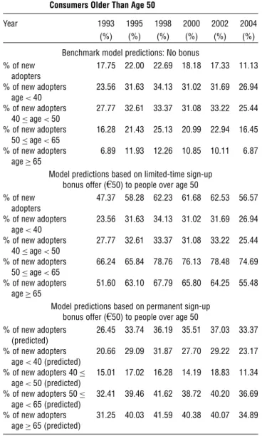
The third research objective is to use our model to study the impact of a sign-up bonus that targets the elderly. It is common for companies to use a sign-up bonus to encourage consumer adoption of new tech-nologies. To shed light on this promotion strategy, we conduct counterfactual experiments where banks give consumers who are age 50 and older a sign-up bonus for adopting ATM cards. We consider two ways to implement the sign-up bonus: (i) limited-time offer, and (ii) permanent offer (i.e., an offer with no expira-tion date). We argue that the limited-time offer would not change consumer expectations about future adop-tion costs, but the permanent offer would. Using our model, we show that these two marketing promotion strategies can lead to dramatically different outcomes: (1) the limited-time offer is much more effective in increasing adoption rates in the older group of con-sumers; (2) adoption rates for consumers who are younger than age 50 drop under the permanent offer. This is because the permanent offer creates an option value for consumers to postpone adopting. In partic-ular, the permanent offer gives younger consumers an incentive to delay adopting ATM cards until they reach age 50. Our counterfactual experiments sug-gest that if consumers are forward-looking, ignoring their strategic delay behavior may cause banks to mis-calculate net benefits of their marketing promotion campaigns.
To the best of our knowledge, this is the first dynamic structural model of technology adoption that (i) provides a framework that could potentially con-trol for consumers’ heterogeneous life horizon when measuring their adoption costs over their life cycle, (ii) models usage decisions of old and new tech-nologies, and (iii) investigates the impacts of two ways of implementing a sign-up bonus to a particu-lar age group: limited-time offer and permanent offer. Although the model appears to be tailored for ATM card adoption, with suitable modifications one can still apply our basic framework to study consumer adoption decisions of other financial innovations such as credit cards, debit cards, or other new payment instruments.
The remainder of this paper is structured as fol-lows. Related literature is discussed in §2. Section 3 outlines relevant institutional details about ATMs and the banking system in Italy. Section 4 describes the
microlevel panel data used in the estimation. Section 5 presents the model. The estimation algorithm, iden-tification issues, and results are discussed in §6. Sec-tion 7 presents the conclusions.
2.
Literature Review
2.1. Adoption of Financial Innovations
Here we study consumers’ adoption decisions of financial innovations that reduce transaction costs for an individual’s cash management. These financial innovations include ATMs (e.g., Attanasio et al. 2002, Huynh 2007), credit/debit cards (e.g., Borzekowski et al. 2008), online banking (e.g., Bauer and Hein 2006), and the automated clearing house (ACH) electronic payment system (e.g., Gowrisankaran and Stavins 2004, Ackerberg and Gowrisankaran 2006), etc. Among these papers, the paper by Bauer and Hein (2006) is more closely related to ours. They investigate whether risk aversion is a determining fac-tor in consumers’ adoption of online banking. They find evidence that this factor plays a key role in younger consumers’ adoption decisions, but is not statistically significant in explaining older consumers’ adoption behavior. Our research complements theirs by showing that shorter remaining life spans can be a plausible explanation for why older consumers are hesitant to adopt.4
Note that all of the above-mentioned papers use the static reduced-form approach to study consumer adoption decisions. They do not explicitly consider consumer expectations about future benefits gener-ated by new technology. Therefore, it is difficult to perform certain policy experiments (e.g., limited-time offer versus permanent offer) based on their estima-tion results. Because our dynamic structural model explicitly takes consumers’ forward-looking behavior into account, it is better suited for policy experiments that will change consumers’ expectations about the future.
2.2. Dynamic Adoption Decision Models
There are several studies in marketing that also use the discrete choice dynamic programming framework and individual level data to study consumers’ tech-nology adoption decisions (e.g., Sriram et al. 2010, Ryan and Tucker 2012).5Unlike our modeling frame-work, their frameworks cannot recover the monetary value of total adoption costs; hence, they are less
4The importance of ATMs has also attracted researchers to examine banks’ ATM adoption decisions (e.g., Hannan and McDowell 1984, 1987; Saloner and Shepard 1995; Ishii 2007; Ferrari et al. 2010). 5Another line of literature uses aggregate level data to study adop-tion decisions of durable goods (e.g., Gordon 2009, Gowrisankaran and Rysman 2012, Nair 2007, Song and Chintagunta 2003), and experienced goods (e.g., Ching 2010a, Chen et al. 2013).
suitable for evaluating the impact of giving a specific amount of a sign-up bonus (or other monetary incen-tives) on adoption decisions.
Another main difference between our model and those in the existing literature is that we use a life-cycle model where consumers face a finite hori-zon, while the papers discussed above use an infi-nite horizon model.6 Our consumer life-cycle model helps us improve the current understanding of adop-tion decisions for different age groups, an area that has been understudied in the previous literature. If we combine our model with other methods to cal-ibrate consumers’ discount factors, we could inves-tigate whether the shorter life horizon faced by the elderly could be a plausible explanation for why they are reluctant to adopt new technologies.7
More broadly, the model is related to the health investment literature (e.g., Fang et al. 2007, Khwaja 2010). Their main point is that, from a dynamic perspective, better insurance may increase one’s life expectancy, and consequently enhance one’s incentive to invest in health. This dynamic effect counteracts the usual “moral hazard” story in static models that insurance induces more risky behavior. We share the idea that the longer the expected planning horizon (life span in our cases), the greater the incentive to invest in the improvement of one’s welfare in the future. Ratchford (2001) also argues that as con-sumers become older, the return to new investments in knowledge becomes smaller. Yet Ratchford (2001) does not investigate this hypothesis empirically.
3.
ATM/Banking System in Italy
ATMs were first introduced to Italy in the 1970s (Canato and Corrocher 2004). Bancomat, the Italian interbanking cash dispenser project, was promoted by the Italian Society for Interbanking Automation start-ing in 1983 (Orlandi 1989). Durstart-ing the time period studied in this paper, Bancomat was the only ATM network in Italy that allowed customers of all Italian banks to use any ATM in the network.8 Many Italian
6Strictly speaking, every consumer should face a finite horizon
problem as they cannot live forever. But an infinite horizon model could be a good proxy when the length of a period is short (e.g., day or week). Here an infinite horizon model would not be a good approximation because the length of a period in our data is two years. This modeling choice is driven by the slow diffusion of ATM cards, and the fact that our main data source is from a biannual sur-vey. Note also that it is common for structural econometricians who study consumer life-cycle decisions to use a finite horizon dynamic programming framework (see, e.g., Keane et al. 2011).
7This hypothesis is also mentioned in Swanson et al. (1997). Their focus is different from ours. Instead of estimating adoption costs, their goal is to understand how consumer adoption of new tech-nologies affects economic growth using a theoretical model. Con-sequently, the details of their model are very different from ours.
8For a more detailed discussion about the evolution of ATMs and
branches in Italy, see Hester et al. (2001).
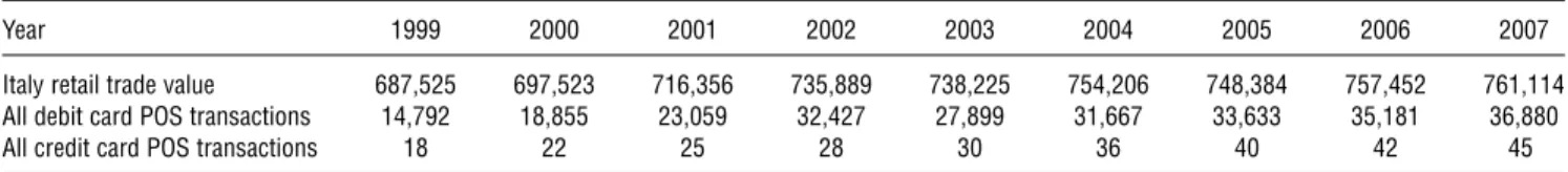
Table 1 Retail Trade, Debit Card Transactions, and Credit Card Transactions (Million Euros)
Year 1999 2000 2001 2002 2003 2004 2005 2006 2007
Italy retail trade value 687,525 697,523 716,356 735,889 738,225 754,206 748,384 757,452 761,114
All debit card POS transactions 14,792 18,855 23,059 32,427 27,899 31,667 33,633 35,181 36,880
All credit card POS transactions 18 22 25 28 30 36 40 42 45
Sources. Italian Institute of Statistics and Bank of Italy.
banks charge a small annual service fee for ATM cards. According to Attanasio et al. (2002), the aver-age annual fee was E6.2 (1995 base) on a sample
of 38 banks. There are no additional service charges when a customer uses an ATM owned by the bank which issues the ATM card. The normal bank account for day-to-day transactions in Italy is a checking account, which also serves as a savings account. Note that all checking accounts in Italy are interest bear-ing, and interest is received quarterly. An ATM card needs to be linked to a checking account before it can be used to withdraw cash. In Italy, banks are usu-ally open from 08:30 to 16:00, with a one-hour break between 13:30 and 14:30; they are generally closed on weekends and holidays. On the day before a holiday, banks are often closed in the afternoon as well. Their restricted hours suggest that ATM cards could signif-icantly reduce the transaction costs of withdrawing cash for many consumers.
Most ATM cards in Italy have the point of sale (POS) functionality, which means they can be used as debit cards at places like shopping malls and super-markets, as long as merchants are equipped with POS terminals to process debit transactions. Table 1 shows the Italy retail trade value, debit card POS transac-tions and credit card POS transactransac-tions from 1999 to 2007. The proportion of retail trade sales paid by debit cards is very small. For example, in 2004, the total retail trade value in Italy wasE754,206 million, while
the debit card POS transactions wereE31,677 million,
accounting for 4.2% of the total retail trade. Even if we take into account that only ATM card holders can make debit card payments at POS terminals, the percentage remains small.9 The values of credit card transactions are even smaller than those of debit card transactions.
The above evidence indicates that consumers in Italy seldom use the POS function of ATM cards. Moreover, credit card payments were uncommon in Italy for the period studied in this paper, i.e., 1991–2004 (Rolfe 2005). This is consistent with a recent comment by Lyman (2009), “Italy, for the most part, remains a cash economy.” These institutional details are important when we implement our cash demand
9The ATM card adoption rate was 57.8% in 2004. If we suppose
that 57.8% of the total retail trade sales came from those adopters in 2004, the percentage becomes 311667/47541206∗005785=703%.
model in §6. They explain why we use consump-tion of nondurable goods as a proxy for consumpconsump-tion financed by cash.
4.
Data
The data used in this paper combine four different data sets: (i) Survey of Household Income and Wealth, (ii) interest rate data at the regional level, (iii) num-ber of ATMs at the provincial level, and (iv) popula-tion and survival probability data. The informapopula-tion in items (i)–(iii) is obtained from the Bank of Italy; data in item (iv) is obtained from the Italian Institute of Statistics.
4.1. Bank of Italy’s Survey of Household Income and Wealth (SHIW)
The SHIW is a comprehensive socio-economic sur-vey. This database contains information regarding: (1) individual characteristics and occupational status, (2) sources of household income, and (3) consumption expenditures.
These surveys were conducted annually from 1977 to 1985, and then biannually from 1987 to 1995 and from 1998 to 2004. We selected a panel from 1991 to 2004 as the sample used for estimation; 1991 is the first year that ATM card information appears in the SHIW, and 2004 is the latest year of data that is avail-able to the public. The key questions for this study in the survey include the following:
1. ATM card: “Did you or any other member of your household have an ATM card?”
2. Average amount of withdrawal at an ATM/bank counter: “What was the average amount per with-drawal?”
Although the total number of households in this survey is around 8,000 in each wave, most are not included in our study because they do not satisfy our selection criteria. A household belongs to our sample if (i) anyone in the household has bank accounts; (ii) all are nonadopters of ATM cards in their first observed periods; (iii) we observe which province they live in; (iv) we observe them through 2004; and (v) they do not abandon ATM cards after adoption. We set these criteria for the following rea-sons. Requirement (i) is a necessary condition for a household to apply for ATM cards. Requirement (ii) stems from the focus of this research, i.e., studying
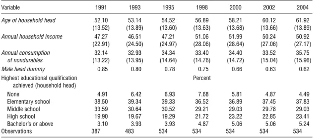
Table 2 Summary Statistics of Main Variables
Variable 1991 1993 1995 1998 2000 2002 2004
Age of household head 52010 53014 54052 56089 58021 60012 61092
4130525 4130895 4130605 4130635 4130685 4130665 4130895
Annual household income 47027 46051 47021 51006 51099 50024 50092
4220915 4240505 4240975 4280065 4280645 4270065 4270175
Annual consumption 32014 32093 34034 33040 34040 33052 35075
of nondurables 4130225 4130955 4140645 4140765 4140725 4150045 4150965
Male head dummy 0085 0080 0078 0075 0066 0063 0062
Highest educational qualification Percent
achieved (household head)
None 4091 6042 6093 7068 5081 4087 4049
Elementary school 38050 39034 39033 36052 36089 37045 37083
Middle school 33059 30064 30052 29021 29003 29078 29003
High school 19090 19067 19029 21072 23022 22085 23041
Bachelor’s or above 3010 3093 3093 4087 5006 5006 5024
Observations 387 483 534 534 534 534 534
Notes. We report means for all key variables except education. Numbers in parentheses are standard deviations, which are not reported for dummy variables. Income and consumption of nondurables are measured in 500 euros (2002).
adoption decisions. We use requirement (iii) because our data on the number of ATMs are broken down at the provincial level. Requirement (iv) ensures that we have a reasonably long panel of households. We set requirement (v) because there are very few house-holds that abandoned ATM cards after adoption. Although a model that allows households to switch back to nonadoption is more general, it will signif-icantly increase the size of the state space for the dynamic programming problem. Moreover, such inci-dences are rare not only for ATM cards, but also for other new technologies. This is shown by the fact that most of the previous research considers the adoption of new technology as an optimal stopping problem (e.g., Ryan and Tucker 2010, Song and Chintagunta 2003, Sriram et al. 2010). We also exclude a few out-liers with relatively high income/consumption lev-els from the panel.10 The total number of households excluded because of (v) or because they are outliers is only 22.
There are 387 households that satisfy these cri-teria in the 1991 survey. In addition, there are 96 and 51 new households in the 1993 and 1995 waves, respectively, that satisfy the criteria and which are included in our sample. Note that there are new households added in each wave of the SHIW, but none of them satisfies requirement (iii) after 1995 because our provincial level residence location data is limited to pre-1998 households.11Altogether, there are 534 households in our sample.
Table 2 shows the summary statistics of some key variables. The sample average age of the household
10We use the cutoffs E75,000 for annual income and E50,000 for
annual consumption.
11Note that the size of one province in Italy is comparable to that of a county in the United States.
head increases from 52 (in 1991) to 62 (in 2004) with standard deviations varied from 13.5 to 13.9. This shows that the data have significant variation in age, and therefore should be suitable for esti-mating a consumer life-cycle model. Both household income and consumption of nondurables show a slightly upward trend. The percentage of male house-hold heads decreases, probably reflecting the demise of male heads and the longer average life span of females. This also indicates that some households may have changed heads over time. Of the total households, 55.62% are in the north or the central area of Italy, and 44.38% are in the south or islands area. The overall educational level of household heads in our sample is quite low in any given year: at most 5.24% hold a bachelor’s degree or above; around 20% have a high school diploma; about 30% have a middle school diploma; almost 40%, the largest segment of the panel population, received an elementary school education; more than 5% received no education at all. Table 3 summarizes the cumulative adoption rate of this panel. Because we only select nonadopters in 1991, the adoption rate is zero in that year. After
Table 3 Cumulative Adoption Rate of ATM Cards (1991–2004, Panel Households Only)
Year 1991 1993 1995 1998 2000 2002 2004
Adoption rate for 0 0.139 0.240 0.436 0.532 0.624 0.665
all panel households
Adoption rate for household 0 0.185 0.297 0.535 0.628 0.717 0.760
head under age 50 in 1991
Adoption rate for household 0 0.044 0.120 0.224 0.270 0.362 0.418
head over age 65 in 1991
Note. ATM card information before 1991 is not included in the Bank of Italy’s public database.
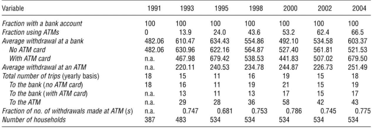
Table 4 Summary Statistics of Cash Withdrawal Behavior
Variable 1991 1993 1995 1998 2000 2002 2004
Fraction with a bank account 100 100 100 100 100 100 100
Fraction using ATMs 0 1309 2400 4306 5302 6204 6605
Average withdrawal at a bank 482.06 610047 634043 554086 492010 534058 603037
No ATM card 482.06 630096 622016 564087 527040 561081 521053
With ATM card n.a. 467098 679042 538053 441083 507002 679050
Average withdrawal at an ATM n.a. 220011 240053 234078 244087 226073 251049
Total number of trips(yearly basis) 18 15 11 16 19 15 18
To the bank(no ATM card) 18 16 11 19 21 15 19
To the bank(with ATM card) n.a. 13 11 13 17 15 17
To the ATM n.a. 29 28 36 58 42 43
Fraction of no. of withdrawals made at ATM(s) n.a. 00747 00681 00753 00786 00745 00775
Number of households 387 483 534 534 534 534 534
Note. Average withdrawals are measured in 2002 euros.
that, the adoption rate increases by about 10% every two years (except for the 20% increase from 1995 to 1998, and the 4% increase from 2002 to 2004). Note that household heads over age 65 have a much lower adoption rate than those under age 50. This is consis-tent with the stylized fact reported in the technology adoption literature (e.g., Gilly and Zeithaml 1985).
Table 4 reports the sample means of some vari-ables of interest that are related to cash management from 1991 to 2004 using our sample. All monetary variables are measured in euros using 2002 as the base year. Table 4 shows that the diffusion of ATM cards is relatively slow among consumers in our sam-ple: It increases from 13.9% (1993) to 66.5% (2004). Note that (i) the average withdrawal at an ATM is much lower than that at a bank counter, and (ii) ATM card adopters make twice as many trips to an ATM compared to the number of trips to a bank for non-adopters. Note also that although ATM card adopters mainly use ATMs to withdraw cash (around 75% of total cash withdrawals), they still withdraw cash from bank counters. Table 5 shows the cash withdrawal behavior within households before and after adopt-ing an ATM card. ATM adopters withdraw a smaller amount of cash on average after adopting an ATM card. These summary statistics provide preliminary
Table 5 Cash Withdrawal Behavior Within Household Before and After Adoption
Variable No. of obs. Mean Std. dev.
Average bank counter withdrawal 283 −10082 684076
before adoption−Average bank counter withdrawal after adoption
Average bank counter withdrawal 288 300004 307024
before adoption−Average ATM withdrawal after adoption
Average bank counter withdrawal 306 191019 360033
before adoption−Weighted average withdrawal after adoption
Note. Average withdrawals are measured in 2002 euros.
evidence that consumers are doing some cost mini-mization based on the withdrawal technology avail-able to them. Because ATMs reduce the transaction time per withdrawal, consumers choose to make more withdrawals and withdraw less cash each time. This allows them to maintain higher average balances in their accounts and hence earn more interest.
Following this argument, consumers with higher consumption of nondurables should benefit more by using ATMs because they need more cash to finance their consumption. Moreover, consumers who have higher income should gain more by adopting ATMs because they have higher opportunity cost of time. Therefore, in terms of adoption behavior, we expect that households with higher consumption of nondurables and higher income are more likely to adopt ATM cards. Our data support this implica-tion. The average annual consumption of nondurables (income) for new adopters is about E3,000–E5,000
(E5,000–E10,000) higher than that of nonadopters.
4.2. Other Data Sources: Interest Rates, Number of ATMs, Survival Probabilities
To control for the opportunity cost of time, we use data on interest rates and ATM density (mea-sured by the number of ATMs per 1,000 popula-tion). The nominal interest rate on current account deposits is drawn from the Bank of Italy’s public database, which is available at http://bip.bancaditalia .it/4972unix/homebipeng.htm. The number of ATMs by province is provided by the Bank of Italy. Note that the interest rate varies across the 20 regions in Italy. Table 6 shows the average interest rate and aver-age ATM density.12The average interest rate increases from 8.9% in 1991 to 10.3% in 1993 and then steadily
12Interest income is subject to a withholding tax in Italy. The with-holding tax rate is 30% before 1997 and 27% since 1998. The flat rate withholding tax is deducted from nominal interest rates in the empirical estimation.
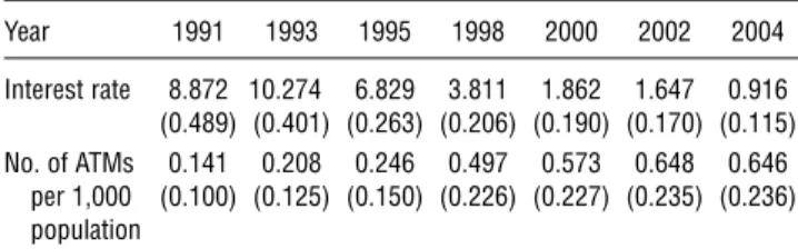
Table 6 Interest Rate and Average Number of ATMs per 1,000 Population
Year 1991 1993 1995 1998 2000 2002 2004
Interest rate 80872 100274 60829 30811 10862 10647 00916
4004895 4004015 4002635 4002065 4001905 4001705 4001155
No. of ATMs 00141 00208 00246 00497 00573 00648 00646
per 1,000 4001005 4001255 4001505 4002265 4002275 4002355 4002365
population
Notes. Numbers in parentheses are standard deviations. There are 20 regions in Italy and interest rate is region-specific. There were more than 90 provinces in Italy between 1991 and 2004; the number of ATMs is province-specific.
decreases to 0.9% in 2004.13 The standard deviation of interest rates decreases from 0.489 in 1991 to 0.115 in 2004, indicating that it differs across regions. The ATM density increases steadily from 0.14 in 1991 to 0.65 in 2002, and then remains at 0.65 in 2004. Note that the standard deviation of the ATM den-sity increases from 0.100 to 0.236, indicating that it becomes more disparate across provinces over time.
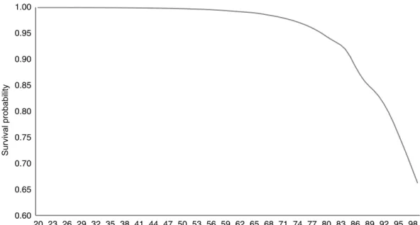
Because we use a life-cycle model to study the data, we use age-specific survival probability to control for the expected life horizon. We obtain the data from the Italian Institute of Statistics (http://demo.istat.it/ index_e.html). Figure 1 shows the 2004 Italian national level survival probability conditional on age (the prob-ability of surviving untilt+1 at aget). It is a decreas-ing and nonlinear function of age.
5.
Model
Before explaining the mathematical model, we briefly discuss the benefits and costs associated with adopt-ing an ATM card. The benefits from adoptadopt-ing an ATM card mainly come from the reduced transaction cost of withdrawing cash, more interest earned (as one can afford to make more withdrawals and put more savings in an interest-bearing bank account on aage), and increased convenience (24-hour ATMs ver-sus daytime human tellers). On the other hand, there are two types of costs involved with adopting an ATM card: (i) monetary costs including ongoing annual and transaction fees, and (ii) nonmonetary costs includ-ing learninclud-ing, hassle, psychological costs, etc. Note that bank customers can use their ATM cards at their own banks for free. Therefore, it seems that to a large extent, consumers can manage to avoid transaction fees. Although we do not observe the amount of annual fees paid by each household, this should not pose a major problem because we are interested in recovering total adoption costs (i.e., monetary plus nonmonetary adoption costs). Next we discuss the model in detail.
13For more details, see the technical appendix of Huynh (2007).
5.1. Adoption Benefits: A Cash Demand Model
To quantitatively measure the cost savings from adopting an ATM card, we use an extension of the Baumol–Tobin cash demand model (Baumol 1952, Tobin 1956).14 It is a cash inventory management model where a consumer chooses the average amount of withdrawal, m, to minimize the sum of transac-tion costs and interest losses,T C.15Interest losses are the forgone interest from holding cash rather than putting it in an interest-bearing bank account (recall that checking accounts are interest-bearing and the highest observed nominal interest rate is 10.3% in 1993). The objective function is shown in the follow-ing equation:
min
m T Cj=w·Tj·
c
j m
+R·
m
2
1 (1)
where j =0 means without ATM cards and j =1 means with ATM cards; w is the unit time cost of transaction (opportunity cost of time); Tj is the trans-action time of each withdrawal given technology j (note that T0> T1); cj is the consumption financed by cash in each time period given technology j, so cj/m is the average number of withdrawals in each period; and R is the interest rate. The first term, w· Tj·4cj/m5, captures the total transaction costs in each period. The second term,R·4m/25, measures interest losses because the average cash inventory in hands is m/2. There is a trade-off between reducing trans-action costs and avoiding interest losses: a larger m means a smaller number of withdrawal transactions, but more interest losses in each period. Simple alge-bra gives us the optimal amount of cash withdrawal and the minimized total cost:
m∗
j =
q
2w·Tj·cj/R=
q 2Tj·
q
w·cj/R1 (2)
T C∗j =q2w·Tj·cj·R=
q 2Tj·
q
w·cj·R0 (3)
The total cost saving from adoption per period can be represented by the difference between the mini-mized total cost without an ATM card (T C∗05 and the minimized total cost with an ATM card (T C∗
15:
ãT C=T C∗
0−T C∗1=4 p
2T0·c0−p2T1·c15·√w·R0 (4)
Section 6.2 discusses how we use household income and consumption of nondurables to approximate w andcj.
14This model is also called the money demand model in the
mon-etary economics literature.
15Alvarez and Lippi (2009) extend the basic Baumol–Tobin model
to a dynamic environment that focuses on precautionary motives.
However, they do not model adoption decisions of ATM cards.
Instead, they study the impact of ATMs on the money demand and welfare costs of inflation, taking ATM card adoption decisions as exogenously given.
Figure 1 Age-Specific Survival Probability in Italy
0.60 0.65 0.70 0.75 0.80 0.85 0.90 0.95 1.00
20 23 26 29 32 35 38 41 44 47 50 53 56 59 62 65 68 71 74 77 80 83 86 89 92 95 98
Age
Su
rvi
va
l
p
ro
b
a
b
ili
ty
5.2. ATM Card Adoption: An Optimal Stopping Problem
Following the previous literature of new technology adoption, we model consumer ATM card adoption decisions as an optimal stopping problem. Letait be the adoption status in period t, where ait=1 if the head of household i chooses to adopt ATM cards; ait=0 otherwise. Note that ait is a choice variable at time t, but it becomes one of the state variables at timet+1.
Let Sit=4ait−11S¯it5 be the vector of state variables for household i at time t. In addition to ait−1, the set of state variables,S¯it, includes year (t), age (ageit5, number of ATMs per 1,000 population (nit), income (yit), consumption of nondurables (cit), interest rate (Rit), age-specific survival probability (zit),16and other household demographic characteristic (Xit). The util-ity function of a potential adopteri (withait−1=0) is assumed to be
Uit4ait3ait−1=01S¯it5
=
(
B4ãT Cit4S¯it51nit5+4t5−Fit+ei1t if ait=11
ei0t if ait=01 (5a)
whereãT Citis the cost saving from adoption defined in the previous subsection;nitis the number of ATMs per 1,000 population;4t5 captures the ATM techno-logical progress over time;17 F
it is the one-time lump
16Note that we treat the survival probability as a function of age only. Therefore, once we includeageit, addingzit to the problem
does not increase the size of the state space.
17For example, ¡4t5/¡t > 0 means the ATM technology has
improved over time; it might become more reliable, secure, or ver-satile (with more functions).
sum adoption cost; and ei0t and ei1t are unobserved independent and identically distributed (i.i.d.) taste shocks. Because only utility difference matters, we normalize the mean utility of waiting (i.e., ait=0) to zero. The utility function of a consumer who has already adopted ATM cards (i.e.,ait−1=15is assumed to be
Uit4ait=13ait−1=11S¯it5=B4ãT Cit4S¯it51nit5+4t50 (5b)
Note that there is no taste shock associated with Uit41311S¯it5because we assume that this is an optimal stopping problem (i.e., once someone adopts, he or she will always keep the ATM card). Also,U 40311S¯it5 does not exist because we assume that adoption is an absorbing state.
Let zit be the survival probability of the head of householdiatageit, and be the discount factor. We assume that in each period, nonadopters chooseaitto maximize their total expected discounted utility. This dynamic adoption decision problem can be formu-lated using dynamic programming. The value func-tion for a potential adopter i (i.e.,ait−1=05 can then be written as
V 4ait−1=01S¯it5
=Eemax8V04ait−1=01S¯it51 V14ait−1=01S¯it591 (6) where Ee is the expectation with respect to the error terms,eijt’s.
A potential adopteri’s alternative-specific value of waiting in timet (i.e.,ait=0) is
V04ait−1=01S¯it5
=U 40301S¯it5+zit+1Z V 4ait=01S¯it+15 dF 4S¯it+1 ¯Sit5
=zit+1 Z
V 4ait=01S¯it+15 dF 4S¯it+1 ¯Sit5+ei0t1 (7)
and his alternative-specific value of adopting an ATM card in timet (ait=15is
V14ait−1=01S¯it5
=U 41301S¯it5+zit+1 Z
V14ait=11S¯it+15 dF 4S¯it+1 ¯Sit5
=B4ãT Cit4S¯it51 nit5+4t5−Fit
+zit+1Z V14ait=11S¯it+15 dF 4S¯it+1 ¯Sit5+ei1t0 (8)
For a household that has already adopted in previous periods, the alternative-specific value of holding an ATM card in timet (ait=15 is
V14ait−1=11S¯it5
=U 41311S¯it5+zit+1 Z
V14ait=11S¯it+15 dF 4S¯it+1 ¯Sit5
=B4ãT Cit4S¯it51 nit5+4t5
+zit+1Z V14ait=11S¯it+15 dF 4S¯it+1 ¯Sit50 (9)
Since we do not allow households to abandon ATM cards, there is no expression forV04ait−1=11S¯it5.
6.
Estimation
We use the nested fixed point algorithm to estimate the structural parameters of the model (Rust 1987). We assume that ifageit>age, thenzit=0. This allows us to use the backward induction approach to solve for the value function.18 Following Rust and Phelan (1997), we setage=102. Note that the oldest observed age in our sample is 97.
6.1. Econometric Specification
6.1.1. Adoption Benefits and Adoption Costs.
We now explain in detail how to measure adoption benefits per period in monetary values. To continue from §5.1, we assume that the opportunity cost of time, wit, is a function of household income, yit, and that the amount of consumption financed by cash, cj1 it, is a function of consumption of nondurables,cit; the cash withdrawal technology is captured by j. In our econometric specification, we use wit=·yit, and cj1 it=j·cit, where and j are constants and 0< j≤1. ATM card holders might make purchases through POS transactions, so a smaller proportion of their consumption is paid by cash. Therefore, we allow06=1, which indicates that the proportion of consumption of nondurables financed by cash is con-ditional on the ATM card adoption status. With these
18Aguirregabiria and Mira (2010) and Keane et al. (2011)
pro-vide excellent recent surveys of the nested fixed point algorithm and other alternative methods to estimate dynamic programming models.
specifications, we definej=q2jTj. It then follows that
m∗
jit=j·
p
yitcit/Rit1 (10)
ãT Cit=40−15· p
yitcitRit0 (11)
We assume that cj1 it is a function ofcit for four rea-sons. First, as discussed in §3, during the period stud-ied in this paper, ATM cards in Italy were mainly used for cash withdrawals. Second, consumption of durables is less than 10% of consumption of non-durables for the households in our sample. Third, around 70% of the observations have zero consump-tion of durables. Fourth, people might use credits to purchase more expensive durable goods. So we believe that (a certain proportion, j, of) consump-tion of nondurables is a reasonable approximaconsump-tion of consumption financed by cash.
However, we cannot directly apply the above equa-tions to the data. One complication is that ATM adopters can withdraw cash from both bank coun-ters and ATMs while nonadopcoun-ters can only do bank counter withdrawals. Table 4 shows that ATM adopters still use bank counters to withdraw cash for around 25% of total withdrawals. To accommodate this feature, we need to modify our cash demand model as follows. Define the share of consumption financed by ATM withdrawals as
sit =value of ATM withdrawals /(value of ATM withdrawals
+value of bank withdrawals)0
We can then rewrite the expression forãT C as
ãT Cit=sit·40−15· q
yitcitRit019 (12)
We further assume that
sit=s+it1 (13)
whereitis an i.i.d. error term with mean zero. To measure ãT Cit, we also need to know 0 and 1. To estimate them, we add an error term to Equation (10),
m∗
jit=j·
p
yitcit/Rit+jit0 (10’)
19An intuitive way to interpret this new equation is to divide total cash spent in each time period into two parts: (i) cash withdrawn from ATMs, and (ii) cash withdrawn from bank counters. ATM adopters have efficiency advantages over nonadopters only for the
first part, which takes up s share of the total cash spent.
Equa-tion (1) then becomes minmT Cj=w·Tj·44s·cj5/m5+s·R·4m/25. We
can easily derive Equation (12) from the optimality condition.
For the expected benefit function,B4ãT Cit1 nit5, we assume that
B4ãT Cit1 nit5
=E6T C·ãT Cit7+n·nit
=E6T C·sit·40−15· q
yitcitRit7+n·nit1 (14)
where T C can be interpreted as the marginal util-ity of income becauseãT Cit is expressed in monetary value.20
Before consumers adopt ATM cards, it is plausible that they know their own 4yit1 cit1 Rit1 nit5. Yet there could be many unforeseen factors that affect sit. As a result, we assume that they do not observesit and hence the expectation above comes down to taking expectation with respect to sit. Then Equation (14) becomes
B4ãT Cit1nit5=T C·s·40−15· q
yitcitRit+n·nit0 (14’)
To capture the technological progress of ATMs, we specify 4t5=∗44t−15/t5. We further specify the adoption cost as
Fit=F0+old·4ageit−50ageit>505+young
·450−min8age9+1ageit>505+young
·4ageit−min8age9+1ageit≤5051 (15)
where min8age9, the minimum observed age of the household head in our sample, is 20.
The above formulation allows the adoption costs to vary with age and the coefficients of age-specific adoption costs to be different in two age groups: old 4young5 is for the over (less than) 50 age group. We choose this functional form because it is relatively convenient to interpret the meanings of these two key coefficients in Equation (15). As for the choice of age=50 as the cutoff, we also tried 60 and 65 as cut-off points in static model estimations. The qualitative results do not change and the goodness-of-fit of these two alternatives is inferior. This suggests that 50 may be a good choice. Note also that Italians usually retire in their fifties (e.g., seeBBC News2007) and people’s cost structure might change (physiologically and psy-chologically) after retirement.
6.1.2. Evolution and Consumer Expectation About State Variables. We assume that nit, yit and cit each follow an independent Markov process. Regarding consumer expectations about the evolution of the state variables, we believe that consumers are generally better at forecasting “internal” variables,
20In the results section, we use
T Cto convert the estimated
adop-tion costs to monetary value.
such as yit and cit, than “external” variables, such as improvements of new technology and interest rates.21 Yet one external variable, n
it, is likely an exception because it can be easily observed and is probably one of the key variables that consumers pay attention to. (This is why we allow nit to enter the utility function directly.) We, therefore, assume that consumers have rational expectations about yit, cit, and nit; i.e., they know the stochastic processes that govern the evolution of these variables. For simplicity, we assume consumers treat Rit and 4t5 as time invariant when solving their dynamic pro-gramming problem.22 Finally, X
it, which includes gender, location, and education, is usually fixed over time, except when the household head changes. In the model, we therefore assume that changes of household head always come as a surprise. Hence, when solving the dynamic programming problem, consumers also treatXitas time invariant.
We specify the stochastic processes of yit, cit, and nit as follows:
nit+1= 00056
(0.005)+(0.010)00986 ∗nit+n1 R
2=009573 (16)
yit+1= 00714
(0.014)∗yit+(0.042)00632 ∗ageit+1
− 000063 (0.0005)∗age
2
it+1+y1 R2=008953 (17)
cit+1= 00693
(0.015)∗cit+(0.028)00468 ∗ageit+1
− 000045 (0.0003)∗age
2
it+1+c123 R2=009160 (18)
Note that theR2’s of these equations range from 0.895 to 0.957, indicating that they are reasonable approxi-mations of the evolution processes.
21By internal variables, we mean consumers have some control
over them (even though we might not model those decisions explic-itly). By external variables, we mean individual consumers do not have control (or have very little control) over them.
22Starting in 1982, the Wall Street Journal conducted polls asking economists for biannual interest rate forecasts and predictions. It was found that not only were these economists not even close in forecasting actual interest rates, they also could not predict the direction in which interest rates would move. In fact, in their fore-casts, experts accurately predicted the direction of interest rates less than one third of the time (Sjuggerud 2005). We view this as evi-dence that it may not be reasonable to assume that consumers can forecast interest rates well. Because it is not clear how consumers form expectations about future interest rates, we assume that they treat it as time invariant in our application for simplicity.
23It is possible that the adoption of ATM cards may increase con-sumption because adopters have easier access to cash. If this effect is important and consumers do anticipate it, one should includeait
in the consumption evolution process. In a robustness check (avail-able upon request), we find that adopting ATM cards increases consumption by 4.66% on average. This would convert to a 2.30%
We discretize nit, yit, and cit into separate grid points. The range ofnitis from 0 to 1.5. We evenly dis-cretize it into 16 points (0100110021 0 0 0 1105). The range of yit (cit) is from 0 to 150 (0 to 100). We evenly dis-cretize yit and cit into 11 grid points; each unit cor-responds to E500. In addition, we discretize R
it into 9 grid points. We also have a time trend4t5, which takes 6 different values corresponding to 6 survey waves from 1993 to 2004. As a result, our state space has 104,544 (=16∗11∗11∗9∗6) grid points.
6.1.3. Likelihood with Unobserved Heterogene-ity: A Concomitant Variable Latent Class Model. Let t0
i be the first observed time period of consumer i, tT
i be the last observed time period of consumer i, and ta
i be the time period that consumer i adopts. Again,ai1 t=0 means consumerichooses not to adopt at time t, and ai1 t=1 means consumer i chooses to adopt at time t. We allow 4j1 s1 n1 F05 to be hetero-geneous, and use the latent class approach to cap-ture it. In other words, we allow 4k
j1 sk1 kn1 F0k5, for
k=11 0 0 0 1 K. Let k be the index for the unobserved type of consumers. Each type has its own set of parameters for the cash demand model and dynamic adoption model. Let Lit4k5 be the individual likeli-hood for type k and k
i be the probability of being typek. Letf 4m∗
jitSit1 k5be the density of observedm∗jit
(m∗
1itis average ATM withdrawal;m∗0itis average bank withdrawal). We assume that the measurement errors in the cash demand model are i.i.d. across time and consumers. Letg4sits1 k5be the density of observed sit (share of ATM withdrawals).
Fort < tai1
Lit4k5=Pr4ait=0 ¯Sit1k5·f 4m∗
0itSit1k50 (19)
Fort=ta i1
Lit4k5=Pr4ait=1 ¯Sit1k5·f 4m∗1itSit1k5g4sits1k50 (20)
Fort > ta i1
Lit4k5=f 4m∗1itSit1k5·g4sits1k50 (21)
We adopt the concomitant variable latent class segmentation approach (Dayton and McReady 1988, Gupta and Chintagunta 1994) and specify the proba-bility that household i belongs to segment k, k
i, as follows:24
k i =
exp401 k+X1 k∗Xi1 t5
1+PK
k=1exp401 k+X1 k∗Xi1 t5
0 (22)
increase in adoption benefits. Therefore, we do not expect that includingaitin the consumption process would have a significant
impact on our results.
24An alternative and more flexible approach is to allow X
i1 t to
enter the utility function directly, and treatk
i’s as parameters to
be estimated. The disadvantage is that it will dramatically increase the computational burden of the estimation algorithm because each value ofXi1 trequires us to solve a different dynamic programming
problem. On the other hand, the concomitant latent class approach
The demographic variables (Xi1 t) include education, gender, and location. Yet on a few occasions, the household head probably changed because the orig-inal household head died. Consequently, Xi could change over time. If the change happened at timet′
i, we allowk
i to be different in the prechange and post-change stages, and the likelihood contribution of Li becomes X k k i · t′ i Y
t=t0
i
Lit4k5
∗
X
k ′k
i · tT
i Y
t=t′ i+1
Lit4k5
0 (23)
For the error terms in the cash withdrawal equa-tions, we assume that ijt∼N 401 2
j5. For the error
term in the share of ATM transactions, we assume that vit∼N 401 2
v5. Also, following Rust (1987), we assume that the unobserved taste shocks in the adop-tion equaadop-tions, ei0t and ei1t, are i.i.d. extreme value distributed. Therefore,
Pr4ait=1 ¯Sit1 k5=Pr4V1k401S¯it5 > V0k401S¯it55
= exp4V¯
k
1401S¯it55 exp4V¯k
0401S¯it55+exp4V¯1k401S¯it55 1
Pr4ait=0 ¯Sit1 k5=Pr4V1k401S¯it5≤V0k401S¯it55
= exp4V¯
k
0401S¯it55 exp4V¯k
0401S¯it55+exp4V¯1k401S¯it55 1
whereV¯k
j401S¯it5=Vjk401S¯it5−eijt,j=011.
6.2. Identification (Intuitive Arguments)
Identification for the cash demand model is rela-tively straightforward. Our data set exhibits large variations in household income and consumption of nondurables as shown in Table 2. Our data also indi-cate significant differences between bank withdrawals and ATM withdrawals as shown in Tables 4 and 5. In addition, there is large time series and some cross-sectional (by region) variation in interest rates as shown in Table 6. These sources of data variation, together with the observed ATM card adoption status of each household and the corresponding withdrawal behavior, allow us to identify the parameters of the cash demand model.
Identification for the adoption costs is less obvi-ous. Initially, it may seem difficult to disentangle the relative importance of the adoption benefits explana-tion and the tradiexplana-tional explanaexplana-tions that emphasize adoption costs. Our hypothesis implies that the total expected discounted benefits of adoption decrease with age; the traditional hypotheses imply that adop-tion costs increase with age. Both approaches can
is not as restrictive as it may seem. Although there are onlyKlatent classes in our model, our approach still allows us to capture the marginal impacts ofXi1 ton adoption decisions via its effects onik.
explain why consumers become more reluctant to adopt as they become older. If all we observe are con-sumer adoption decisions at different ages, it would be impossible to separately measure the relation-ship between costs and age versus the relationrelation-ship between benefits and age. To uncover the relation-ship between adoption costs and age, we also need to (i) assume that the consumer discount factor and the survival probability (which depends determinis-tically on age) are known, so that we can calculate the total discounted benefits of adopting ATM cards;25 and (ii) observe some factors that will shift the adop-tion benefits (i.e., benefit shifters) but not the adopadop-tion costs for any given age.26 In general, the more data variation we have in benefit shifters, the more pre-cisely we can estimate the adoption cost parameters.
In our application, the cash demand model gen-erates the per period adoption benefits over time for each household, which depend on interest rates, household income, and consumption of nondurables. These three variables can be considered benefits shifters. Given our assumption about the discount fac-tor and the age-specific survival probability, we can combine the per period adoption benefits and stochas-tic evolution processes of yit, cit, and nit to compute the total discounted adoption benefits. If individual level data provide variation in benefit shifters Rit, yit, and cit, when we fix an age group, then we can identify the adoption costs for this age group. As shown in the data section, our data set indeed pro-vides variations in these variables. However, to esti-mate adoption costs by age, we will certainly require a very large amount of data to get precise estimates. We therefore opt to use a parsimonious approach by specifying a functional form relationship, as shown in Equation (15). We present more formal identification arguments in Appendix A.27
6.3. Estimation Results
When estimating models with forward-looking agents, researchers typically fix the discount factor according to the interest rate because this parame-ter is usually difficult to identify (Keane et al. 2011). As with most previous work, we will not estimate the discount factor in our maximum likelihood proce-dure. Instead of calibrating it according to the interest
25Note that although the planning horizon is stochastic, it is not estimated. We assume that consumers use the observed survival probability by age (which is publicly available) to set up their plan-ning horizon.
26Strictly speaking, to identify adoption costs, we need to observe mixed adoption decisions. If no one adopts for a given age, even if we observe a range of adoption benefits, we can only identify the lower bound of the adoption costs at that age.
27For a more general discussion about identification for this class of dynamic models, see Arcidiacono and Miller (2013).
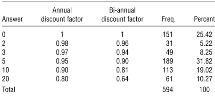
rate, we use the responses to one question asked in SHIW, which aims at soliciting consumers’ time pref-erences. In Appendix B, we show this survey ques-tion and the distribuques-tion of the responses. We set the annual discount factor at the average response to this question, which is 0.943. Note that the discount fac-tor can be context specific. It is unclear whether the discount factor solicited by the survey question neces-sarily applies to ATM card adoption decisions. There-fore, readers should remain cautious when reading our results below.
6.3.1. Which Model Performs the Best? In total, we estimate three specifications based on models with one, two and three latent segments. According to both Akaike information criterion (AIC) and Bayesian information criterion (BIC), the model with two seg-ments produces the best fit.28 Figure 2 shows that the two-segment specification fits the adoption rates over time very well. In terms of goodness-of-fit for the cash demand model, the R-squares are 0.68 and 0.48 for the ATM (868 observations) and bank counter (1,870 observations) withdrawals, respectively. Given that our cash demand model relies only on four parameters to fit the withdrawal patterns, we find the R-squares reasonably satisfactory. Because the two-segment model produces better fit, we will focus our discussion on it and use it to conduct counterfactual experiments.
6.3.2. Parameter Estimates. Table 7 shows the estimation results for the two-segment model. Most of the parameters in the adoption model and cash demand model are statistically significant, except for 1
n. The point estimate of is positive, which sug-gests that consumers care about the technological improvement of ATMs. The point estimate of 2
n is positive, which implies that segment 2 consumers care about the density of ATMs. According to the point estimates, 4k
0−k15 >0. It follows from Equa-tion (11) that consumers can reduce total transacEqua-tion costs of managing cash (i.e., ãT C >05 if they adopt ATM cards. The point estimate of T C is positive, which suggests that ãT C (generated from the cash demand model) is a good measure of adoption bene-fits. One advantage of having a cash demand model is that we can impute the potential adoption ben-efits for consumers who choose not to adopt ATM cards. Table 8 summarizes the monetary values of ãT C over time for adopters and nonadopters, respec-tively. As expected, adopters generally save more than nonadopters by using ATM cards. Finally, because the interest rate starts to decrease after 1993, the average
28The results for one- and three-segment models are available upon request.
Figure 2 Cumulative Adoption Rate: Actual and Predicted
0 0.1 0.2 0.3 0.4 0.5 0.6 0.7 0.8 0.9 1.0
1993 1995 1998 2000 2002 2004
All panel households (actual) All panel households (predicted) Up to 50 years in 1991 (actual) Up to 50 years in 1991 (predicted) More than 65 years in 1991 (actual) More than 65 years in 1991 (predicted)
Year
C
u
mu
la
ti
ve
a
d
o
p
ti
o
n
ra
te
value of ãT C gradually falls from E14.57 (E10.45) in
1993 toE4.18 (E3.00) in 2004 for segment 1 (segment 2)
consumers.
Table 7 Main Estimation Results
=00943, average
self-reported beta Static model
Parameter Estimate S.E. Estimate S.E.
(time trend) 10787∗∗ 00260 60173∗∗ 10083
TC(adoption benefit) 00032∗∗ 00004 00087∗∗ 00011
sk(k=1) 00877∗∗ 00201 00626 00774
k
0(k=1) 50350∗∗ 10382 110020∗∗ 10545
k
1(k=1) 20248∗∗ 00235 50591∗∗ 00349
k
n(no. of ATMs,k=1) −00050 00544 −20122 10804
sk(k=2) 00748∗∗ 00039 00754∗∗ 00038
k
0(k=2) 30248∗∗ 00143 30193∗∗ 00126
k
1(k=2) 00640∗∗ 00023 00661∗∗ 00021
k
n(no. of ATMs,k=2) 00219∗ 00093 00725∗ 00314
F1
0(adoption cost 150551∗∗ 10918 70418∗∗ 00964
in segment 1) log(F2
0−F 1
05(log(adoption −10881∗ 00812 −30251 30579
cost difference))
log( 05 60975∗∗ 00020 60953∗∗ 00022
log( 15 50663∗∗ 00023 50628∗∗ 00024
log(v5 −10233∗∗ 00025 −10230∗∗ 00025
old(age-specific adoption −00012 00010 00065∗∗ 00009
cost, age>50)
young(age-specific adoption −00175∗∗ 00035 00005 00007
cost, age<50)
0 −00352∗∗ 00087 −00425∗∗ 00104
sex −10915 10243 −00663 00793
north −20505 50204 −00571 00929
edu1(none) −20382∗ 00971 −20444∗∗ 00841
edu2(elementary) −00791 20883 10053 10142
edu3(middle school) 10666 10162 10133 10132
−ll 16,268.4 16285.3
N 5,489 5,489
AIC 32,582.8 32,616.6
BIC 32,734.84 32,768.64
∗Significant at 95% confidence level;∗∗significant at 99% confidence level.
Consistent with common wisdom, education is an important predictor for which segment a household belongs to. Household heads with a lower level of education, namely, none or elementary school, are much more likely to belong to the segment with larger adoption costs and smaller adoption benefits. Resi-dency in the north or south does not affect an indi-vidual’s likelihood to fall into a given segment.
6.3.3. How Large Are the Adoption Costs? For identification reasons, we assume that the adoption costs for the second segment are higher than those for the first segment (i.e., F2
0 −F01>0). The estimated total adoption costs in monetary value when age=51 are E166.06 and E168.52 (2002 base) for segment 1
and segment 2, respectively. (We obtain the monetary
Table 8 Consumers’ Cost Savings per Year from Adopting ATM Cards (ãTC)
1991 1993 1995 1998 2000 2002 2004
Segment 1
Mean cost savings 13046 13089 11014 7081 5091 5042 3017
for nonadopters 450805 460005 440895 430595 420685 420475 410545
Mean cost savings n.a. 18076 14075 10091 8022 7080 4069
for adopters 480465 460165 440235 430285 430195 410985
Mean cost savings 13046 14057 12000 9016 7014 6091 4018
for both adopters 450805 460605 450465 440265 430255 430175 420005 and nonadopters
Segment 2
Mean cost savings 9065 9096 7098 5060 4024 3089 2027
for nonadopters 440165 440305 430515 420575 410925 410775 410105
Mean cost savings n.a. 13045 10057 7082 5089 5059 3036
for adopters 460075 440425 430035 420355 420295 410425
Mean cost savings 9065 10045 8060 6057 5012 4095 3000
for both adopters 440165 440735 430915 430065 420335 420275 410435 and nonadopters
Notes. Measured in 2002 euros. Numbers in parentheses are standard deviations.
value by usingT C.) Note that Attanasio et al. (2002) estimate the upper bound of adoption costs to be
E28.1, which is much lower than our estimates. This
is because they assume households only care about the current period benefits of adopting the ATM card instead of its total discounted future benefits.
Our results also allow us to investigate how adop-tion costs vary with age. According to our estimates, elderly people might not have larger adoption costs. Note that the age-specific component of adoption costs for people over age 50, old, is not signifi-cantly different from zero. This indicates that adop-tion costs are fairly flat for people over age 50. This finding is very different from the estimates from a model of myopic consumers (static model) reported in columns 4 and 5 of Table 7, which imply that the age-specific component of adoption costs for house-hold heads over age 50 is positive and significant. This indicates that in the static model the estimated adoption costs will have to increase over age when age>50, to fit the observed adoption rates.
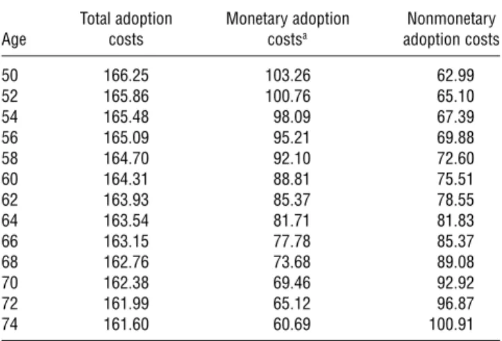
Our estimates of adoption costs may seem surpris-ing because they appear to go against the common belief that the elderly have more difficulties learn-ing or are reluctant to learn new technology, includ-ing the use of ATMs. A more careful examination of our results shows that our findings are consis-tent with previous research. Note that we estimate the total adoption costs, including both monetary and nonmonetary. The monetary costs are the total dis-counted annual fees, whichdecreasewith age because the remaining life span becomes shorter. The non-monetary adoption costs include learning costs, has-sle costs, psychological costs, etc. Given that our esti-mated total adoption costs are fairly flat across age for people over age 50, this implies that the nonmonetary adoption costs increase with age for people over age 50. In Table 9, we show the breakdown of seg-ment 1 consumers’ total adoption costs into mone-tary and nonmonemone-tary components. To calculate the monetary component, we set the average annual fee at E7.32.29 Our results show that monetary adop-tion costs decrease with age, and nonmonetary costs generally increase with age. For example, a 50-, 64-, and 74-year-old person’s nonmonetary adoption costs (measured in monetary terms) areE62.99,E81.83, and E100.91, respectively, if they belong to segment 1.
6.3.4. How Does the Estimate of Adoption Costs Vary with Discount Factor? As mentioned earlier, how consumers discount the future can be context specific. Hence, even though we fix the discount
29Attanasio et al. (2002) report that the average annual fee isE6.2
(1995 base). Because all of our monetary variables are expressed in 2002 euros, we convert the annual fee to 2002 base when calculating monetary adoption costs.
Table 9 A Breakdown of Segment 1 Consumers’ Total Discounted Adoption Costs
Total adoption Monetary adoption Nonmonetary
Age costs costsa adoption costs
50 166.25 103026 62099
52 165.86 100076 65010
54 165.48 98009 67039
56 165.09 95021 69088
58 164.70 92010 72060
60 164.31 88081 75051
62 163.93 85037 78055
64 163.54 81071 81083
66 163.15 77078 85037
68 162.76 73068 89008
70 162.38 69046 92092
72 161.99 65012 96087
74 161.60 60069 100091
Note. Measured in 2002 euros.
aMonetary adoption costs: Discounted annual fees up to the terminal age
based on annual fee=7.32 euros, and=00943.
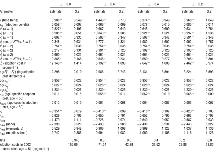
factor using a survey question that specifically solic-its time preferences, consumers may consider future benefits differently in the case of ATM card adop-tion. Therefore, we re-estimate our model by fixing the discount factors at a range of additional val-ues: 0.8, 0.6, 0.4, and 0.2. The results are reported in Table 10. As expected, as we decrease the dis-count factor the age-specific component of adoption costs for the elderly (old5becomes increasingly more positive and significant. The corresponding estimated adoption cost moves in the opposite direction; i.e., it increases with the discount factor. To illustrate this result, we report the adoption cost of segment 1 con-sumers at age=51 in the last row of the table. It shows that the adoption cost increases from E28.85
(=0) to E166.06 (=00943). This suggests that as
long as consumers are forward-looking (i.e., >0), ignoring the heterogeneous life span could lead to biased estimates in adoption costs for different age groups and, possibly, misleading policy implications.
6.4. Counterfactual Experiments
It has been argued that banks’ adoption of finan-cial innovations such as ATMs can improve their productivity in general. ATMs allow banks to pro-cess cash withdrawals and deposits at significantly lower marginal costs than tellers, and potentially bet-ter serve their customers’ basic needs. (For example, a bank can install ATMs in different locations more cheaply than opening brick-and-mortar branches, and ATMs can operate 24 hours a day and seven days per week.) If most customers use ATMs to conduct withdrawal and deposit transactions, bank tellers can shift their focus to help customers with more compli-cated transactions, which could potentially be more profitable for banks. With more customers adopting