``Mixed Duopoly: Differential Game Approach'', mimeo (with Koichi Futagami and Toshihiro Matsumura)

KIER DISCUSSION PAPER SERIES

KYOTO INSTITUTE

OF

ECONOMIC RESEARCH

KYOTO UNIVERSITY

KYOTO, JAPAN

Discussion Paper No.969

“Mixed Duopoly: Differential Game Approach”

Koichi Futagami Toshihiro Matsumura Kizuku Takao

April 2017

Mixed Duopoly: Differential Game Approach ^∗

Koichi Futagami

Toshihiro Matsumura

Kizuku Takao

April 4, 2017

Abstract

Previous studies in differential games reveal that intertemporal strategic behav- iors have an important role for various economic problems. However, most of their analyses are limited to cases where objective functions are identical among agents. In this paper, we characterize the open-loop Nash equilibrium and the Markov perfect Nash equilibrium of a mixed duopoly game where a fully or partially state-owned firm and a fully private firm compete in the quantities of homogeneous goods with sticky prices. We show that in the Markov perfect Nash equilibrium, an increase in the governments’ share-holdings of the state-owned firm has a non-monotonic effect on the price, and in a wide range of parameter spaces, it increases the price. These results are derived from the interaction of an asymmetric structure of agents’ objec- tives and inter-temporal strategic behaviors, which are in sharp contrast with those in the open-loop Nash equilibrium. We provide new implications for privatization policies in the presence of dynamic interactions, against the static analyses.

Keywords: Mixed Duopoly, Open-loop Nash equilibrium, Markov Perfect Nash equi- librium

∗We would like to thank Hiroaki Ino, Takayuki Oishi, and the seminar participants at the EARIE 2016, Macroeconomic policy workshop on Hosei University, and Kwansei Gakuin University. Futagami’s research is partially supported by the Japan Society for the Promotion of Science (JSPS) through a Grant-in-Aid for Scientific Research (B) (No. 15H03355). Takao’s research is partially supported by the Japan Society for the Promotion of Science (JSPS) through Grant-in-Aid for Research Activity start-up (No. 15H065240) and the Joint Research Program of KIER, Kyoto University. All remaining errors are ours.

†Graduate School of Economics, Osaka University, 1-7 Machikaneyama, Toyonaka, Osaka 560-0043, JAPAN; e-mail: futagami@econ.osaka-u.ac.jp

‡Institute of Social Science, The University of Tokyo, 7-3-1, Bunkyo-ku, Hongo, Tokyo, 113-0033, Japan; e-mail:matsumur@iss.u-tokyo.ac.jp

§Corresponding author. Department of Economics, Aomori Public University, 153-4 Aza Yamazaki, Oaza Goushizawa Aomori City, Aomori 030-0196 Japan; e-mail: kizukutakao@gmail.com

JEL classification: C73, D43, L32

1 Introduction

Differential game approaches are widely applied to a number of studies in many fields of economics. These consist of two Nash equilibrium concepts: the open-loop Nash equilib- rium (hereafter referred to as OLNE) and the Markov perfect Nash equilibrium (hereafter referred to as MPNE).¹ Importantly, the MPNE is subgame perfect and takes into accounts of inter-temporal strategic behaviors among agents.² The seminal paper by Fershtman and Kamien (1987) characterizes the OLNE and the MPNE of the Cournot game with a sticky price. They reveal that in the MPNE the presence of inter-temporal strategic substi- tutability makes firms produce more aggressively compared with the static game. Other subsequent studies also shed light on the importance of inter-temporal strategic behaviors for various economic problems. However, most of the previous studies are limited to sym- metric cases where objective functions are identical among agents. If objective functions are asymmetric among agents, the analysis of differential games becomes substantially difficult.

In this paper, we tackle this problem. Specifically, we consider a differential game of a mixed duopoly market where a fully or partially state-owned firm (hereafter referred to as firm 1) and a fully private firm (hereafter referred to as firm 2) compete in the quantity of homogeneous goods.³ Here we explicitly allow the possibility of partial privatization along the lines of Matsumura (1998). That is, we assume that the government can indirectly control the weight of the payoff in firm 1’s objective function through its share-holdings.

1The MPNE is often referred to as a feedback (or closed-loop) Nash equilibrium.

2Cabral (2012) points out the importance of considering issues in an area of industrial organization by using dynamic models. Note that the OLNE is not subgame perfect and does not takes into account inter-temporal strategic behaviors among agents. By definition, in the OLNE, each player chooses an entire time path of his/her actions at the outset of the game given the entire path strategy chosen by the other player. On the other hand, in the MPNE, each firm chooses its strategy at each point in time after observing the value of its payoff-relevant state variables. See Dockner, Jorgensen, Long, and Sorger (2000) for more detailed explanations of differential games.

3Mixed markets are found especially in regulated industries such as transport services, utilities, medical care, finance and insurance, broadcasting, and heavy manufacturing industry. Since the 1980’s, we have also observed a worldwide trend toward privatization of state-owned firms. Whether or not privatization policy is beneficial to social welfare has long been debated. Starting from the seminal papers developed by De Fraja and Delbono (1989) and Matsumura (1998), many researchers have examined this issue in the context of static oligopoly theory by incorporating various related ingredients. Introduction in Matsumura and Shimizu (2010) provide excellent surveys for literature of mixed oligopoly.

Firm 1 maximizes discounted streams of the weighted average of social welfare and profits, whereas firm 2 does discounted streams of profits. Thus, unless firm 1 is perfectly priva- tized, this game has an asymmetric structure of agents’ objectives. Formally, by assuming price stickiness of the homogeneous goods in a similar way to the literature of differential games [e.g. Fershtman and Kamien (1987), Piga (2000), and Cellini and Lambertini (2004, 2007)], we characterize the OLNE and the MPNE of the mixed market on an infinite time horizon. Then we examine how privatization of firm 1 affects firms’ production behaviors, equilibrium price, and social welfare.

We have the following results. First, we analytically show that in the OLNE, an increase in the governments’ share-holdings of firm 1 monotonically reduces the equilibrium price. This is because firm 1 aggressively expands output levels in order to enhance consumer surplus, which is enough to compensate output contractions by the other fully private firm. Our numerical analyses show that neither fully privatization nor fully nationalization is optimal for social welfare, and that the optimal degree of privatization is low. These results are consistent with in the static Nash equilibrium [see De Fraja and Delbono (1989) and Matsumura (1998)]. Second, more importantly, we numerically show that in the MPNE, an increase in the governments’ share-holdings of firm 1 has a non-monotonic effect on equilibrium price. Furthermore, in a wide range of parameter spaces, it leads to higher equilibrium price. These results are derived from the interaction of an asymmetric structure of agents’ objectives and inter-temporal strategic behaviors. When the governments’ share- holdings of firm 1 increase, firm 1 intends to expand output levels in order to enhance consumer surplus. However, firm 1 now expects that if firm 1 expands outputs today, it leads to lower prices tomorrow, which gives incentives for firm 2 to contract output levels tomorrow. Taking such inter-temporal effects into account, firm 1 refrains from aggressively expanding outputs. Such modest output expansions by firm 1 are not enough to compensate output contractions by firm 2. As a result, an increase in government participation in firm 1 raises the price, which is in sharp contrast to the results in the literature on mixed oligopolies that is based on static analysis.

This surprising result brings about an important policy implication. Such a price rise can reduce welfare, and thus, the government has a stronger incentive for reducing gov-

ernment participation in the presence of dynamic interactions. As a result, the optimal degree of privatization is higher in the MPNE than in the OLNE and in the static equilib- rium. This implies that if state-owned firms face dynamic competition with private firms and firms take into account inter-temporal strategic effects, the government privatizes the state-owned firm more. It suggests that the traditional static analysis in the literature on mixed oligopolies may underevaluate the value of privatization.⁴

The rest of the paper is organized as follows. Section 2 describes the model. Section 3 characterizes the Open-loop Nash equilibrium and the Markov perfect Nash equilibrium. Section 4 analyzes the steady-state equilibrium as well as the corresponding transitional dynamics.

2 Model setup

We consider the following duopoly model. Homogeneous goods are produced by two firms: a fully or partially state-owned firm and a fully private firm. They compete in the quantities

´a la Cournot fashion with each other. The differences of the two firm forms are hereafter described in detail. For brevity of exposition, in what follows, we call the fully or partially state-owned firm as firm 1 and the fully private firm as firm 2. Time is continuous and is denoted by t ∈ [0, ∞). The cost function of the both firms is symmetric, which is given by

C (xi(t)) = cxi(t) +¹ 2^xi(t)

2_{, i = 1, 2, (1)}

where c ≥ 0 and xi(t) is the output levels of firm i at time t.⁵ Along the lines of the literature in differential game theory [e.g. Simman and Takayama (1978), Fershtman and Kamien (1987), Piga (2000), and Cellini and Lambertini (2004, 2007)], we consider the price stickiness in the homogeneous goods market. The price of the homogeneous goods,

4There are other approaches of long-run competition in mixed oligopolies. One is the analysis free-entry markets (Anderson, de Palma, and Thisse,1997; Matsumura and Kanda, 2005). Another is the analysis of repeated game (Colombo, 2016). These approach are completely different from ours.

5The assumption of quadratic cost functions is popular in the literature on mixed oligopolies (De Fraja and Delbono, 1989). If both firms have the same cost function and the marginal costs are constant, the monopoly by the state-owned firm obviously yields the first best outcome. Thus, it is nonsense to discuss mixed oligopolies in such a situation. We do not allow cost asymmetry between two firms for tractability.

p(t), is governed by the following differential equation: dp(t)

dt ^≡

p•_t= s [a − X(t) − p(t)] , 0 < c < a, (2)

where X(t) ≡ x1(t) + x2(t) represents total outputs and 0 < s ≤ ∞ represents the degree of the speed of the price adjustments.

Under this environment, the consumer surplus at each point in time, CS(t), is given by

CS(t) ≡

∫ z=X(t) z=0

(a − X(t)) dz − p(t)X(t) = aX(t) − ¹ 2^X(t)

2− p(t)X(t), (3)

and the producer surplus which consists of profits of the both firms at each point in time, P S(t), is given by

P S(t) ≡ p(t)x1(t) − C (x1(t)) + p(t)x2(t) − C (x2(t)) . (4)

The social welfare (total surplus) at each point in time, SW (t), is defined to be the sum of the consumer surplus and the producer surplus:

SW (t) = CS(t) + P S(t). (5)

Following Matsumura (1998), we assume that the government may own some or all parts of the share of firm 1. The government is benevolent to maximize the social welfare. Firm 1’s objective is to maximize the discounted streams of the weighted average of the social welfare and its own profit. The objective functional of firm 1 is given by

V1 =

∫ t=∞ t=0

[βSW (t) + α {p(t)x1(t) − C (x1(t))}] e^−rtdt, α + β = 1, (6)

where r > 0 represents the exogenous constant inter-temporal discount rate and β repre- sents the weight of the payoff of the government for firm 1’s objective. The government can control the value of β(= 1 − α) through its share-holding. An increase in the government’s share-holdings of firm 1 means a higher value of β. By contrast, firm 2’s objective is to

maximize the discounted stream of its own profit. We assume that β = 1 (β = 0) if the government owns 100% (0%) share in firm 1. The objective functional of firm 2 is given by:

V2 =

∫ t=∞ t=0

[p(t)x2(t) − C (x2(t))] e^−rtds. (7)

3 Nash equilibrium

We characterize the OLNE and the MPNE of the mixed duopoly game. Before observing this, we briefly note how outcomes are determined in the static (one-shot) mixed duopoly game, along the lines of the environment as described in the preceding section [see Mat- sumura (1998) for more general characterization].

3.1 Static Nash equilibrium

Here, the time subscript can be dropped. The corresponding inverse-demand function is given by p = a − (x1+ x2). Firm 1’s objective is to maximize βSW + α [px1− C(x1)] with respect to x1, and firm 2’s objective is to maximize px2− C(x2) with respect to x2. The first-order condition of firm 1 is given by

α ^∂p

∂x₁^{x1+ p − C}

′(x1) = 0, (8)

and the first-order condition of firm 2 is given by

∂p

∂x2

x2+ p − C^′(x2) = 0. (9)

Solving (8) and (9) yield the following reaction function of firm 1 and firm 2: x1 = (a − c − x2)/(3 − β) and x2 = (a − c − x1)/3. Therefore, we obtain the following proposition: Proposition 1. Let p^∗ST, x^∗₁^ST, and x^∗₂^ST denote the price, the output levels of firm 1, and the output levels of firm 2 in the Static Nash equilibrium (hereafter referred to as STNE), respectively. We obtain that:

• p^∗ST is given by

p^∗ST = −β(2a + c) + 4(a + c)

8 − 3β ^{. (10)}

• x^∗₁^ST and x^∗₂^ST are given by

x^∗₁^ST = ^{2(a − c)}

8 − 3β ^{, (11)}

x^∗₂^ST = (2 − β)(a − c)

8 − 3β ^{. (12)}

• For β ∈ [0, 1], x^∗₁^ST is increasing in β, whereas x^∗₂^ST and p^∗ST are decreasing in β.

• For β ∈ [0, 1], let ˆβ be the value of β that maximizes the social welfare in the STNE, SW^∗ST(β). It is found that ˆβ ∈ (0, 1).

Proof. The first to third results are straightforwardly derived by simple calculations using (2), (8), and (9). We briefly give the proof for the last result. SW^∗(β) is given by

SW^∗ST(β) =

∫ x^∗ST1 (β)+x^∗ST2 (β) 0

p(q)dq − C⁽x^∗₁^ST(β)⁾− C⁽x^∗₂^ST(β)⁾.

From (11) and (12), differentiating SW^∗ST(β) with respect to β in the neighborhood of β = 0 yields

∂SW^∗ST(β)

∂β  

β=0

=^[p − C^′(x^∗₁^ST)^]

| {z }

(+)

∂x^∗₁^ST(β)

∂β  

β=0

| {z }

(+)

+^[p − C^′(x^∗₂^ST)^]

| {z }

(+)

∂x^∗₂^ST(β)

∂β  

β=0

| {z }

(−)

= ^{(a − c)}

2

8 ^{> 0.}

On the other hand, differentiating SW^∗ST(β) with respect to β in the neighborhood of β = 1 yields

∂SW^∗ST(β)

∂β  

β=1

=^[p − C^′(x^∗₁^ST)^]

| {z }

=0

∂x^∗₁^ST(β)

∂β  

β=1

+^[p − C^′(x^∗₂^ST)^]

| {z }

(+)

∂x^∗₂^ST(β)

∂β  

β=1

| {z }

(−)

< 0,

where the first term is equal to 0 and the second term is negative.

As the third result in Proposition 1 shows, firm 1’s output levels are monotonically increasing in β, whereas firm 2’s output levels are monotonically decreasing in β. As β increases, however, the output expansion by firm 1 always compensates the output contraction by firm 2. Therefore, the price is monotonically decreasing in β. The last result in Proposition 1 indicates that neither full privatization nor full nationalization is optimal. The reason is explained as follows. If β = 0, price declines by a marginal increase in β necessarily improves social welfare because the price level is too high in the presence of imperfect market competition. On the other hand, if β = 1, a slight reduction in output levels of firm 1 does not reduce social welfare as the price is equal to the marginal cost for firm 1. However, because the price is higher than the marginal cost for firm 2, a marginal increase in the outputs of firm 2 caused by a decrease in β improves social welfare. We provide another intuitive explanation behind this result by using the welfare-improving production substitution discussed by Lahiri and Ono (1988). An increase in β reduces the price and mitigate distortion due to imperfect market competition. On the other hand, an increase in β increases the output of firm 1 and reduces that of firm 2 (production substitution from firm 2 to firm 1). When β is positive, firm 1 produces more than firm 2, and thus, the marginal cost is higher in firm 1 than in firm 2. Therefore, this production substitution harms social welfare. The latter (former) dominates the former (latter) when β = 1 (β = 0), and thus, neither β = 0 nor β = 1 is optimal for social welfare. As shown below in section 4, however, an increase in β can raise the price at the MPE, especially when β is large. Thus, the optimal degree of privatization is lower at the MPNE.

3.2 Open-Loop Nash equilibrium

In this subsection, we characterize the OLNE for the above-mentioned game. The open- loop information set for each firm is defined by only its own actions and time. No firm can observe anything but those items at each point in time. As we will see below, the open-loop information set is more narrow than the Markov perfect information set. The open-loop strategy of each firm is characterized by the entire time path for the control variable (its own outputs), which is fixed at the outset of the game given the rival’s strategy and the

initial level of the state variable (price). Each firm commits to the path and does not revise it at any subsequent point in time. Hence, the actions to be done at each point in time depends only on the time. Formally, following Fershtman and Kamien (1987), we define the open-loop strategy space and the OLNE for the game as follows:

Definition 1. The open-loop strategy space for firm i (i = 1, 2) is

S_i^OP = {xi(t) | xi(t) is piecewise continuous and xi(t) ≥ 0 for every t}.

Definition 2. The open-loop Nash equilibrium (OLNE) is a pair of the open-loop strategies, (x^∗₁^OP(t), x^∗₂^OP(t)) ∈ S₁^OP × S₂^OP such that

Vi

(x^∗_i^OP(t), x^∗_j^OP(t)⁾ ≥ Vi

(xi(t), x^∗_j^OP(t)⁾ for every xi(t) ∈ S_i^OP (i, j = 1, 2 ; i ̸= j) .

We solve the OLNE by using Pontryagin’s maximum principle and derive the following proposition:

Proposition 2. Let p^∗OP(∞), x^∗₁^OP(∞), and x^∗₂^OP(∞) respectively denote the steady-state price, the steady-state output levels of firm 1, and the steady-state output levels of firm 2 in the OLNE. We obtain that

• There is a unique and globally stable steady-state in the OLNE.

• p^∗OP(∞) is given by

p^∗OP(∞) = [as + (a + 2c)(r + s)] (r + 2s) − βs [as + (a + c)(r + s)] (3r + 4s)(r + 2s) − βs(2r + 3s) ^.

• x^∗₁^OP(∞) is given by

x^∗₁^OP(∞) = (a − c)(r + s)(r + 2s) (3r + 4s)(r + 2s) − βs(2r + 3s)^.

• x^∗₂^OP(∞) is given by

x^∗₂^OP(∞) = (a − c)(r + s) [(r + 2s) − βs] (3r + 4s)(r + 2s) − βs(2r + 3s)^.

• For β ∈ [0, 1], x^∗₁^OP(∞) is increasing in β, whereas p^∗OP(∞) and x^∗₂^OP(∞) are decreasing in β.

Proof. See Technical Appendix A-1.

The last result in Proposition 2 indicates that an increase in the government’s share- holdings of firm 1 unambiguously leads to the lower steady-state price at the OLNE. This is because output expansions by firm 1 necessarily compensate output reductions by firm 2. These are qualitatively consistent with the result of the STNE. Although the welfare implication cannot be derived analytically, as shown by numerical analyzes in the subsequent section, we also confirm that welfare implications at the steady state in the OLNE are qualitatively consistent with the STNE.

Besides, the following two extreme parameter cases are considered along the lines of the literature of the differential game theory [e.g. Fershtman and Kamien (1987), Piga (2000) and Cellini and Lambertini (2004, 2007)]. One is the case in which s → ∞ or r → 0 (referred to as the “limit game”). In this case, the steady state of the game can be viewed as a continuous-time version of the repeated game. The second is the case in which s → 0 or r → ∞. In this case, each firm chooses its own strategy under the situation where the price is perfectly rigid or only its current profit flow is important. We obtain the following proposition:

Proposition 3. As s → ∞ or r → 0, p^∗OP(∞) coincides with the price in the STNE, p^∗ST. On the other hand, as s → 0 or r → ∞, p^∗OP(∞) coincides with the static competitive price which is given by (a + 2c)/3.

Proof. From Proposition 2, taking the limit of s → ∞ or r → 0 (s → 0 or r → ∞) for p^∗OP(∞), we straightforwardly obtain the results above.

3.3 Markov Perfect Nash equilibrium

In the following, we characterize the MPNE for the above-mentioned game. The Markov perfect information set is less restricted compared to the OLNE in that each firm can observe the realization value of the payoff-relevant state variable (price) at each point in

time. In contrast to the OLNE, each firm does not commit to a particular time path of its control variable at the outset of the game, but rather, each firm can respond to the observed price level at each point in time. As a result, the Markov perfect strategies of the firms are the decision rules which prescribe the firm’s outputs at each point in time as a function of the observed price. Formally, following Fershtman and Kamien (1987), the Markov perfect strategy and the MPNE are defined as follows:

Definition 3. The Markov perfect strategy space for firm i (i = 1, 2) is

S_i^{M P} = {xi(t, p(t)) | xi(t, p(t)) is continuous in (t, p(t)) ; xi(t, p(t)) ≥ 0 and

|xi(t, p(t)) − xi(t, p^′(t)) | ≤ m(t)|p(t) − p^′(t)| for some integrable m(t) ≥ 0}.

Definition 4. The Markov perfect Nash equilibrium (MPNE) for the game is a pair of the Markov perfect strategies, (x^∗₁^{M P}(t, p(t)) , x^∗₂^{M P}(t, p(t))) ∈ S₁^{M P}× S₂^{M P} such that for every possible initial condition (t0, p(t0)),

Vi

(x^∗_i^{M P}(t, p(t)) , x^∗_j^{M P}(t, p(t))⁾≥ Vi

(xi(t, p(t)) , x^∗_j^{M P}(t, p(t))⁾,

for every xi(t, p(t)) ∈ S_i^{M P} (i, j = 1, 2 ; i ̸= j) .

The MPNE can be solved by dynamic programming. To make exposition simple, in what follows, we omit the time subscript. The Markov perfect Nash equilibrium strategies, {x^∗₁^{M P}(p), x^∗₂^{M P}(p)}, must satisfy the following Hamilton-Jacobi-Bellman equations:

rV1(p) = max

x1

[ β

(

aX − ¹ 2^X

2

)

+ αpx1− (

cx1+ ¹ 2^x

2 1

)

− β (

cx2+ ¹ 2^x

2 2

)

+ ^∂V1(p)

∂p s (a − X − p) ]

, (13)

rV2(p) = max

x2

[ px2−

(

cx2+ ¹ 2^x

2 2

)

+^∂V2(p)

∂p s (a − X − p) ]

. (14)

The first-order conditions for (13) and (14) are respectively given by

β {a − X} + αp − (c + x1) − s^∂V1(p)

∂p ^{= 0, (15)}

p − c − x2− s^∂V2(p)

∂p ^{= 0. (16)}

We guess the value function of firm i as the following quadratic form:

Vi = ¹ 2^Kip

2 _{+ E}

ip + Fi (i = 1, 2), (17)

where {Ki, Ei, Fi} (i = 1, 2) are undetermined coefficients. From (15), (16), and (17), we obtain the following linear Markov-perfect strategies⁶:

Proposition 4. The Markov perfect Nash equilibrium strategies, ⁽x^∗₁^{M P}(p), x^∗₂^{M P}(p)⁾, are respectively given by

x^∗₁^{M P}(p) = ¹

1 + β [(1 − 2β − sK1+ βsK2) p + βa − (1 − β)c − sE1+ βsE2] , (18)

x^∗₂^{M P}(p) = (1 − sK2)p − (c + sE2), (19)

where {K1, K2} must satisfy the following simultaneous equations: 1

2(2β + α)^s

2_K2 1 ⁺

1 2β + α^s

2_K

1K2− ^β 2

( 1

2β + α ^{+ 1} )

s²K₂²

−^{[ 3α}

3+ 13αβ + 8β² (2β + α)^{2 s +}

1 2^r

]

K₁+ 3 ^β

2β + α^sK2−

6β³+ 11αβ²+ 2α²β − α³

2(2β + α)^{2 = 0, (20)} 1

2 ⁻ 1 2^rK2+

α 2(2β + α)^s

2_K2 2 ⁺

1 2β + α^s

2_K

1K2− ³

2β + α^{sK2 = 0. (21)}

For {K1, K2} determined by (20)-(21), {E1, E2} must satisfy the following simultaneous equations:

rE₁ = βa(β + 2α) − s(K1+ K2)

2β + α + β [(1 − sK₂)sE₂]

− ^β

(2β + α)² [(β + 2α) − s(K1+ K2)] [(βa − 2c) − s(E1+ E2)]

+ ^α

2β + α[βa − αc − s(E1− βE2)] + ^c

2β + α [(β − α) + s(K1− βK2)]

6Tsutusi and Mino (1990) consider nonlinear strategies in the Fershtman Kamien (1987)’s model. Here we focus only on linear strategies to clarify characters of our dynamic game.

+ ¹

(2β + α)² [(β − α) + s(K1− βK2)] [(βa − αc) − s(E1− βE2)]

+ ¹

2β + α

[(a + 2c)sK1− 3sE1+ 2s²K1E1+ s²(K1E2+ K2E1)^], (22) (

r + ³ 2β + α^s

)

E2 = −c + ¹ 2β + α

[(a + 2c)sK2+ s²(K1E2+ K2E1) − βs²K2E2

]. (23)

Proof. See Technical Appendix A-2.

Note that when β = 0, the RHS of (18) coincides with the RHS of (19). In this case, K₁ = K₂ and E₁ = E₂ are satisfied.⁷ Applying (18) and (19) into X = x₁+ x₂ and (2), the total outputs and the law of motion of price in the MPNE are respectively given by:

X = ¹

1 + β [(2 − β − sK1+ sK2) p + βa − 2c − sE1 + sE2] , (24) p =• ^s

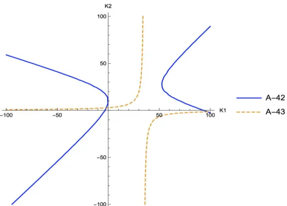
1 + β [− {3 − s(K1+ K2)} p + a + 2c + s(E1 + E2)] . (25) (25) indicates that 3 > s(K1+ K2) must be satisfied so that the pair (x^∗₁^{M P}(p), x^∗₂^{M P}(p)) constitutes the globally and asymptotically stable MPNE. Since it is too complicated to analytically find the equilibrium value of {K1, K2, E1, E2} for the case of β ∈ (0, 1] from (20)-(21) and (22)-(23), we relay on numerical analysis so as to derive our main implications as demonstrated in the subsequent section. Before going to the quantitative analysis, however, we give some analytical results here. First, we obtain the following lemma: Lemma 1. The graph of (20) is a hyperbola.

Proof. See Technical Appendix A-3.

And we can show the following results for the case of β = 1:

Proposition 5. If β = 1, the system of simultaneous equations, (20)-(21), has a unique solution. Moreover, it is found that K1 < 0 and K2 > 0.

Proof. See Technical Appendix A-4.

Second, considering p = 0, we derive the following lemma and proposition:^•

7See Fershtman and Kamien (1987).

Lemma 2. Let p^{∗M P}(∞), x^∗₁^{M P}(∞), and x^∗₂^{M P}(∞) respectively denote the steady-state price, the steady-state output levels of firm 1, and the steady-state output level of firm 2 in the MPNE. We find:

• p^{∗M P}(∞) is given by

p^{∗M P}(∞) = a + 2c + s(E1+ E2)

3 − s(K1+ K2) ^{. (26)}

• x^∗₁^{M P}(∞) is given by

x^∗₁^{M P}(∞) = ¹ 1 + β

[ {1 − 2β − s(K1+ βK2)} {a + 2c + s(E1+ E2)} 3 − s(K1+ K2)

+ βa − (1 − β)c − s(E1− βE2) ]

, (27)

• x^∗₂^{M P}(∞) is given by

x^∗₂^{M P}(∞) = ^{(1 − sK2}) {a + 2c + s(E1+ E2)}

3 − s(K1+ K2) ^{− (c + sE2). (28)}

Proof. Derivations for these results are straightforwardly obtained using (18), (19), (24), and (25).

Proposition 6. As s → 0 or r → ∞, x^∗₁^{M P}(∞) and x^∗₂^{M P}(∞) are equal to (a − c)/3 for any β ∈ [0, 1]; p^{∗M P}(∞) is equal to (a + 2c)/3. That is, the steady-state outcomes in the MPNE coincide with the static competitive equilibrium.

Proof. They are straightforwardly obtained by applying s → 0 or r → ∞ to Lemma 2.

4 Numerical Analysis

4.1 Methodology

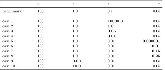
Employing numerical simulations, we examine how an increase in β affects the steady state of the MPNE and the OLNE, as well as considering the transitional dynamics from an arbitrary initial state to the steady state. As a benchmark, we focus on the parameter

set listed in Table 1. We confirm that our main implications derived from the benchmark analysis are fairly robust to a wide range of parameter sets except for the case in which s is extremely low or s is extremely high. Recall that as s → 0 or r → ∞, both the steady states of the MPNE and the OLNE degenerate to the static competitive equilibrium. When s → ∞ or r → 0 (limit price case), the steady state of the OLNE degenerates to the STNE. On the other hand, qualitative implications of the MPNE in the limit price case remain the same as those under the benchmark parameter case. To save space in the text, we relegate the detailed analysis for robustness checks to the Technical Appendix.

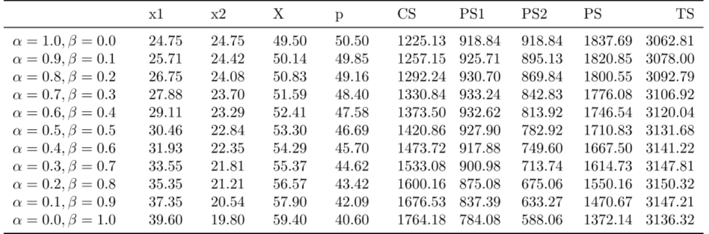
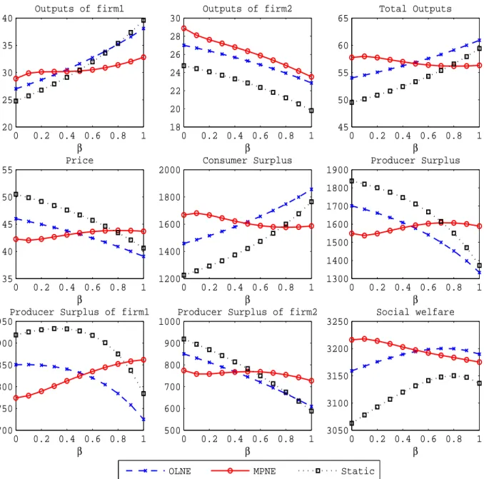
Table 2 summarizes the MPNE strategies computed in increments of 0.1 for β ∈ [0, 1] under the benchmark parameter set. Each panel of Figure 1 respectively displays variations in the steady-state output levels of firm 1 (x1), output levels of firm 2 (x2), total outputs (X), price (p), consumer surplus (CS), producer surplus (PS), profit of firm 1 (PS1), profit of firm 2 (PS2), and social welfare (SW) with respect to β in the MPNE and OLNE under the benchmark parameter set. These are computed in increments of 0.1 for β ∈ [0, 1]. For reference, the corresponding outcomes in the STNE are also displayed on each panel. Table 3-5 numerically list these values.

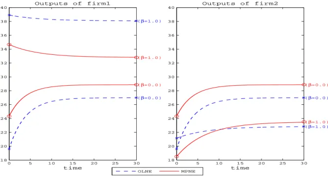
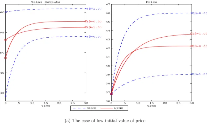
The transitional dynamics are computed by employing the relaxation algorithm method developed by Trimborn, Koch and Steger (2008).⁸ Since a one state variable exists (price), we need to arbitrary set the initial price for computations of the transitional dynamics. As the initial price level, we consider 80% and 120% level of the steady-state price in the OLNE for β = 0.0. Figure 2 respectively displays the transitional dynamics of output levels of firm 1 and firm 2 in the MPNE and the OLNE for β = 0.0, 1.0. In the same manner, Figure 3 respectively displays the transitional dynamics of total outputs and price.

4.2 Model properties

Figure 1 shows that variations in each variable with respect to β in the OLNE are analogous to those in the STNE. In contrast, the MPNE qualitatively and quantitatively exhibits

8Trimborn, Koch, and Steger (2008) detail the relaxation algorithm. They also provide MAT- LAB programs for the relaxation algorithm, which are downloadable for free at http://www.wiwi.uni- siegen.de/vwli/forschung/relaxation/matlab applications.html?lang=de.

different implications of a change in β, compared to in the OLNE and the STNE. Since the production behaviors of firm 1 and firm 2 as a function of β are keys in our paper, in what follows, we first examine them in detail.

4.2.1 Production behavior of firm 1 and firm 2

Figure 1 and Table 3-5 show that for every equilibrium concept, the (steady-state) output levels of firm 1 are increasing in β, whereas the (steady-state) output levels of firm 2 are decreasing in β. But the magnitude of output expansions of firm 1 associated with a higher β in the MPNE is considerably smaller than in the OLNE and the STNE. Note that if β = 0.0, the steady-state output levels of firm 1 in the MPNE are higher than in the OLNE and the STNE. As β exceeds a certain threshold level, however, the steady-state output levels of firm 1 in the MPNE become lower than in the OLNE and the STNE. In contrast, the steady-state output levels of firm 2 in the MPNE is higher than in the OLNE and the STNE for any β ∈ [0, 1]. Furthermore, Figure 2 illustrates that if β = 0.0, firm 1’s output levels and firm 2’s output levels in the MPNE are always higher than in the OLNE during the transitional phase. On the other hand, if β = 1.0, firm 1’s output levels in the MPNE are always lower than in the OLNE. Firm 2’s output levels in the MPNE are lower than in the OLNE during the early stage of the transition, whereas the steady-state firm 2’s output levels in the MPNE are higher than in the OLNE.

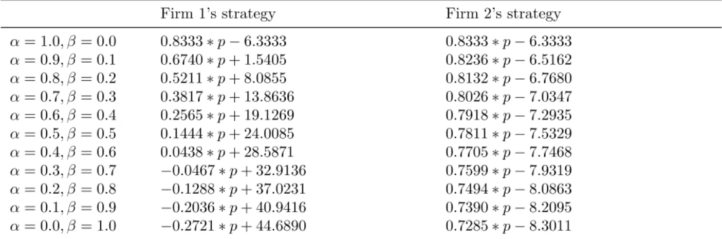
Table 2 shows that as β increases starting from β = 0.0, the Markov perfect Nash equilibrium strategies of firm 1 and firm 2 changes asymmetrically. If β = 0.0, the Markov perfect strategy of both firms is given by 0.8333∗p−6.3333 under the benchmark parameter set. As β increases, the coefficient-value of p in the Markov perfect Nash equilibrium strategy of firm 1 decreases and becomes even negative. By contrast, the intercept-value in the Markov perfect Nash equilibrium strategy of firm 1 is increasing in β. These indicate that firm 1’s behavior drastically changes depending on β. On the other hand, as β increases, the coefficient-value of p in the Markov perfect strategy of firm 2 also decreases but remains to be positive for any β ∈ [0, 1]. And the intercept-value in the Markov perfect strategies of firm 2 is decreasing in β. Therefore, as β increases, firm 2 strategically contracts its output levels given a price level.

The reason behind such counter-intuitive results in the MPNE is derived from the interaction of inter-temporal strategic behavior and an asymmetric structure of firms’ ob- jectives. For better understanding of the intuition, specifically consider first the case of symmetric situation (β = 0.0) in order to clarify only the inter-temporal strategic behavior which pertains to the MPNE.⁹ If β = 0, for every equilibrium concept, both firms sym- metrically seek only profits. In the MPNE, both firms strategically intend to make the other firm contract outputs for each other. That is, inter-temporal strategic substitutabil- ity exists. More specifically, at any point in time, if firm i increases outputs today, it leads to lower prices tomorrow. This causes firm j to contract outputs tomorrow, resulting in larger residual demand for firm i. Firm i strategically takes such inter-temporal effects into account and the same logic also prevails in firm j. By definition, such inter-temporal strategic decisions do not occur in the OLNE and the STNE. Therefore, in the MPNE, both firms produce more aggressively compared with the OLNE and the STNE.

Next, consider the case in which β ∈ (0, 1]. As β increases, regardless of equilibrium concepts, firm 1 intends to expand outputs in order to enhance consumer surplus which is distorted by the presence of the imperfect market competition. In contrast, firm 2 remains to seek only its own profits. In the MPNE, however, the presence of inter-temporal strategic decision dampens its incentives for firm 1 to expand outputs due to the asymmetric structure of the firms’ objectives. More specifically, at any point in time, if firm 1 expands outputs today, this leads to lower prices tomorrow, which causes firm 2 to contract outputs tomorrow. This secondary effect will weaken price reduction by firm 1’s outputs expansion. Firm 1 takes such an inter-temporal effect into account, leading to its strategic modest production. Therefore, the magnitude of output expansion of firm 1 associated with higher β in the MPNE is considerably smaller than in the OLNE and the STNE.

In an analogous way, in the MPNE, firm 2 expects that if the price decreases tomorrow, firm 1 will expand outputs tomorrow. This is because the coefficient-value of price in the linear Markov strategy of firm 1 becomes negative as β increases. Taking such inter- temporal effects into account, firm 2 also strategically contracts outputs compared with the OLNE and the STNE. As shown in Figure 2, however, this can be found only in the

9See Fershtman and Kamien (1987) for more description.

early stage of transition. This is because the price around the steady state in the MPNE is higher than in the OLNE and the STNE.

4.2.2 Total outputs and price

Figure 1 and Table 3-5 show that the steady-state price (total output levels) in the OLNE is monotonically decreasing (increasing) in β, which is consistent with outcomes in the STNE. By contrast, in the MPNE, variations in the steady-state price (total outputs) with respect to β is non-monotonic in relationship with β. And surprisingly for a wide range of β, the steady-state price in the MPNE is increasing in β although its variations are quantitatively small. Furthermore, figure 3 shows that if β = 0.0, price (output levels) in the MPNE is always lower (higher) than in the OLNE during all transitional phase, whereas if β = 1.0, the rank order of the configuration inversely changes.

The counter-intuitive result in the MPNE is mainly derived from firm 1’s strategic modest production in reaction to a higher β. In the MPNE, even if β increases, firm 1 refrains from aggressively expanding outputs because of the presence of inter-temporal strategic decision as mentioned above. For a wide range of β, the output expansion by firm 1 associated with higher β cannot compensate the associated output reduction by firm 2. Furthermore, these results directly lead to difference of variations in the steady-state consumer surplus and producer surplus with respect to β. Figure 1 shows that in the OLNE and the STNE, the steady-state consumer surplus (producer surplus) is monotonically increasing (decreasing) in β, whereas the steady-state consumer surplus (producer surplus) in the MPNE is in a non-monotonic relationships with β. And the steady-state consumer surplus (producer surplus) in the MPNE is decreasing (increasing) in β for a wide range of β.

4.2.3 Social welfare

Figure 1 and Table 3-5 show that for every equilibrium concept, the (steady-state) total surplus exhibits an inverted U-shaped relationship with respect to β. This implies that even in the presence of inter-temporal strategic decisions among firms, neither a full privatization policy nor a full nationalization policy is optimal, which is consistent with the preceding

study developed by Matsumura (1998). However, the value of β which maximizes the steady-state total surplus in the MPNE is shown to be quantitatively quite different from the OLNE and the STNE. Specifically, the former value is around β = 0.1, whereas the latter value is around β = 0.7 to β = 0.8. This suggests that in the OLNE and the STNE, the low degree of privatization policy is optimal for the social welfare, whereas in the MPNE, the high degree of privatization policy is optimal for social welfare.

Along the lines of discussions in section 3.1, in the OLNE and the MPNE, there are two channels for a change in β to affect the social welfare. The first channel is via the resulting price change. Since the imperfect competition prevails in the goods market, an equilibrium price is distorted above the social marginal cost. Hence, a price decline has a positive effect on the social welfare. The second channel is via the production substitution among firms associated with a change in β. Since the cost function takes a convex form, the efficiency of the overall production is distorted by asymmetric outputs among firms when β ̸= 0.

In the OLNE and STNE, an increase in β causes firm 1 to aggressively expand output, which monotonically leads to the lower price. The resulting price decline has a positive effect on the social welfare via the first channel. At the same time, the resulting production substitutions from firm 2 to firm 1 has a negative effect on the social welfare via the second channel. Except for the case in which β is near to 1, the extent of positive welfare effects via the first channel exceeds the extent of negative welfare effects via the second channel. As a result, the low degree of privatization policy is optimal for the social welfare.

By contrast, in the MPNE, an increase in β only leads to less aggressive output ex- pansion of firm 1. Figure 1 and Table 3 show that when β is sufficiently low, the price is lower than in the symmetric case (β = 0). On the other hand, the production substitutions occur for any β ∈ [0, 1], as is the case with the OLNE and STNE. As a result, when β is sufficiently low, an increase in β can have a positive welfare effect via the first channel. Therefore, the high degree of privatization policy is optimal for the social welfare. Besides, note that if β = 1.0, the steady-state social welfare in the MPNE is lower than in the OLNE as shown in Figure 1 and Table 3-4. This sharply contrasts with results in the symmetric case which have been examined by Fershtman and Kamien (1987).

5 Conclusion

In this paper, we analyze differential games with asymmetric firms that have different objectives. One is profit maximizer, and the other is concerns with both profits and social welfare. We consider three scenarios: static Nash equilibrium, the open-loop Nash equilibrium, and the Markov perfect Nash equilibrium. We investigate how the weight of social concern in a firm affects the price and social welfare. We find that at the static and open-loop Nash equilibria, an increase in the social concern in a firm’s objective always reduces the price. However, at the Markov perfect Nash equilibrium, it can raise the price. As a result, the optimal degree of social concerns at the Markov perfect Nash equilibrium is substantially lower than those at the static and open-loop Nash equilibria.

In the context of mixed oligopolies in which state-owned public firms compete against private firms, the degree of social concern in a firm’s objective is associated with the public ownership ratio in the firm. Following this interpretation, our result suggests that the optimal degree of privatization is significantly higher at Markov perfect equilibrium than that at the static Nash equilibrium. This implies that when firms face dynamic competition, the government should privatize the state-owned firms more.

In this paper, we take the first step to applying the differential game approach to asymmetric oligopolies in which firms have heterogeneous objectives. For example, firms may be concerned with corporate social responsibility (CSR). In fact, most major firms adopt CSR policies but the degree of CSR significantly differs among firms (KPMG, 2013). We think that our findings can apply to the analysis of such markets. Formal analysis of this problem remains for future research.

Table 1: Benchmark parameter set

a c s r

100 1.0 0.1 0.05

Table 2: Markov perfect Nash equilibrium strategies (benchmark)

Firm 1’s strategy Firm 2’s strategy

α= 1.0, β = 0.0 0.8333 ∗ p − 6.3333 0.8333 ∗ p − 6.3333 α= 0.9, β = 0.1 0.6740 ∗ p + 1.5405 0.8236 ∗ p − 6.5162 α= 0.8, β = 0.2 0.5211 ∗ p + 8.0855 0.8132 ∗ p − 6.7680 α= 0.7, β = 0.3 0.3817 ∗ p + 13.8636 0.8026 ∗ p − 7.0347 α= 0.6, β = 0.4 0.2565 ∗ p + 19.1269 0.7918 ∗ p − 7.2935 α= 0.5, β = 0.5 0.1444 ∗ p + 24.0085 0.7811 ∗ p − 7.5329 α= 0.4, β = 0.6 0.0438 ∗ p + 28.5871 0.7705 ∗ p − 7.7468 α= 0.3, β = 0.7 −0.0467 ∗ p + 32.9136 0.7599 ∗ p − 7.9319 α= 0.2, β = 0.8 −0.1288 ∗ p + 37.0231 0.7494 ∗ p − 8.0863 α= 0.1, β = 0.9 −0.2036 ∗ p + 40.9416 0.7390 ∗ p − 8.2095 α= 0.0, β = 1.0 −0.2721 ∗ p + 44.6890 0.7285 ∗ p − 8.3011

Table 3: Steady-state outcomes in the MPNE (benchmark)

x1 x2 X p CS PS1 PS2 PS TS

α= 1.0, β = 0.0 28.87 28.87 57.75 42.25 1667.53 774.21 774.21 1548.42 3215.95 α= 0.9, β = 0.1 29.86 28.10 57.97 42.02 1680.31 779.41 758.14 1537.56 3217.87 α= 0.8, β = 0.2 30.11 27.61 57.72 42.27 1666.22 789.48 758.40 1547.88 3214.10 α= 0.7, β = 0.3 30.14 27.19 57.34 42.65 1644.32 801.30 763.03 1564.34 3208.67 α= 0.6, β = 0.4 30.17 26.78 56.95 43.04 1622.21 813.24 767.39 1580.64 3202.85 α= 0.5, β = 0.5 30.27 26.35 56.62 43.37 1603.22 824.59 769.41 1594.01 3197.24 α= 0.4, β = 0.6 30.50 25.87 56.37 43.62 1588.89 835.04 768.17 1603.22 3192.11 α= 0.3, β = 0.7 30.86 25.34 56.21 43.78 1579.87 844.33 763.31 1607.65 3187.53 α= 0.2, β = 0.8 31.37 24.77 56.15 43.84 1576.41 852.18 754.76 1606.95 3183.37 α= 0.1, β = 0.9 32.01 24.16 56.18 43.81 1578.54 858.19 742.69 1600.85 3179.38 α= 0.0, β = 1.0 32.80 23.52 56.32 43.67 1586.15 861.90 727.17 1589.08 3175.23

Table 4: Steady-state outcomes in the OLNE (benchmark)

x1 x2 X p CS PS1 PS2 PS TS

α= 1.0, β = 0.0 27.00 27.00 54.00 46.00 1458.00 850.50 850.50 1701.00 3159.00 α= 0.9, β = 0.1 27.80 26.69 54.50 45.49 1485.43 850.67 831.49 1682.17 3167.60 α= 0.8, β = 0.2 28.66 26.37 55.04 44.95 1514.84 849.24 811.55 1660.80 3175.63 α= 0.7, β = 0.3 29.58 26.03 55.61 44.38 1546.43 845.90 790.60 1636.51 3182.94 α= 0.6, β = 0.4 30.55 25.66 56.22 43.77 1580.47 840.27 768.57 1608.85 3189.32 α= 0.5, β = 0.5 31.59 25.27 56.87 43.12 1617.23 831.90 745.39 1577.30 3194.53 α= 0.4, β = 0.6 32.70 24.85 57.56 42.43 1657.05 820.25 720.96 1541.22 3198.27 α= 0.3, β = 0.7 33.90 24.41 58.31 41.68 1700.32 804.64 695.21 1499.85 3200.18 α= 0.2, β = 0.8 35.18 23.92 59.11 40.88 1747.50 784.26 668.02 1452.29 3199.78 α= 0.1, β = 0.9 36.57 23.40 59.98 40.01 1799.11 748.10 639.30 1397.41 3196.52 α= 0.0, β = 1.0 38.07 22.84 60.92 39.07 1855.81 724.92 608.93 1333.86 3189.67

Table 5: Steady-state outcomes in the static game (benchmark)

x1 x2 X p CS PS1 PS2 PS TS

α= 1.0, β = 0.0 24.75 24.75 49.50 50.50 1225.13 918.84 918.84 1837.69 3062.81 α= 0.9, β = 0.1 25.71 24.42 50.14 49.85 1257.15 925.71 895.13 1820.85 3078.00 α= 0.8, β = 0.2 26.75 24.08 50.83 49.16 1292.24 930.70 869.84 1800.55 3092.79 α= 0.7, β = 0.3 27.88 23.70 51.59 48.40 1330.84 933.24 842.83 1776.08 3106.92 α= 0.6, β = 0.4 29.11 23.29 52.41 47.58 1373.50 932.62 813.92 1746.54 3120.04 α= 0.5, β = 0.5 30.46 22.84 53.30 46.69 1420.86 927.90 782.92 1710.83 3131.68 α= 0.4, β = 0.6 31.93 22.35 54.29 45.70 1473.72 917.88 749.60 1667.50 3141.22 α= 0.3, β = 0.7 33.55 21.81 55.37 44.62 1533.08 900.98 713.74 1614.73 3147.81 α= 0.2, β = 0.8 35.35 21.21 56.57 43.42 1600.16 875.08 675.06 1550.16 3150.32 α= 0.1, β = 0.9 37.35 20.54 57.90 42.09 1676.53 837.39 633.27 1470.67 3147.21 α= 0.0, β = 1.0 39.60 19.80 59.40 40.60 1764.18 784.08 588.06 1372.14 3136.32

0 0.2 0.4 0.6 0.8 1 20

25 30 35 40

Outputs of firm1

β ^{0 0.2 0.4 0.6 0.8 1}

18 20 22 24 26 28 30

Outputs of firm2

β ^{0 0.2 0.4 0.6 0.8 1}

45 50 55 60 65

Total Outputs

β

0 0.2 0.4 0.6 0.8 1 35

40 45 50 55

Price

β ^{0 0.2 0.4 0.6 0.8 1}

1200 1400 1600 1800 2000

Consumer Surplus

β ^{0 0.2 0.4 0.6 0.8 1}

1300 1400 1500 1600 1700 1800 1900

Producer Surplus

β

0 0.2 0.4 0.6 0.8 1 700

750 800 850 900 950

Producer Surplus of firm1

β ^{0 0.2 0.4 0.6 0.8 1}

500 600 700 800 900 1000

Producer Surplus of firm2

β ^{0 0.2 0.4 0.6 0.8 1}

3050 3100 3150 3200 3250

Social welfare

β

OLNE MPNE Static

Figure 1: Comparison of the (steady-state) outcomes for alternative equilibrium concept under benchmark parameter case

0 5 10 15 20 25 30 18

20 22 24 26 28 30 32 34 36 38 40

Outputs of firm1

time

(β=0.0) (β=0.0) (β=1.0)

(β=1.0)

0 5 10 15 20 25 30

18 20 22 24 26 28 30 32 34 36 38 40

Outputs of firm2

time

(β=0.0) (β=0.0)

(β=1.0) (β=1.0)

OLNE MPNE

(a) The case of low initial value of price

0 5 10 15 20 25 30

22 24 26 28 30 32 34 36 38 40 42

Outputs of firm1

time

(β=0.0) (β=0.0) (β=1.0)

(β=1.0)

0 5 10 15 20 25 30

22 24 26 28 30 32 34 36 38 40 42

Outputs of firm2

time

(β=0.0) (β=0.0)

(β=1.0) (β=1.0)

OLNE MPNE

(b) The case of high initial value of price

Figure 2: Comparison of transitional path of outputs of firm1 and firm2 in the MPNE and OLNE. The x-marks on the left (right) vertical axis indicates the initial value (steady-state value) in the OLNE. The circle-marks on the left (right) vertical axis indicates the initial value (steady-state value) in the MPNE. In the panel (a), we set initial value of price as 80% level of the steady-state price for β = 0.0 in the OLNE. In the panel (b), we set initial value of price as 120% level of the steady-state price for β = 0.0 in the OLNE.

0 5 10 15 20 25 30 40

45 50 55 60

Total Outputs

time

(β=0.0) (β=0.0) (β=1.0)

(β=1.0)

0 5 10 15 20 25 30

36 37 38 39 40 41 42 43 44 45 46 47

Price

time

(β=0.0)

(β=0.0)

(β=1.0) (β=1.0)

OLNE MPNE

(a) The case of low initial value of price

0 5 10 15 20 25 30

55 60 65 70 75 80

Total Outputs

time

(β=0.0) (β=0.0) (β=1.0)

(β=1.0)

0 5 10 15 20 25 30

38 40 42 44 46 48 50 52 54 56 58

Price

time

(β=0.0)

(β=0.0)

(β=1.0) (β=1.0)

OLNE MPNE

(b) The case of high initial value of price

Figure 3: Comparison of transitional path of total outputs and price in the MPNE and OLNE. The x-marks on the left (right) vertical axis indicates the initial value (steady-state value) in the OLNE. The circle-marks on the left (right) vertical axis indicates the initial value (steady-state value) in the MPNE. In the panel (a), we set initial value of price as 80% level of the steady-state price for β = 0.0 in the OLNE. In the panel (b), we set initial value of price as 120% level of the steady-state price for β = 0.0 in the OLNE.