Categorical Data Visualization and Clustering
Using Subjective Factors
Chia-Hui Chang and Zhi-Kai Ding
Department of Computer Science and Information Engineering, National Central University, Chung-Li, Taiwan 320
[email protected], [email protected]
Abstract. A common issue in cluster analysis is that there is no sin- gle correct answer to the number of clusters, since cluster analysis in- volves human subjective judgement. Interactive visualization is one of the methods where users can decide a proper clustering parameters. In this paper, a new clustering approach called CDCS (Categorical Data Clustering with Subjective factors) is introduced, where a visualization tool for clustered categorical data is developed such that the result of adjusting parameters is instantly reflected. The experiment shows that CDCS generates high quality clusters compared to other typical algo- rithms.
1 Introduction
Clustering is one of the most useful tasks in data mining process for discovering groups and identifying interesting distributions and patterns in the underlying data. The clustering problem is about partitioning a given data set into groups (clusters) such that the data points in a cluster is more similar to each other than points in different clusters. The clusters thus discovered are then used for describing characteristics of the data set. Cluster analysis has been widely used in numerous applications, including pattern recognition, image processing, land planning, text query interface, market research, etc.
Many clustering methods have been proposed in the literature, and most of these handle data sets with numeric attributes where proximity measure can be defined by geometrical distance. For categorical data which has no order relationship, a general method is to transform it into binary data. However, such binary mapping may lose the meaning of original data set and result in incorrect clustering as reported in [3]. Furthermore, high dimensions will require more space and time if the similarity function is involved with matrix computation such as the Mahalanobis measure.
Another problem we face in clustering is how to validate the clustering results and decide the optimal number of clusters that fits a data set. For a specific ap- plication, it may be important to have well separated clusters, while for another it may be more important to consider the compactness of the clusters. Hence, there is no correct answer for the optimal number of clustering since cluster
analysis may involve human subjective judgement and Visualization is one of the most intuitive ways for users to decide a proper clustering.
In this paper, we present a new approach, CDCS (Categorical Data Cluster- ing Using Subjective Factors) for clustering categorical data. The central idea in CDCS is to provide a visualization interface to extract users’ subjective factors, and therefore to increase the clustering result reliability. CDCS can be divided into three steps. The first step incorporates a single-pass clustering method to group objects with high similarity. Then, small clusters are merged and displayed for visualization. Through the proposed interactive visualization tool, users can observe the data set and determine appropriate parameters for clustering.
The rest of the paper is organized as follows. Section 2 introduces the ar- chitecture of CDCS and the clustering algorithm utilized. Section 3 discusses the visualization method of CDCS in detail. Section 4 presents an experimental evaluation of CDCS using popular data sets and comparisons with two famous algorithms AutoClass [2] and k-mode [4]. Section 5 presents the conclusions and suggests future work.
2 The CDCS Algorithm
In this section, we introduce our clustering algorithm which utilizes the concept of Bayesian classifiers as a proximity measure for categorical data and involves a visualization tool of categorical clusters. The process of CDCS can be divided into three steps. In the first step, it applies “simple clustering seeking” [6] to group objects with high similarity. Then, small clusters are merged and displayed by categorical cluster visualization. Users can adjust the merging parameters and view the result through the interactive visualization tool. The process continues until users are satisfied with the result.
Simple cluster seeking, sometimes called dynamic clustering, is a one pass clustering algorithm which does not require the specification of cluster num- ber. Instead, a similarity threshold is used to decide if a data object should be grouped into an existing cluster or form a new cluster. More specifically, the data objects are processed individually and sequentially. The first data object forms a single cluster by itself. Next, each data object is compared to existing clusters. If its similarity with the most similar cluster is greater than a given threshold, this data object is assigned to that cluster and the representation of that cluster is updated. Otherwise, a new cluster is formed. The advantage of dynamic clustering is that it provides simple and incremental clustering where each data sample contributes to changes in the clusters.
However, there are two inherent problems for this dynamic clustering: 1) a clustering result can be affected by the input order of data objects, 2) a similarity threshold should be given as input parameter. For the first problem, higher similarity thresholds can decrease the influence of the data order and ensure that only highly similar data objects are grouped together. As a large number of small clusters (called s-clusters) can be produced, the cluster merging step is required to group small clusters into larger clusters. Another similarity threshold
is designed to be adjusted for interactive visualization. Thus, a user’s views about the clustering result can be extracted when he/she decides a proper threshold.
2.1 Proximity measure for categorical data
Clustering problem, in some sense, can be viewed as a classification problem for it predicts whether a data object belongs to an existing cluster or class. In other words, data in the same cluster can be considered as having the same class label. Therefore, the similarity function of a data object to a cluster can be represented by the probability that the data object belongs to that cluster. Here, we adopt a similarity function based on the naive Bayesian classifier [5]. The idea of naive Bayes is to computed the largest posteriori probability maxjP(Cj|X) for a data object X to a cluster Cj. Using the Bayes’ theorem, P (Cj|X) can be computed by
P(Cj|X) ∝ P (X|Cj)P (Cj) (1) Assuming attributes are conditionally independent, we can replace P (X|Cj) by Qdi=1P(vi|Cj), where vi is X’s attribute value for the i-th attribute (X = (v1, v2, ..., vd)). P (vi|Cj), a simpler form for P (Ai= vi|Cj), is the probability of vi for the i-th attribute in cluster Cj, and P (Cj) is the priori probability defined as the number of objects in Cj to the total number of objects observed.
Applying this idea in dynamic clustering, the proximity measure of a incom- ing object Xi to an existing cluster Cj can be computed as described above, where the prior objects X1, . . . , Xi−1 before Xi are considered as the training set and objects in the same cluster are regarded as having the same class la- bel. For the cluster Ck with the largest posteriori probability, if the similarity is greater than a threshold g defined as
g= pd−e× ǫe× P (Ck) (2)
then Xi is assigned to cluster Ck and P (vi|Ck), i = 1, . . . , d, are updated ac- cordingly. For each cluster, a table is maintained to record the pairs of attribute value and their frequency for each attribute. Therefore, to update P (vi|Ck) is simply an increase of the frequency count. Note that to avoid zero similarity, if a product is zero, we replace it by a small value.
The equation for the similarity threshold is similar to the posteriori proba- bility P (Cj|X) =Qdi=1P(vi|Cj)P (Cj), where the symbol p denotes the average proportion of the highest attribute value for each attribute, and e denotes the number of attributes that can be tolerated for various values. For such attributes, the highest proportion of different attribute values is given a small value ǫ. This is based on the idea that the objects in the same cluster should possess the same attribute values for most attributes, even though some attributes may be dissim- ilar. For large p and small e, we will have many compact s-clusters. In the most extreme situation, where p = 1 and e = 0, each distinct object is classified to a cluster. CDCS adopts a default value 0.9 and 1 for p and e, respectively. The resulting clusters are usually small, highly condensed and applicable for most data sets.
2.2 Group merging
In the second step, we group the resulting s-clusters from dynamic clustering into larger clusters ready for display with our visualization tool. To merge s-clusters, we first compute the similarity scores for each cluster pair. The similarity score between two s-clusters Cxand Cy is defined as follows:
sim(Cx, Cy) = Yd i=1
[
|Ai|
X
j
min{P (vij|Cx), P (vij|Cy)} + ǫ] (3)
where P (vij|Cx) denotes the probability of the j-th attribute value for the i-the attribute in cluster Cx, and |Ai| denotes the number of attribute values for the i attribute. The idea behind this definition is that the more the clusters intersect, the more similar they are. If the distribution of attribute values for two clusters is similar, they will have a higher similarity score. There is also a merge threshold g′, which is defined as below:
g′ = (p′)d−e′× ǫe′ (4)
Similar to the last section, the similarity threshold g′is defined by p′, the average percentage of common attribute values for an attribute; and e′, the number of attributes that can be neglected.
For each cluster pair Cxand Cy, the similarity score is computed and recorded in a n× n matrix SM , where n is the number of s-clusters. Given the matrix SM and a similarity threshold g′, we compute a binary matrix BM (of size n × n) as follows. If SM [x, y] is greater than the similarity threshold g′, cluster Cx
and Cy are considered similar and BM [x, y] = 1. Otherwise, they are dissimilar and BM [x, y] = 0. When parameters p′ and e′ are adjusted, BM is updated accordingly.
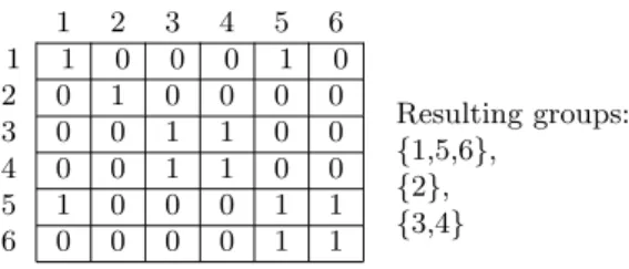
With the binary matrix BM , we then apply a transitive concept to group s-clusters. To illustrate this, in Figure 1, clusters 1, 5, and 6 can be grouped in one cluster since clusters 1 and 5 are similar, and clusters 5 and 6 are also similar (The other two clusters are {2} and {3,4}). This merging step requires O(n2) computation, which is similar to hierarchical clustering. However, the computation is conducted for n s-clusters instead of data objects. In addition, this transitive concept allows the arbitrary shape of clusters to be discovered.
3 Visualization with CDCS
Simply speaking, visualization in CDCS is implemented by transforming a cluster into a graphic line connected by 3D points. These three dimensions represent the attributes, attribute values and the percentages of an attribute value in the cluster. These lines can then be observed in 3D space through rotations. In the following, we first introduce the principle behind our visualization method; and then describe how it can help determine a proper clustering.
1 2 3 4 5 6
1 1 0 0 0 1 0
2 0 1 0 0 0 0
3 0 0 1 1 0 0
4 0 0 1 1 0 0
5 1 0 0 0 1 1
6 0 0 0 0 1 1
Resulting groups: {1,5,6},
{2}, {3,4}
Fig. 1.Binary similarity matrix (BM)
3.1 Principle of visualization
Ideally, each attribute Ai of a cluster Cxhas an obvious attribute value vi,ksuch that the probability of the attribute value in the cluster, P (Ai = vi,k|Cx), is maximum and close to 100%. Therefore, a cluster can be represented by these attribute values. Consider the following coordinate system where the X coordi- nate axis represents the attributes, the Y-axis represents attribute values corre- sponding to respective attributes, and the Z-axis represents the probability that an attribute value is in a cluster. Note that for different attributes, the Y-axis represents different attribute value sets. In this coordinate system, we can denote a cluster by a list of d 3D coordinates, (i, vi,k, P(vi,k|Cx)), i = 1, . . . , d, where d denotes the number of attributes in the data set. Connecting these d points, we get a graphic line in 3D. Different clusters can then be displayed in 3D space to observe their closeness.
This method, which presents only attribute values with the highest propor- tions, simplifies the visualization of a cluster. Through operations like rotation or up/down movement, users can then observe the closeness of s-clusters from various angles and decide whether or not they should be grouped in one clus- ter. Graphic presentation can convey more information than words can describe. Users can obtain reliable thresholds for clustering since the effects of various thresholds can be directly observed in the interface.
3.2 Building a coordinate system
To display a set of s-clusters in a space, we need to construct a coordinate system such that interference among lines (different s-clusters) can be minimized in order to observe closeness. The procedure is as follows. First, we examine the attribute value with the highest proportion for each cluster. Then, summarize the number of distinct attribute values for each attribute, and then sort them in increasing order. Attributes with the same number of distinct attribute values are further ordered by the lowest value of their proportions. The attribute with the least number of attribute values are arranged in the middle of the X-axis and others are put at two ends according to the order described above. In other words, if the attribute values with the highest proportion for all s-clusters are the same for some attribute Ak, this attribute will be arranged in the middle of the X-axis. The next two attributes are then arranged at the left and right of Ak.
After the locations of attributes on the X-axis are decided, the locations of the corresponding attribute values on the Y-axis are arranged accordingly. For each s-cluster, we examine the attribute value with the highest proportion for each attribute. If the attribute value has not been seen before, it is added to the
“presenting list” (initially empty) for that attribute. Each attribute value in the presenting list has a location as its order in the list. That is, not every attribute value has a location on the Y-axis. Only attribute values with the highest pro- portion for some clusters have corresponding locations on the Y-axis. Finally, we represent a s-cluster Ck by its d coordinates (Lx(i), Ly(vi,j), P (vi,j|Ck)) for i= 1, . . . , d, where the function Lx(i) returns the X-coordinate for attribute Ai, and Ly(v) returns the Y-coordinate for attribute value v.
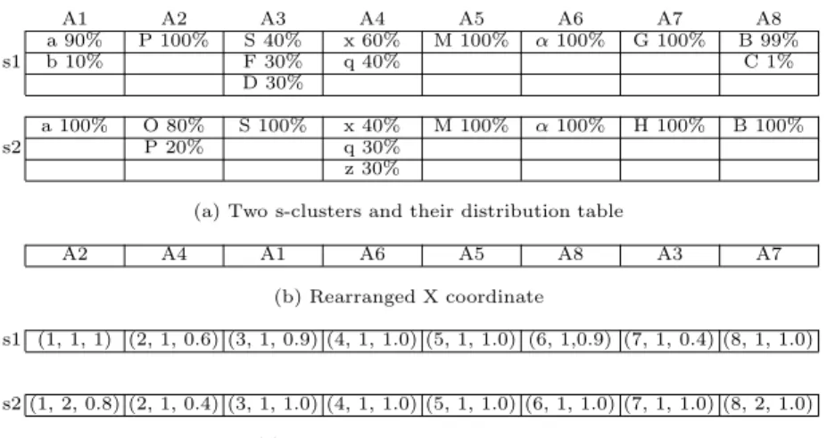
A1 A2 A3 A4 A5 A6 A7 A8
a 90% P 100% S 40% x 60% M 100% α100% G 100% B 99%
s1 b 10% F 30% q 40% C 1%
D 30%
a 100% O 80% S 100% x 40% M 100% α100% H 100% B 100%
s2 P 20% q 30%
z 30%
(a) Two s-clusters and their distribution table
A2 A4 A1 A6 A5 A8 A3 A7
(b) Rearranged X coordinate
s1 (1, 1, 1) (2, 1, 0.6) (3, 1, 0.9) (4, 1, 1.0) (5, 1, 1.0) (6, 1,0.9) (7, 1, 0.4) (8, 1, 1.0)
s2 (1, 2, 0.8) (2, 1, 0.4) (3, 1, 1.0) (4, 1, 1.0) (5, 1, 1.0) (6, 1, 1.0) (7, 1, 1.0) (8, 2, 1.0) (c) 3-D coordinates for s1 and s2
Fig. 2.Example of constructing a coordinate system
In Figure 2 for example, two s-clusters and their attribute distributions are shown in (a). Here, the number of distinct attribute values with the highest proportion is 1 for all attributes except for A2and A7. For these attributes, they are further ordered by the lowest proportion. Therefore, the order for these 8 attributes are A5, A6, A8, A1, A3, A4, A7, A2. With A5 as center, A6 and A8 are arranged to the left and right, respectively. The rearranged order of attributes is shown in Figure 2(b). Finally, we transform cluster s1, and then s2 into the coordinate system we build, as shown in Figure 2(c). Taking A2 for example, the presenting list includes P and O. Therefore, P gets a location 1 and O a location 2 at Y-axis. Similarly, G gets a location 1 and H a location 2 at Y-axis for A7.
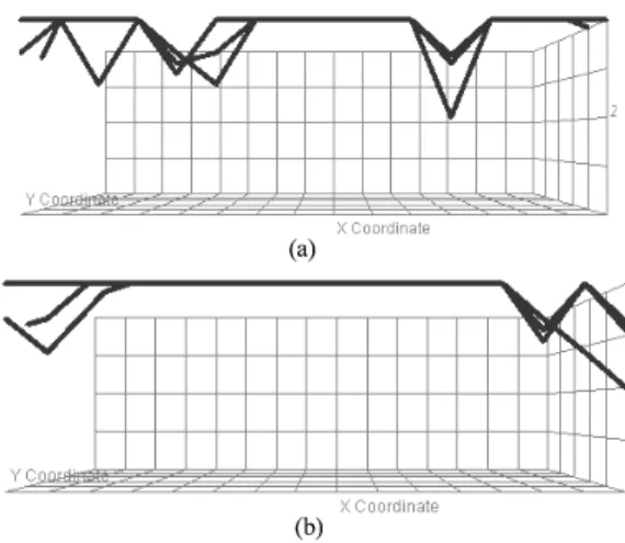
Figure 3 shows an example of three s-clusters displayed in one window before (a) and after (b) the attribute rearrangement. The thickness of lines reflects the size of the s-clusters. Comparing to the coordinate system without rearranging attributes, s-clusters are easier to observe in the new coordinate system since
common points are located at the center along the X-axis presenting a trunk for the displayed s-clusters. For dissimilar s-clusters, there will be a small number of common points, leading to a short trunk. This is an indicator whether the displayed clusters are similar and this concept will be used in the interactive analysis described next.
✁✄✂
☎✆✂
Fig. 3.Three s-clusters (a) before and (b) after attribute rearrangement.
3.3 Interactive visualization and analysis
The CDCS’s interface, as described above, is designed to display the merging result of s-clusters such that users know the effects of adjusting parameters. Instead of showing all s-clusters, our visualization tool displays only two groups from the merging result. More specifically, our visualization tool presents two groups in two windows for observing. The first window displays the group with the most number of s-clusters since this group is usually the most complicated case. The second window displays the group which contains the cluster pair with the lowest similarity. The coordinate systems for the two groups are conducted respectively.
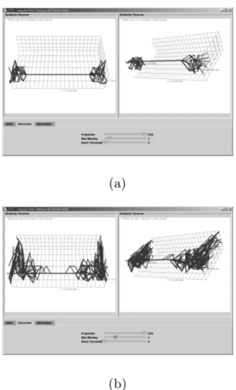
Figure 4 shows an example of the CDCS’s interface. The dataset used is the Mushroom database taken from UCI [1]. The number of s-clusters obtained from the first step is 106. The left window shows the group with the largest number of s-clusters, while the right window shows the group with the least similar s-cluster pair. The number of s-clusters for these groups are 16 and 13, respectively, as shown at the top of the windows. Below these two windows, three sliders are used to control the parameters for group merging and visualization. The first two sliders denote the parameters p′ and e′ used to control similarity threshold
g′. The third slider is used for noise control in the visualization so that small s-clusters can be omitted to highlight the visualization of larger s-clusters. Each time the slider is moved, the merging result is computed and updated in the windows. Users can also lock one of the windows for comparison with different threshold.
(a)
(b)
Fig. 4.Visualization of the mushroom dataset (a) a strict threshold (b) a mild threshold
A typical process for interactive visualization analysis with CDCS is as fol- lows. We start from a strict threshold g′ such that the displayed groups are compact; and then relax the similarity threshold until the displayed groups are too complex. A compact group usually contains a long trunk such that all s- clusters in the group have same values and high proportions for these attributes. A complex group, on the other hand, presents short trunk and contains different values for many attributes. For example, both groups displayed in Figure 4(a) have obvious trunks which are composed of sixteen common points (or attribute values). For a total of 22 attributes, 70% of the attributes have the common values and proportions for all s-clusters in the group. Furthermore, the propor- tions of these attribute values are very high. Through rotation, we also find that the highest proportion of the attributes outside the trunk is similarly low for all s-clusters. This implies that these attributes are not common features for these
s-clusters. Therefore, we could say both these groups are very compact since these groups are composed of s-clusters that are very similar.
If we relax the parameter e′from 2 to 5, the largest group and the group with least similar s-clusters are the same group which contains 46 s-clusters, as shown in Figure 4(b). For this merging threshold, there is no obvious trunk for this group and some of the highest proportions outside the trunk are relatively high while some are relatively low. In other words, there are no common features for these s-clusters, and this merge threshold is too relaxed since different s-clusters are put in the same group. Therefore, the merging threshold in Figure 4(a) is better than the one in Figure 4(b).
In summary, whether the s-clusters in a group are similar is based on users’ viewpoints on the obvious trunk. As the merging threshold is relaxed, more s-clusters are grouped together and the trunks of both windows get shorter. Sometimes, we may reach a stage where the merge result is the same no matter how the parameters are adjusted. This may be an indicator of a suitable cluster- ing result. However, it depends on how we view these clusters since there may be several such stages.
4 Experiments
We presents an experimental evaluation of CDCS on five real-life data sets from UCI machine learning repository [1] and compares its result with AutoClass [2] and k-mode [4]. The number of clusters required for k-mode is obtained from the clustering result of CDCS. To study the effect due to the order of input data, each dataset is randomly ordered to create four test data sets for CDCS. Four users are involved in the visualization analysis to decide a proper grouping criteria.
The five data sets used are Mushroom, Soybean-small, Soybean-large, Zoo dataset and Congress Voting which have been used for other clustering algo- rithms. Table 1 records the number of clusters and the clustering accuracy for the 5 data sets. As shown in the last row, CDCS has better clustering accuracy than the other two algorithms. CDCS is better than K-mode in each experiment given the same number of clusters. However, the number of clusters found by CDCS is more than that found by AutoClass, especially for the last two data sets. The main reason for this phenomenon is that CDCS reflects users’ view on the degree of intracluster cohesion. Various clustering results, say 9 clusters and 10 clusters, can not be observed in this visualization method. In general, CDCS has better intracluster cohesion for all data sets, while AutoClass has better cluster separation (smaller intercluster similarity) on the whole.
5 Conclusion
In this paper, we introduced a novel approach for clustering categorical data based on two ideas. First, a classification-based concept is incorporated in the computation of object similarity to clusters; and second, a visualization method
# of clusters Accuracy AutoClass CDCS AutoClass K-mode CDCS
Mushroom 22 21 0.9990 0.9326 0.996
22 attributes 18 23 0.9931 0.9475 1.0
8124 data 17 23 0.9763 0.9429 0.996
2 labels 19 22 0.9901 0.9468 0.996
Zoo 7 7 0.9306 0.8634 0.9306
16 attributes 7 8 0.9306 0.8614 0.9306
101 data 7 8 0.9306 0.8644 0.9306
7 labels 7 9 0.9207 0.8832 0.9603
Soybean-small 5 6 1.0 0.9659 0.9787
21 attributes 5 5 1.0 0.9361 0.9787
47 data 4 5 1.0 0.9417 0.9574
4 labels 6 7 1.0 0.9851 1.0
Soybean-large 15 24 0.664 0.6351 0.7500 35 attributes 5 28 0.361 0.6983 0.7480
307 data 5 23 0.3224 0.6716 0.7335
19 labels 5 21 0.3876 0.6433 0.7325
Voting 5 24 0.8965 0.9260 0.9858
16 attributes 5 28 0.8942 0.9255 0.9937
435 data 5 26 0.8804 0.9312 0.9860
2 labels 5 26 0.9034 0.9308 0.9364
Average 0.8490 0.8716 0.9260
Table 1.Number of clusters and clustering accuracy for three algorithms
is devised for presenting categorical data in a 3-D space. Through interactive visualization interface, users can easily decide a proper parameter setting. From the experiments, we conclude that CDCS performs quite well compared to state- of-the-art clustering algorithms. Meanwhile, CDCS handles successfully data sets with significant differences in the sizes of clusters. In addition, the adoption of naive-Bayes classification makes CDCS’s clustering results much more easily interpreted for conceptual clustering.
Acknowledgements
This work is sponsored by National Science Council, Taiwan under grant NSC92- 2213-E-008-028.
References
1. C.L. Blake and C.J. Merz. UCI repository of machine learning databases. [http://www.cs.uci.edu/∼mlearn/MLRepository.html]. Irvine, CA., 1998.
2. P. Cheeseman and J. Stutz. Bayesian classification (autoclass): Theory and results. In Proceedings of Advances in Knowledge Discovery and Data Mining, pages 153– 180, 1996.
3. S. Guha, R. Rastogi, and K. Shim. ROCK: a robust clustering algorithm for cate- gorical attributes. Information Systems, 25:345–366, 2000.
4. Z. Huang. Extensions to the k-means algorithm for clustering large data sets with categorical values. Data Mining and Knowledge Discovery, 2:283–304, 1998. 5. T. M. Mitchell. Machine Learning. McGraw Hill, 1997.
6. J. T. To and R. C. Gonzalez. Pattern Recognition Principles. Addison-Wesley Publishing Company, 1974.