Lecture Note
Exotic Superconductivity
Department of Physics, University of Illinois at Urbana-Champaign
Anthony J. Leggett
(Received 18:00, 2 March 2012)
These are the lecture notes for a series of lectures “Exotic Superconductivity” done at the Graduate School of Science of The University of Tokyo, Japan, in May-June, 2011. These lectures are an introduction to those superconductors, all discovered since the 1970s, which do not appear to be well described by the traditional BCS theory. While the main emphasis will be on the most spectacular member of this class, the cuprates, I shall also discuss briefly the heavy fermion, organic, ruthenate and ferropnictide superconductors as well as superfluid 3He for reference. I shall try to provide a general framework for the analysis of all-electronic superconductivity (i.e. that in which the Cooper pairing is induced wholly or mainly by the repulsive Coulomb interaction).
These lecture notes were written by the following graduate students at The Univer- sity of Tokyo: Haruki Watanabe (UC Berkeley from Aug. 2011, Lec. 4, 7, 8), Hakuto Suzuki (Lec. 5, 6), Yuya Tanizaki (Lec. 1, 4, 6), Masaru Hongo (Lec. 2, 3), Kota Masuda (Lec. 1, 2, 3), and Shimpei Endo (Lec. 1, 5, 7, 8). We would like to thank Profs. Hiroshi Fukuyama and Masahito Ueda for the organization of the lecture series as well for the critical reading of these notes. We also thank Office of Communication and Office of Inter- nationalization Planning at the Graduate School of Science, and Office of Student Affairs at Physics Department of The University of Tokyo for their supports. The lectures were hosted as the Sir Anthony James Leggett Visit Program 2011-2013, financially supported by the JSPS Award for Eminent Scientists (FY2011-2013).
Slides and videos of the lectures are available at UT OpenCourseWare: http://ocw.u-tokyo.ac.jp/eng_courselist/828.html
Contents
Lec. 1 Reminders of the BCS theory 10
1.1 Basic model . . . 10
1.2 BCS theory at T = 0 . . . 11
1.2.1 BCS wave function . . . 11
1.2.2 Alternative form of the BCS wave function . . . 12
1.2.3 Pair wave function . . . 13
1.2.4 Quantitative development of the BCS theory . . . 15
1.3 BCS theory at finite temperature . . . 18
1.3.1 Derivation of the gap equation . . . 18
1.3.2 Fk at finite temperature . . . 20
1.3.3 hnki at finite temperature . . . 20
1.3.4 Properties of the BCS gap equation . . . 20
1.3.5 Properties of the Fock term . . . 23
1.3.6 Pair wave function . . . 23
1.4 Generalization of the BCS theory . . . 25
Lec. 2 Superfluid 3He: basic description 28 2.1 Introduction . . . 28
2.2 Landau Fermi liquid theory . . . 29
2.3 Effects of (spin) molecular field in 3He . . . 31
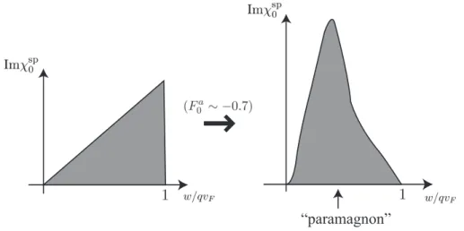
2.3.1 Enhanced low-energy spin fluctuations . . . 31
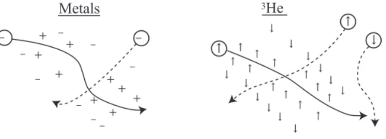
2.3.2 Coupling of atomic spins through the exchange of virtual paramagnons 32 2.3.3 Pairing interaction in liquid 3He . . . 32
2.4 Anisotropic spin-singlet pairing (for orientation only) . . . 33
2.5 Digression: macroscopic angular momentum problem . . . 34
2.6 Spin-triplet pairing . . . 35
2.6.1 Equal spin pairing (ESP) state . . . 36
2.6.2 General case . . . 36
2.6.3 d-vector (unitary states) . . . 37
2.7 Ginzburg–Landau theory . . . 38
2.7.1 Spin-singlet case . . . 38
2.7.2 Spin-triplet case . . . 39
A. J. Leggett
Lec. 3 Superfluid 3He (continued) 42
3.1 Experimental phases of liquid3He . . . 42
3.2 Nature of the order parameter of different phases . . . 43
3.2.1 A phase . . . 43
3.2.2 A1 phase . . . 44
3.2.3 B phase: naive identification . . . 45
3.3 Why A phase? . . . 45
3.3.1 Generalized Ginzburg–Landau approach . . . 46
3.3.2 Spin fluctuation feedback . . . 48
3.4 NMR in the new phase . . . 49
3.5 What can be inferred from the sum rules? . . . 50
3.6 Spontaneously broken spin-orbit symmetry . . . 51
3.7 Microscopic spin dynamics (schematic) . . . 54
3.8 Illustration of NMR behavior: A phase longitudinal resonance . . . 55
3.9 Digression: possibility of the “fragmented” state . . . 55
3.10 Superfluid 3He: supercurrents, textures, and defects . . . 57
3.10.1 Supercurrents . . . 57
3.10.2 Mermin–Ho vortex and topological singularities . . . 58
Lec. 4 Definition and diagnostics of “exotic” superconductivity 61 4.1 Diagnostics of the non-phonon mechanism . . . 62
4.1.1 Absence of isotope effect . . . 62
4.1.2 Absence of phonon structure in tunneling I-V characteristics . . . . 64
4.2 General properties of the order parameter . . . 65
4.2.1 Definition of the order parameter . . . 65
4.2.2 Order parameter in a crystal . . . 67
4.3 Diagnostics of the symmetry of the order parameter . . . 69
4.3.1 Diagnostics of the spin state . . . 69
4.3.2 Diagnostics of the orbital state . . . 71
4.3.3 Effect of impurities . . . 73
4.4 Addendum: the effect of spin-orbit coupling . . . 74
Lec. 5 Non-cuprate exotic superconductivity 77 5.1 Alkali fullerides . . . 77
5.1.1 Structure . . . 77
5.1.2 Fullerene crystals . . . 77
5.1.3 Alkali fullerides . . . 78
5.1.4 Superconducting state . . . 79
5.2 Organics . . . 80
5.2.1 Normal state . . . 80
5.2.2 Superconducting state . . . 81
A. J. Leggett
5.3 Heavy fermions . . . 82
5.3.1 Normal-state behavior . . . 82
5.3.2 Superconducting phase . . . 84
5.4 Strontium ruthenate: Sr2RuO4 . . . 86
5.4.1 History . . . 86
5.4.2 Experimental properties of Sr2RuO4 . . . 87
5.5 Ferropnictides . . . 91
5.5.1 Composition . . . 91
5.5.2 Structure (1111 compounds) . . . 91
5.5.3 Phase diagram . . . 92
5.5.4 Experimental properties (normal state) . . . 92
5.5.5 Band structure . . . 93
5.5.6 Superconductivity . . . 94
5.5.7 Experimental properties (superconducting state) . . . 94
5.5.8 Pairing state . . . 95
Lec. 6 Cuprates: generalities, and normal state properties 98 6.1 Basic chemical properties . . . 98
6.1.1 Composition . . . 98
6.1.2 Structure . . . 98
6.2 Doping . . . 99
6.3 Construction of phase diagram . . . 101
6.4 Determinants of Tc . . . 103
6.5 Other remarks: carrier density and list of cuprate superconductors . . . 104
6.6 Experimental properties of the normal state: general discussion . . . 105
6.7 Experimental properties at the optimal doping . . . 106
6.7.1 Electronic specific heat . . . 106
6.7.2 Magnetic properties . . . 106
6.7.3 Transport . . . 106
6.7.4 Spectroscopic probes: Fermi surface . . . 108
6.7.5 Results of ARPES experiments at the optimal doping . . . 109
6.7.6 Neutron scattering . . . 110
6.7.7 Optics (ab-plane) . . . 110
6.8 Experimental properties at the underdoped regime . . . 111
6.8.1 Pseudogap . . . 111
6.8.2 ARPES in the pseudogap regime: the puzzle of the Fermi surface . 113 Lec. 7 Cuprates: superconducting state properties 117 7.1 Experimental properties . . . 117
7.1.1 Structural and elastic properties and electron density distribution . 117 7.1.2 Macroscopic electromagnetic properties . . . 117
A. J. Leggett
7.1.3 Specific heat and condensation energy . . . 118
7.1.4 NMR . . . 118
7.1.5 Penetration depth . . . 118
7.1.6 AC conductivity . . . 120
7.1.7 Thermal conductivity . . . 121
7.1.8 Tunneling . . . 121
7.1.9 ARPES . . . 122
7.1.10 Neutron scattering (YBCO, LSCO, and Bi-2212) . . . 123
7.1.11 Optics . . . 123
7.1.12 Electron energy loss spectroscopy (EELS) . . . 125
7.2 What do we know for sure about superconductivity in the cuprates? . . . . 125
7.3 Symmetry of the order parameter (gap) . . . 128
7.4 Josephson experiment in cuprate (and other exotic) superconductors . . . . 131
7.5 What is a “satisfactory” theory of the high-Tc superconductivity in the cuprates? . . . 133
Lec. 8 Exotic superconductivity: discussion 136 8.1 Common properties of all exotic superconductors . . . 136
8.2 Phenomenology of superconductivity . . . 137
8.2.1 Meissner effect . . . 138
8.2.2 Persistent current . . . 138
8.2.3 Summary . . . 138
8.3 What else do exotic superconductors have in common? . . . 140
8.4 Theoretical approaches (mostly for the cuprates) . . . 140
8.5 Which energy is saved in the superconducting phase transition? . . . 143
8.5.1 Virial theorem . . . 144
8.5.2 Energy consideration in “all-electronic” superconductors . . . 147
8.5.3 Eliashberg vs. Overscreening . . . 148
8.5.4 Role of two-dimensionality . . . 149
8.5.5 Constraints on the Coulomb saved at small q . . . 150
8.5.6 Mid-infrared optical and EELS spectra of the cuprates . . . 152
8.6 How can we realize room temperature superconductors? . . . 154
A. J. Leggett
List of Symbols
Symbol Meaning
Page where defined /introduced
|↑i spin up state 11
|↓i spin down state 11
|00i state with (k ↑,−k ↓) states unoccupied 12
|11i state with (k ↑,−k ↓) states occupied 12
a, a† creation/annihilation operators 10
αkσ, α†kσ creation/annihilation operators for quasi- particles (not for bare particles)
33
A(k, ε) spectral function 108
ck coefficient of the pair wave function 36
CV specific heat 28
d d-vector 38
dn/dε density of states of both spins at the Fermi surface
21 dx2−y2 most popular symmetry of cupurate order
parameter
130
Ds spin diffusion constant 28
e electron charge 26
E0 ground state energy of the interacting sys- tem
29
Ek BCS excitation energy 16
EBP energy of the broken-pair state 18
EEP energy of the excited-pair state 18
EGP energy of the ground-pair state 18
EJ Josephson coupling energy 131
F free energy 39
F (k) relative wave function of the Cooper pair 23 f (pp′σσ′) Landau interaction function 29
F (ω) phonon density of states 63
Fℓs, Fℓa Landau parameters 30
gD nuclear dipole coupling constant 52
Hc1 lower critical field 81
Hc2 upper critical field 81
HˆD nuclear dipole energy 51
Hext external magnetic field 50
k wave vector 10
kB Boltzmann’s constant 21
A. J. Leggett
Symbol Meaning
Page where defined /introduced
kF Fermi wave number 10
Ks Knight shift 73
ℓˆ direction of relative orbital angular mo- mentum of pairs in the A phase
43
ℓel mean free paths of electrons 121
ℓph mean free paths of phonons 121
L orbital angular momentum 45
L(ω) loss function 110
m mass of atoms/electrons 10
m∗ effective mass of atoms/electrons 30
n particle density 13
N (0) density of states of one spin at the Fermi surface (≡ 1/2(dn/dε))
21
NCooper number of the Cooper pairs 24
Ns density of states 72
p doping (of cuprates) 101
pF Fermi momentum 29
qTF Thomas-Fermi wave number 26
Q pseudo-Bragg vector 142
R center-of-mass coordinate 72
R(ω) optical reflectivity 110
S total spin 31
T∗ crossover line (in the phase diagram of cuprates)
102
T1 nuclear spin relaxation time 73
Tc critical temperature 20
TCurie Curie temperature 85
TN N`eel temperature 85
uk coefficient in the BCS wave function 12
vF Fermi velocity 25
vk coefficient in the BCS wave function 12
vs superfluid velocity 57
αI isotope exponent 63
α(ω) phonon coupling function 63
β 1/kBT 19
γ coefficient of the linear term in the specific heat
87 Γl relaxation rate of ℓ-symmetry distortion 74
A. J. Leggett
Symbol Meaning
Page where defined /introduced ΓU relaxation rate of the T -reversal operator 74
δn deviation of (quasi)particle occupation number from the normal-state value
29
∆k BCS gap parameter 16
εc cutoff energy in the BCS model 21
εF Fermi energy 10
εk kinetic energy relative to the Fermi energy 10
η viscosity 28
ΘD Debye temperature 63
κ thermal conductivity 28
κ0 static bulk modulus of the non-
interactiong Fermi gas
26
λ London penetration depth 79
µ chemical potential 10
µ∗ Coulomb pseudopotential 63
µB Bohr magneton 52
µn nuclear magnetic moment 50
ξ healing length 24
ξPR pair radius 14
ξab in-plane Ginzburg-Landau healing length 117
ξk kinetic energy 10
ξc c-axis Ginzburg-Landau healing length 117
ρ(T ) resistivity 80
ρ1, ρ2 single-particle/two-particle density matri- ces
65
ρk single-particle density 18
ρs superfluid density 57
σ(ω) AC conductivity 107
τ relaxation time 107
φ(k) phase of the condensate wave function 13 φ(r1σ1; r2σ2) pseudo-molecular wave function in the
BCS problem
11 Φ0 (superconducting) flux quantum (≡ h/2e) 131
χ Pauli spin susceptibility 28
χsp spin response 31
Ψ( ˆn) Ginzburg-Landau order parameter 38
Ψ(r1σ1, r2σ2· · · rNσN) many-body wave function 11
ωD Debye frequency 21
A. J. Leggett
Symbol Meaning
Page where defined /introduced ωe some characteristic frequency of the order
of the plasma frequency
153
ωp plasma frequency 153
ωph frequency of the longitudinal sound waves (phonons)
64
ωres response frequency 50
ωSF AF fluctuation frequency 142
Lec. 1 Reminders of the BCS
theory
First we give a brief review of the theory of conventional superconductors, namely the BCS theory. In this section, we start with the singlet pairing case to describe the basic physics of the superconductivity.
1.1 Basic model
Just as in the original BCS theory, we consider here the Sommerfeld model for sim- plicity: we consider N spin-1/2 fermions in a free space. We assume N to be sufficiently large and even. For such a system, the kinetic energy for a free particle is
εk ≡ ξk− µ(T ), (1.1)
where ξk = k
2
2m, and µ(T ) is the chemical potential of the system. We note here that µ(T ) can be regarded as a constant1, and it is equal to the Fermi energy
µ(T ) = εF = k
2F
2m. (1.2)
We assume that the fermions are interacting via an attractive potential, so that the interaction part can be represented as
V =ˆ 1 2
∑
p,p′,q σ,σ′
Vp,p′,q a†p+q
2,σ
a†p′−q 2,σ
′ap′+q
2,σ
′ap−q
2,σ. (1.3)
We do not discuss here the origin of this interaction (we will present the discussion in Sec. 1.3.4), but rather try to see how the system behaves under such an attractive inter- action.
1In fact, the temperature in question is very small in discussing the BCS theory, and thus the tem- perature dependence of the chemical potential due to the Fermi statistics is negligible. In addition, the effect of the superconducting phase transition to the chemical potential is very small in the BCS theory.
A. J. Leggett LEC. 1. REMINDERS OF THE BCS THEORY
1.2 BCS theory at T = 0
1.2.1 BCS wave function
Under an attractive interaction, the Fermi system forms Cooper pairs and they undergo Bose-Einstein condensation. When the Bose-Einstein condensation occurs, a macroscopic number of bosons occupy the same state. Therefore, as a fundamental assumption, we think that all the pairs of fermions occupy the same pair wave function φ:
ΨN = Ψ(r1σ1, r2σ2...rNσN) = A[φ(r1σ1; r2σ2)φ(r3σ3; r4σ4) · · · φ(rN −1σN −1; rNσN)], (1.4) where A is the antisymmetrizer. For now, we restrict our attention to the case where pairs are formed in the spin-singlet, s-wave orbital angular momentum state, and the center of mass of the pairs is at rest. Then the pair wave function φ becomes
φ(r1σ1; r2σ2) = √1 2
[|↑i1|↓i2− |↓i1|↑i2
]φ(r1− r2), (1.5) where φ(r) = φ(−r). If we define the Fourier transform χ(k) by
φ(r) =∑
k
χ(k)eikr, (1.6)
then we find
φ(r1σ1; r2σ2) = √1 2
[|↑i1|↓i2− |↓i1|↑i2
]∑
k
χ(k)eik(r1−r2)
=∑
k
χ(k)√ 2
[|k ↑i1|−k ↓i2− |k ↓i1|−k ↑i2
]
=∑
k
χ(k)√ 2
[|k ↑i1|−k ↓i2− |−k ↓i1|k ↑i2
]
=∑
k
χ(k)a†k↑a†−k↓|vaci ,
(1.7)
where we have used χ(k) = χ(−k) in the second last line. Therefore, if we define Ω†≡∑
k
χ(k)a†k↑a†−k↓, (1.8)
the N -body wave function defined in Eq. (1.4) is rewritten as ΨN = (Ω†)N/2|vaci =[ ∑
k
χ(k)a†k↑a†−k↓]N/2|vaci . (1.9) Note that this is automatically an eigenstate of ˆN . We also note that the normal ground state is a special case of this form of the wave function, since we can see
ΨnormN = ∏
k<kF
a†k↑a†−k↓|vaci =( ∑
k<kF
a†k↑a†−k↓)N/2|vaci (1.10) from the Fermi statistics, and the final expression corresponds to the BCS wave function with χ(k) = θ(kF − |k|).
A. J. Leggett LEC. 1. REMINDERS OF THE BCS THEORY
1.2.2 Alternative form of the BCS wave function
In the previous subsection, we have obtained the many-body wave function which au- tomatically conserves the number of particles N . In principle, we can minimize the free energy with this class of wave functions and study the thermodynamic properties of the system, but it is a tough work. Therefore, we replace the wave function in the following way:
(Ω†)N/2 → exp Ω†≡
∞
∑
N/2=0
1 (N/2)!(Ω
†)N/2, (1.11)
and we try to minimize ˆH − µ ˆN instead of ˆH. Hence, up to the normalization, the wave function becomes
Ψ ∝ exp (
∑
k
χ(k)a†k,↑a†−k,↓ )
|vaci =∏
k
exp(χ(k)a†k,↑a†−k,↓)|vaci. (1.12)
Since (a†k,↑a†−k,↓)2 = 0 due to the Fermi statistics, it reads Ψ ∝∏
k
(1 + χ(k)a†k,↑a†−k,↓)|vaci. (1.13) To make clear the physical meanings of the following calculations, we go over to the representation in terms of occupation spaces of k ↑, −k ↓; let |00ik be the corresponding vacuum, and define
|10ik= a†k,↑|00ik, |01ik = a†−k,↓|00ik, and |11ik= a†k,↑a
†
−k,↓|00ik. (1.14) Then the wave function Ψ can be represented as
Ψ =∏
k
Φk, (1.15)
where
Φk∝ |00ik+ χk|11ik. (1.16)
To satisfy the normalization condition, multiply by the factor 1/√1 + |χk|2, and then we obtain
Φk= uk|00ik+ vk|11ik, (1.17) with uk = 1
√1 + |χk|2
and vk = χk
√1 + |χk|2
. Thus, we have obtained the general form of the BCS wave function as
ΨBCS =∏
k
(uk|00ik+ vk|11ik) =∏
k
(uk+ vka†k,↑a†−k,↓)|vaci, (1.18)
which does not conserve the number of particles. The normal ground state corresponds to a special case of this wave function, which can be obtained by setting uk = 0, vk = 1
A. J. Leggett LEC. 1. REMINDERS OF THE BCS THEORY
We should make some remarks on the BCS wave function and the above derivation. At first we should notice that this is the very general result for the spin-singlet paring systems in the sense that the coefficients uk and vk can depend on the direction of the momentum k. Since the phase transformation (uk, vk) → eiφk(uk, vk) has no physical effect, we can choose all uk to be real.
As a consequence of the number conservation, we can find that the transformation vk → eiφvk, where φ is independent of k, has no physical effects either. To see this, let us define
ΨBCS(φ) =∏
k
(uk+ eiφvka†k,↑a†−k,↓)|vaci. (1.19)
From this, we can easily check that ∂
∂φΨBCS(φ) = i ˆN ΨBCS(φ). When we define
h ˆAiφ = Ψ†BCS(φ) ˆAΨBCS(φ), (1.20)
where ˆA is a physical (hence number-conserving) operator, we can see that this expectation value does not depend on the phase φ:
d
dφh ˆAiφ = iΨ
†
BCS(φ)[ ˆA, ˆN ]ΨBCS(φ) = 0. (1.21)
We can, therefore, construct the number-conserving many body wave function: ΨN = 1
2π
∫ 2π 0
dφΨBCS(φ)e−iφN2 . (1.22)
1.2.3 Pair wave function
Let us discuss the relative wave function of a Cooper pair. In the BCS theory , the pair wave function at T = 0 is expressed as
Fk= ukvk, (1.23)
or as its Fourier transformation F (r) =∑kFkeikr.
The physical meaning of the pair wave function becomes clearer if we evaluate the expectation value of the potential energy h ˆV i:
h ˆV i = 12∑
pp′q σσ′
Vpp′qha†p+q/2,σa†p′−q/2,σ′ap′+q/2,σ′ap−q/2,σi. (1.24)
For the BCS wave function, only three types of terms contribute to the expectation value: the Hartree term (q = 0), the Fock term (σ = σ′, p = p′), and the pairing term (p + q2 = −(p′ −q2) , σ = −σ′). The Hartree term can be evaluated as
h ˆV iHartree = 1 2
∑
pp′ σσ′
Vpp′0hnpσnp′σ′i. (1.25)
A. J. Leggett LEC. 1. REMINDERS OF THE BCS THEORY
Especially, for the case of the local potential V = V (r), the Hartree term h ˆV iHartree becomes a constant 12V (q = 0)h ˆN2i.
The Fock term, corresponding to σ = σ′, p = p′, is given by h ˆV iFock = −1
2
∑
pqσ
Vppqhnp+q/2,σnp−q/2,σi = −
1 2
∑
pq
|vp+q/2|2|vp−q/2|2. (1.26) The last equality is a consequence of the uncorrelated nature of the BCS wave function, and it can be easily checked by a direct calculation.
Finally we evaluate the pairing term. For convenience, we introduce the following variables: k = p + q/2 and k′ = p − q/2. Then, we have
h ˆV ipair = 12∑
k,k′
Vkk′ha†k′,σa−k† ′,−σ′a−k,−σak,σi, (1.27) where Vkk′ = Vk+q/2,k′−q/2,k−k′, which is V (k −k′) for a local potential V (r). Again using the factorizable nature of the BCS wave function except for the O(1/N) contributions, this reduces to
h ˆV ipair = 12 ∑
kk′σ
Vkk′ha†k′,σa†−k′,−σ′iha−k,−σak,σi
= 1 2
∑
kk′σ
Vkk′ha†k′↑a†−k′↓iha−k↓ak↑i.
(1.28)
At last, we have used the spin-singlet nature of the BCS wave function. We can find by an explicit calculation that
ha−k,↓ak,↑i = u∗kvkh00|a−k,↓ak↑|11i = ukvk = Fk. (1.29) Similarly, we can obtain that ha†k,↑a
†
−k,↓i = ukvk∗ = Fk∗. Hence, the pairing interaction is h ˆV ipair=∑
kk′
Vkk′FkFk∗′. (1.30) In the case of a local potential V (r), we can rewrite this in terms of the Fourier component of F (r):
h ˆV ipair =
∫
d3rV (r)|F (r)|2. (1.31)
The comparison of this result with the interaction between two particles in free space h ˆV i =∫ d3rV (r)|Ψ(r)|2 tells us that F (r) essentially works as the relative wave function Ψ(r) of the pair in the superfluid Fermi system. It is a much simpler quantity to deal with than the quantity φ(r), which appears in the N -conserving formalism.
We do not yet know the specific form of u’s and v’s in the ground state, and we cannot calculate the form of F (r) now. We, however, anticipate that it will be bound in relative space and that we will be able to define a “pair radius” by the quantity
ξPR2 = ∫ d
3r|F (r)|2|r|2
∫ d3r|F (r)|2 . (1.32)
It cannot be too strongly emphasized that everything above is very general and true
A. J. Leggett LEC. 1. REMINDERS OF THE BCS THEORY
1.2.4 Quantitative development of the BCS theory
We consider a fully condensed BCS state described by the N -nonconserving wave func- tion:
Ψ =∏
k
Φk, Φk≡ uk|00ik+ vk|11ik. (1.33) From the normalization condition, uk and vk should satisfy the following relation:
|uk|2+ |vk|2 = 1. (1.34)
The values of uk, vk are determined by minimizing the free energy:
h ˆHi = h ˆT − µ ˆN + ˆV i. (1.35) Let us neglect2 the Fock term in h ˆV i unless mentioned otherwise (we have already seen below Eq. (1.25) that the Hartree term contributes only a constant for the local potential case). Then, the contribution of h ˆV i comes only from the pairing terms
h ˆV i =∑
k,k′
Vkk′FkFk∗′, Fk ≡ ukvk. (1.36)
Here, Vkk′ is a matrix element for the process where fermions change the state from (k ↓, −k ↑) to (k′ ↑, k′ ↓). Let us consider the term
T − µ ˆˆ N =∑
k,σ
ˆ
nkσ(ξk− µ) ≡
∑
k,σ
ˆ
nkσεk. (1.37)
It is clear that |00ik and |11ik are eigenstates of ˆnkσ with their eigenvalues 0 and 2, respectively. Taking the sum of the spins, we find
h ˆT − µ ˆN i = 2∑
k
εk|vk|2, (1.38)
and therefore we obtain
h ˆHi = 2∑
k
εk|vk|2+∑
k,k′
Vkk′(ukvk)(uk′vk∗′). (1.39)
This h ˆHi must be minimized under the constraint |uk|2+ |vk|2 = 1. We introduce a pretty way of visualizing the problem. Let us put
uk(= real) = cosθk
2, vk= sin θk
2 expiφk, (1.40)
and rewrite the Hamiltonian as h ˆHi =∑
k
(−εkcosθk) + 14∑
k,k′
Vkk′sinθksinθk′cos(φk− φk′) +∑
k
εk. (1.41)
2In fact, we can shot that the Fock term have little effects. We will consider this effect later.
A. J. Leggett LEC. 1. REMINDERS OF THE BCS THEORY
The last term is a mere constant, so that we can neglect it. Next, we introduce the Anderson pseudospin representation of the BCS Hamiltonian. We introduce a unit vector σk with its polar angle given by (θk, φk):
sinθkcosφk = σxk, sinθksinφk = σyk, cosθk= σzk.
(1.42)
With this representation, the expectation value is rewritten as h ˆHi = −∑
k
εkσzk+1 4
∑
k,k′
Vkk′σk⊥· σk′⊥ = −
∑
k
σk· Hk, (1.43)
where σk⊥ is the xy-component of σk, and the pseudo-magnetic field Hk is defined as
Hk ≡ −εkz − ∆ˆ k, (1.44)
∆k ≡ −
1 2
∑
k′
Vkk′σk′⊥. (1.45)
Thus, the z-component of Hk gives the kinetic energy, while the xy-component is the potential energy (see Fig. 1.1).
It is actually very convenient to represent ∆k and σk⊥ as complex numbers ∆k ≡
∆kx+ i∆ky, σk⊥ ≡ σkx+ iσky rather than representing them as vectors. Evidently, the magnitude of the field Hk is
|Hk| = (ε2k+ |∆k|2)1/2 ≡ Ek, (1.46) In the ground state the spin σk lies along the field Hk, giving an energy −Ek. If the spin is reversed, this costs 2Ek (not Ek!). This reversal corresponds to
θk → π − θk, φk → φk+ π, (1.47)
Fig. 1.1. Schematic illustration of the vectors Hk and σk. At equilibrium, Hk and σk should point the same direction.
A. J. Leggett LEC. 1. REMINDERS OF THE BCS THEORY
and
uk→ sin
θk
2exp(−iφk) = v
∗ k,
vk→ −cos
θk
2 = −uk.
(1.48)
Therefore, the wave function of the excited state generated in this way is
ΨEPk = vk∗|00i − uk|11i , (1.49) We can easily verify that this excited state is orthogonal to the ground state Φk ≡
uk|00i + vk|11i (remember we take uk to be real).
Let us derive the BCS gap equation. Since the vector σk must point along the field Hk in the ground state, this gives a set of self-consistent conditions for ∆k; since σk′⊥ =
−∆k′/Ek′, we have
∆k= −
∑
k′
Vkk′
∆k′
2Ek′
. (1.50)
This is the BCS gap equation. Note that the above derivation is quite general. In particular, we have never assumed the s-wave state (though we did assume the spin- singlet pairing).
Let us also introduce an alternative derivation of the BCS gap equation. We simply parametrize uk and vk by ∆k and Ek as
uk≡
Ek+ εk
√|∆k|2+ (Ek+ εk)2, (1.51) vk ≡
∆k
√|∆k|2 + (Ek+ εk)2. (1.52) This clearly satisfies the normalization condition |uk|2+ |vk|2 = 1, and gives
|uk|2 = 12 [
1 + εk Ek
]
, |vk|2 = 12 [
1 −Eεk
k
]
, ukvk= ∆k 2Ek
. (1.53)
The BCS ground state energy can therefore be written in the form h ˆHi =∑
k
εk
(
1 − Eεk
k
)
+∑
kk′
Vkk′
∆k
2Ek
∆∗k′
2Ek′
. (1.54)
Here, ∆k for each k are independent variational parameters. By using ∂Ek/∂∆k =
∆∗k/Ek, we find
ε2k Ek3
[
∆∗k−∑
k′
Vkk′
∆∗k′
2Ek′
]
= 0, (1.55)
so that we again obtain the standard gap equation.
A. J. Leggett LEC. 1. REMINDERS OF THE BCS THEORY
(a) (b)
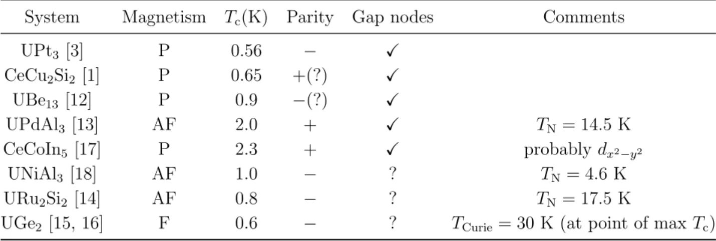
Fig. 1.2. (a) The number distribution and (b) the pair wave function for the BCS ground state.
For the s-wave state, ∆k is independent of the direction of k and depends only on its magnitude |k|. Let us expect that, as in most cases of interests, ∆k is approximately a constant ∆ over a wide range of energy ε ≫ ∆. Then, we obtain
hnki = |vk|2 = 12 (
1 − εk
√ε2k+ |∆|2 )
, (1.56)
and
Fk = ukvk = ∆ 2Ek
. (1.57)
The behavior of hnki and Fk are illustrated in Fig. 1.2: hnki behaves qualitatively similarly to the normal-state at T = Tc, but falls off very slowly ≈ ε−2, rather than exponentially. On the other hand, Fk falls off as |ε|−1 for large ε.
1.3 BCS theory at finite temperature
1.3.1 Derivation of the gap equation
To generalize the BCS theory to a finite temperature, we have to use the density matrix formalism. An obvious way is to assume that the many-body density matrix can be written in a product form just like the ground state wave function:
ˆ ρ =∏
k
ρk. (1.58)
Here, each Hilbert space labeled by k is spanned by the following four states:
ΨGP = uk|00i + vk|11i : “Ground pair states” ; (1.59) ΨEP = vk∗|00i − uk|11i : “Excited pair states” ; (1.60)
(1) (2)
A. J. Leggett LEC. 1. REMINDERS OF THE BCS THEORY
As regards the first two states, they can be parametrized by the Anderson variables θk
and φk. The difference from T = 0 is that there is a finite probability PEP(k) for a given
“spin” σk to be reversed, i.e., the pair is in the ΨEP state rather than the ΨGP state. There is also finite probability, PBP(k,1) and PBP(k,2), that the pair is a broken-pair state. As to the broken-pair states, they clearly do not contribute to h ˆV i and thus do not to the effective field. Thus, we can go through the argument as above and obtain the result
∆k = −
1 2
∑
k′
Vk,k′hσ⊥k′i, (1.62)
where hσ⊥k′i is now given as
hσ⊥k′i =(PGP(k′)− PEP(k′)
)∆k′ Ek′
. (1.63)
Therefore, the gap equation becomes
∆k = −
∑
k′
Vk,k′
(PGP(k′)− PEP(k′))∆k′ 2Ek′
. (1.64)
We therefore need to calculate the quantities PGP(k) and PEP(k) 3. This is simply given by the canonical distribution4
PGP(k): PBP(k): PEP(k)= exp(−βEGP) : exp(−βEBP) : exp(−βEEP). (1.65) As we already noted in the discussion below Eq. (1.46), the energy difference between the ground pair and excited pair states is EEP− EGP = 2Ek5. What is EBP− EGP? Here, a special care should be paid. If all energies are taken relative to the normal-state Fermi sea, then evidently the energy of the “broken pair” states |01i and |10i is εk (which can be negative!). In writing down the Anderson pseudospin Hamiltonian, we omitted the constant term ∑kεk. Hence, the energy of the GP state relative to the normal Fermi sea is not −Ek, but εk− Ek. Thus, we have
EBP− EGP = Ek, (1.66)
EEP− EGP = 2Ek. (1.67)
The broken-pair states can be regarded as states with one quasi-particle, the excited pair state as one with two quasi-particles.
From Eqs. (1.66) and (1.67), we obtain
PEP(k)− PGP(k)= 1 + exp(−βEk)
1 + 2 exp(−βEk) + exp(−2βEk) = tanh (βEk
2
), (1.68)
3Since the states |10i and |01i are degenerate, we can calculate PBP(k)immediately from these quantities and from PGP(k)+ PEP(k)+ 2PBP(k)= 1.
4Since we are talking about different occupation states, Fermi/Bose statistics are irrelevant, and the probability of a given state with its energy E is simply proportional to exp(−βE).
5Note that Ek here is temperature dependent!
A. J. Leggett LEC. 1. REMINDERS OF THE BCS THEORY
and can derive the gap equation:
∆k = −
∑
k′
Vk,k′
∆k′
2Ek′
tanh(βEk′ 2
). (1.69)
Note that this gap equation can also be derived in a brute force manner: by minimizing the the free energy F (∆k) with respect to ∆k (see appendix 5D of Ref. [1]).
1.3.2 F
kat finite temperature
As for hσ⊥ki, if we recall the definition hσ⊥ki ≡ ha−k↓ak↑i, we can easily see that the broken pair states do not contribute to this quantity. Recalling that the EP and GP states have the opposite direction in the Anderson pseudospin representation, and that the magnitude of its xy-component is ∆k/2Ek, we obtain
hσ⊥ki = Fk=(PGP(k)− PEP(k)
)∆k 2Ek
= ∆k 2Ek
tanh(βEk 2
). (1.70)
Thus, the pair wave function is also reduced by a factor of tanh(βE2k) from the ground state6.
1.3.3 hn
ki at finite temperature
By using Eqs. (1.59) to (1.61) and recalling that nk− 12 is zero for the BP states, we obtain
hnki −12 = (|vk|2 − |uk|2)PGP(k)+ (|uk|2− |vk|2)PEP(k)= −Eεk
k
tanh(βEk 2
). (1.71)
By introducing the occupation number of the ideal Fermi gas hnki0 = θ(kF− |k|), we find hnki − hnki0 =[12− |εEk|
k
tanh(βEk 2
)]
sgn(εk). (1.72)
From this, we can see that the occupation number will reduce to that for the normal Fermi gas as T → Tc and ∆ → 0.
1.3.4 Properties of the BCS gap equation
We can immediately see that the BCS gap equation always has a trivial solution ∆k = 0 regardless of the form of the potential Vkk′, which corresponds to the normal state. Thus, we concentrate only on nontrivial solutions, which, as we shall see soon, depend significantly on the form of the potential Vkk′ and the temperature T .
6Note that the value itself is far more reduced than this factor, since the value of gap ∆k decreases
A. J. Leggett LEC. 1. REMINDERS OF THE BCS THEORY
We can find two rather simple cases where no nontrivial solution exists. One is when all Legendre components Vℓ of Vkk′ are non-negative; see Sec. 2.4. The other case is the high temperature limit T → ∞. In this limit, the right-hand side of the BCS gap equation (1.50) reduces to
∑
k′
Vkk′
∆k′
2Ek′
βEk′
2 =
1 4kBT
∑
k′
Vkk′∆k′. (1.73) For the existence of the nontrivial solution, the potential −Vkk′should have the eigenvalue 4kBT , which is impossible in the high-temperature limit. Thus, there is no nontrivial solution in the limit T → ∞. We can also conclude that if there is a nontrivial solution at T = 0, there must exist a critical temperature Tc at which this solution vanishes.
So far, we have considered the general features of the BCS theory, but in order to obtain further insights, we confine ourselves to the case of the original BCS form, where we approximate the potential as Vkk′ ≃ Vo with an energy cutoff εc around the Fermi surface. Let us introduce the density of states at the Fermi surface by N (0) = 1
2 dn dε ε=εF
. With the replacement ∑k → N(0)∫ dε, we have
λ−1 =
∫ εc
−εc
tanh βE/2
2E dε =
∫ εc
0
tanh βE/2
E dε (1.74)
with λ = −N(0)Vo. It is obvious that nontrivial solutions do not exist for Vo > 0, as already remarked. We therefore consider the case Vo < 0 below.
At first, we calculate the critical temperature Tc. Put β = βc, then ∆ goes to zero and E → |ε|:
λ−1 =
∫ εc
0
dεtanh(βcε/2)
ε = ln(1.14βcε). (1.75)
Thus the critical temperature Tc is given by
kBTc = 1.14εcexp(−λ−1) = 1.14εcexp (
− 1
N (0)|Vo| )
. (1.76)
This expression does not depend on the choice of the cutoff εc because the renormalized potential |Vo| ∼ const. + ln εc 7 cancels its dependence. Therefore, it is plausible to set the value of the energy cutoff to be εc ∼ ωD as in the original BCS paper. By recalling that the Debye frequency depends on the mass of the ions M as ωD ∼ M−1/2, this predicts Tc ∼ M−1/2, which explains the isotope effect. It also ensures the self-consistency of the above calculations: we focus on the energy region close to the Fermi surface, which can be seen to be true since it is known experimentally that the transition temperature scales as Tc ≪ ωc.
7In the renormalization group analysis, the four-Fermi coupling turns out to obey the flow V (ε) =
V
1+N (0)V ln(εc/ε), where ε is the characteristic energy scale of the system, and V is the bare coupling constant.
A. J. Leggett LEC. 1. REMINDERS OF THE BCS THEORY
At zero temperature, the gap equation reads λ−1 =
∫ εc
0
dε
√ε2+ |∆(0)|2 ≃ ln 2εc
∆(0). (1.77)
Then, we can find the ratio between the energy gap and the transition temperature as follows
∆(0)
Tc = 1.76. (1.78)
Note that this ratio is a universal constant independent of the detail of the materials. Since
∆(0) can be measured by tunneling experiments, we can confirm this relation experimen- tally. This relation usually works quite well for weak coupling superconductors, while the ratio becomes usually somewhat larger than 1.76 for “strong-coupling” superconductors, where Tc/ωc is not very small.
At finite temperature T < Tc, the gap equation can be written as
∫ ∞ 0
dε[tanh(βE(T ))
E(T ) −
tanh(βcε) ε
]
= 0. (1.79)
Since this integral converges, we can extend εc to εc → ∞. Then, we can easily see that the energy gap should be written as
∆(T ) = Tcf (T /Tc), (1.80)
or equivalently,
∆(T )
∆(0) = ˜f (T /Tc). (1.81)
The temperature dependence of the energy gap is pretty close to the following form8
∆(T )
∆(0) =
[1 −( TT
c
)4
]1/2
. (1.82)
On the other hand, near Tc, we can obtain the following result from the gap equation
∆(T )
∆(0) ∼ 1.74 (
1 −TT
c
)1/2
, (1.83)
or equivalently,
∆(T )
Tc ∼ 3.06
( 1 −TT
c
)1/2
. (1.84)
8Before the BCS theory, this temperature dependence of the energy gap was presented theoretically
A. J. Leggett LEC. 1. REMINDERS OF THE BCS THEORY
1.3.5 Properties of the Fock term
In the calculation above, we have neglected the Fock term hH − µNiFock = −12 ∑
k,k′σ
Vk,k′hnkσihnk′σi. (1.85)
For a weak coupling s-wave superconductor, this is indeed a valid approximation. In fact, if we look at the Fock term we can regard
−∑
k′
Vk,k′hnk′σi (1.86)
as a molecular field acting on nk, changing the single particle energy as εk→ ˜εk,σ ≡ εk−
∑
k′
Vk,k′hnk′σi. (1.87)
As long as Vk,k′ can be regarded as a constant around the Fermi surface, this molecular field is simplified as
V ∑
k′
hnk′σi. (1.88)
Since the integration range of k′ is far larger than the energy gap, ∑k′hnk′i can be
regarded also as a constant, so that the effect of the Fock term is only to shift the chemical potential.
For an anisotropic case, this molecular field term depends on the angle, so that the effect of the Fock term cannot be absorbed into the chemical potential. However, the effect of the Fock term can be taken into account in a similar way as in Landau’s Fermi liquid theory (see Sec. 2.2) as far as Vk,k′ is a constant with respect to |k|.
1.3.6 Pair wave function
The most important quantity characterizing the superconducting phase is the “pair wave function” F (r) = hψ↓(r)ψ↑(0)i, or its spatial Fourier transform Fk=∫ drF (r)e−ik·r = a−k,↓ak,↑ . We already saw the physical significance of this quantity in evaluating the ex- pectation value of the interaction term in Eq. (1.30): F (r) behaves as the two-particle wave function. As we will see later, F (r) still behaves as the pair wave function of the Cooper pairs even when we go beyond the BCS theory, and it is essential quantity in the superconducting phase.
At finite temperature temperature, the expression of Fk is modified into Fk = ukvktanh( βEk
2 )
= ∆k 2Ek
tanh( βEk 2
)
, (1.89)
A. J. Leggett LEC. 1. REMINDERS OF THE BCS THEORY
so that its spacial dependence is given as F (r) =∑
k
∆k
2Ek
tanh( βEk 2
)
exp(ik · r). (1.90)
In the case of the s-wave pairing, ∆kand Ekare independent of the direction ˆk. Therefore, we can perform the integration over the angle:
∑
k
exp(ik · r) = N(0)
∫ dεk
∫ dΩ
k
4π exp(ik · r) = N(0)
∫ dεk
sin kr
kr . (1.91)
Therefore, we find Fk for the s-wave pairing as F (r) = N (0)
∫ dεk
sin kr kr
∆k
2Ek
tanh( βEk 2
)
. (1.92)
To go further, therefore, let us assume as always the weak coupling limit. Then, we obtain Tc ≪ εF and we find kFξ ≫ 1, where ξ = ~vF/∆(0) is the healing length. This healing length is of the order of the “pair radius” defined in Eq. (1.32).
One important remark on F (r) is that it is not normalized to unity, but rather one can regard the integral of its squared as the number of Cooper pairs9:
NCooper ≡
∫
d3r|F (r)|2 =∑
k
∆2k 4Ek2 tanh
2( βEk
2 )
. (1.93)
It is clear that the main contribution to this integral comes from a small energy region
|ε| ∼ ∆(T ) ∼ kBT . In this region, we can approximate ∆k(T ) by its value at the Fermi surface, simply denoted by ∆(T ). In this approximation, the total number of Cooper pairs is given by
NCooper = |∆(T )|2N (0)
∫ dε
k
4Ek2 tanh
2( βEk
2 )
. (1.94)
In the limit T → 0, this must be on the order of N∆(0)/εF, where N is the total number of the fermions. One can obtain an important insight from this equation: for the old- fashioned BCS superconductors, the number of Cooper pairs is much less than that of the fermions. We can see this point easily by using ∆(0)/εF ∼ 10−4. As the temperature is increased, the number of Cooper pairs decreases, and in the limit T → Tc, we find N |∆(T )|2/TcεF.
Let us discuss general behaviors of the pair wave function F (r). What we can expect is that
1. At short distance r ≪ k−1F , some of the above approximations break down, and equations given above are not valid. Since the Coulomb repulsion between the two electrons becomes dominant when the two electrons come close, the pair wave function at short distance behaves as F (r) ∝ ϕ(r), where ϕ(r) is the relative wave function of the two colliding electrons in the free space10 with E ∼ εF.
9Again, this physical meaning is a much more general property that goes beyond the BCS theory, although the above equation does no longer hold (we will come back this point later).