Thermal Boundary Resistance at an Epitaxially Perfect Interface of Thin Films
Soon-Ho Choia,*, Shigeo Maruyamab
a3KMITech. Ltd., Korea Maritime University, #1, Dongsang-dong, Youngdo-ku, Pusan, 606-791, Korea
bDepartment of Mechanical Engineering, The University of Tokyo, 7-3-1, Hongo, Bunkyoku, Tokyo, 113-8565, Japan
Abstract
At the interfaces in an ideal epitaxial superlattice, it may be expected that there exists no thermal boundary resistance (TBR) due to thermal motions because the interfaces are atomically perfect. However, recent researches reported that the TBR still exists at the epitaxial interfaces of superlattices. Our previous study suggested the model, which was named as the C-M model, to predict accurately the TBR at an interface by considering a mass ratio between two species. In this study, we incorporated the effect due to an intermolecular potential well ratio into the previous model. The updated C-M model was based on the classical theory of a wave reflection and transmission, and provided an excellent agreement with the results of the molecular dynamics (MD) simulation.
Furthermore, it suggests no TBR condition at an interface in superlattices.
Key Words: Acoustic Impedance Mismatch Model; Superlattice; Thermal Boundary Resistance; Thermal Conductivity; Wave Reflection, Wave Transmission
---
* Corresponding auther.
E-mail Address: choi_s_h@ naver.com (S.-H. Choi).
Nomenclature
A area m2
AMM acoustic mismatch model
AIMM acoustic impedance mismatch model
a amplitude m
BC boundary condition
b amplitude m
c acoustic velocity m·s-1
DMM diffuse mismatch model ERC energy reflection ratio
h Plank constant 6.62608x10⁻³⁴ J·s
π 2
h/ 1.055x10⁻³⁴ J·s
h
kB Boltzmann B constant 1.3807x10 J· K-23 -1
L-J Lennard-Jones
l phonon mean free path m
MD molecular dynamics
m mass of one molecule kg
N number of molecules
NEMD non-equilibrium molecular dynamics NESS non-equilibrium steady state
n calculation number
P transmission probability of phonon
q energy J
•
q heat flux W·m-2·K-1
R thermal resistance K·m2·W-1
T temperature K
TCL temperature control layer
t time s
v velocity m·s-1
x displacement m
Y Young’s modulus N·m-2
Z acoustic impedance kg·s· m-2
Greek symbols
Δ difference
Γ total transmission probability
α contribution by a mass ratio to the ERC
β contribution by an intermolecular potential well ratio to the ERC
ε depth of L-J potential well J
θ incident angle rad
ρ density kg·m-3
σ diameter of a molecule m
ω angular frequency rad·s-1
Subscripts AR argon BULK bulk state des desired H high
i identification of a molecule j mode of an acoustic velocity in inflow
L low
new after a velocity scaling old before a velocity scaling out outflow
REF simulation system without an interface SYS simulation system with an interface TC temperature control
th thermal
1 material 1
2 material 2
1→2 from the material 1 to the material 2
1. Introduction
At present, the technologies related with thin films have broadened the extent of their applications in the various fields because the demand of micro- or nano- electromechanical systems (MEMS/NEMS) are significantly required. The MEMS/NEMS technologies make the various devices perform the advanced functions with a more compacted size, and change even the human life [1,2]. However, at the same time, one should be thoroughly aware of the new phenomena resulting from an extremely small size because the existing theories based on a macroscale system, that is a bulk state, can be applied no more [4-10]. In the MEMS/NEMS, a reduced thermal conductivity and a thermal boundary resistance (TBR) at an interface especially arrest one’s attention.
It is well known that the thermal conductivity of a thin film is lower than that of a bulk state. This reduced thermal conductivity plays a key role in the heat dissipation capacity because the heat generation from CPUs or electronic chips degrades their performance; therefore, a proper heat removal is very important to assure their designed functions. The reduced thermal conductivity resulting from an extremely thin thickness was reported in many other studies [11-15], which mentioned that the MEMS/NEMS devices may fail their intended performances if the thermal characteristics related with a highly reduced size are not properly considered in the design or the fabrication of them.
Recently, Choi et al. proved that the thermal conductivity with a film thickness could be accurately calculated from the phonon mean free path (MFP) in a bulk state, lBULK, determined by the molecular dynamics (MD) simulation [16]; furthermore, their approach to evaluate a thermal conductivity with the film thickness can be directly applicable to experiment.
On the other hand, after Kapitza’s first observation of the TBR at the interface between metal and liquid helium [17], many researchers have focused all their attention on the TBR. However, the mechanism of the TBR occurring at an interface between thin films has not been clarified up to now even though the various models had been suggested such as an acoustic mismatch model (AMM) [18], a diffuse mismatch model (DMM) [19] and an acoustic impedance mismatch model (AIMM) with a reference system [20]. The AMM and the DMM were proposed by Little and Swartz et al., respectively and those models were based on the phonon transmission phenomena at an interface. However, neither of them agrees with the experimental results except in the case of an extremely low temperature region [8,19] and the deviation is typically order different; therefore, it can be said that there is no accurate model to predict the TBR at an interface and that the TBR is still a challengeable subject in the MEMS/NEMS.
In recent, Matsumoto et al. reported that the TBR still exists at an ideal epitaxial interface between the dissimilar materials even though an interface is perfectly contacted from the viewpoint of an atomic level [20]. Also, they tried to develop the model to predict the TBR at an interface by investigating the heat flux ratio between the systems with an interface and without it; they compared the heat flux ratio with the energy reflection ratio (ERC) given by a conventional AIMM for a macroscale system [21-23]. Although the trial by Matsumoto et al. still failed to predict the TBR quantitatively, it is worthwhile to be noticed since their concept was very simple and the results were improved than those by the AMM or the DMM. Following the method by Matsumoto et al., Choi et al. [24,25] suggested the C-M model for the quantitative prediction of the TBR at the interfaces by altering the boundary condition (BC) of the
AIMM. They considered that the displacement amplitudes of two species at an interface should be different from each other and be proportional to each mass. Their results showed that the heat flux ratio measured from the MD simulations agreed with the predictions by the newly developed C-M model. They also indicated that the failure of Matsumoto et al. was resulted from the fact that the BCs of the conventional AIMM had directly applied to a micro-sized system. Nevertheless, the model by Choi et al. was the limited case since the interface was made up of two species with only different masses;
that is, the suggested model was not the completed one. For the completion of their model, the influence by the difference of the potential well depth between two species should be included because the respective depth of an intermolecular potential well may govern the behavior of the molecules at an interface. Hereinafter, the intermolecular potential well will be simply referred as the potential.
This study was performed to include the influence by the potential ratio of two materials into the previous model, i.e. the completion of the C-M model. As same as our earlier studies [3,15,16,24,25], solid argon is selected as a target material because it is the typical Lennard-Jones (L-J) potential material; it is the simplest type of a potential;
moreover, there is no need to consider the contribution by free electrons to the thermal conductivity since argon is a non-conductor, which means that the energy transportation is occurred only by a lattice vibration. It has been found from this study that the TBR is explicitly dependent on the potential ratio as well as the mass ratio between two different materials. The detailed descriptions and the simulation method will be given in the next sections.
2. Simulation method
A simulation system is arranged with fcc <111> as shown in Fig.1. For the formation at an interface in the middle, the lower half of a system was filled with argon molecules;
the upper half was filled with the imaginary material that has a different molecular mass and a potential. Two adiabatic walls, each of which is composed of 3 layers, were placed at the bottom and the top for isolating the system from the environment. Another 3 layers were placed just on and below the adiabatic walls for the temperature control, which will be called TCLs hereinafter. The bottom side was controlled to a hot temperature and the top side to a cold temperature, hence a heat current flows up (+z direction). Although the fixed BC at both ends seems not to be realistic, we confirmed that this BC did not affect the thermal conductivity of a thin film compared with other BCs in our previous study [30] and, within our experience, it was the simplest BC in the NEMD simulation for the calculation of a thermal conductivity. The x-y plane perpendicular to the heat flow direction was set as a periodic boundary condition (PBC), which behaviors just as an actual thin film [15,16,24,25,30]. The velocity scaling method was used for the temperature control of both TCLs and the equation of a motion was integrated by the Velocity Verlet method [26-29].
Eighteen argon molecules were arranged on x and y direction respectively per one layer and thirty layers were stacked in z direction. A temperature gradient was measured in the medium of the eighteen layers excluding the TCLs and the fixed adiabatic walls at both ends. Time interval for an iteration was selected as Δt=1.0x10⁻¹⁵ s (=1 fs) and, for the cut-off length of an intermolecular interaction, 3.5 σAR was used. We confirmed from our previous studies that those parameters produced the calculation data with small fluctuations [16,25,30]. The properties of argon used in a simulation are σAR=3.4
Å, mAR=6.634x10⁻²⁶ kg, and εAR=1.67x10⁻²¹ J [28,29].
For the evaluation of the TBR, the system was initially equilibrated to the temperature of 40 K. During all simulations for developing a temperature gradient the hot TCLs were controlled to 42~44 K and the low TCLs to 36~38 K (ΔT=4~8 K). It was confirmed that the average temperature of the system had been maintained to 40 K during all simulations although the different temperatures were assigned to each TCLs.
An intermolecular distance was determined to maintain a system to be under a freestanding state, which means a system to be in the zero stress state during a simulation. When the average temperature of a system is 40 K, the intermolecular length of 1.1115 σAR provides a freestanding state [3,15,16,24,25].
All data were taken after being confirmed that the system was in the non-equilibrium steady state (NESS). The first simulation was performed the system to maintain the initial equilibrium state of 40 K, and then the system was relaxed during some period.
After the initial equilibrium state, controlling both TCLs to the desired setting temperatures created a temperature gradient in the system. The simulations for a temperature gradient were performed six runs and each run’s iteration was 500000 steps, which corresponds to 500 pico-seconds. However, the first run of them was excluded in the evaluation of a heat flux and a temperature profile since it must be a transient period.
Accordingly, all TBR evaluations from the MD simulations were averaged over the rest five runs.
3. Simulation results
3-1. Heat flux and temperature jump
Because the temperature gradient in a system was established by controlling both TCLs, a heat flux or a heat flowrate can be determined by measuring the inflow energy to the hot TCLs or the outflow energy from the cold TCLs during the velocity scaling [15,16,24,25,30]. In the velocity scaling method, the instantaneous velocity of an individual molecule in both TCLs is adjusted to the respective setting temperature by using Eq.(1).
i des old i
newi
T v T
v = (1)
In Eq.(1), Tdes is the desired setting temperature of the TCLs; Ti is the instantaneous temperature of the specific molecule i in the TCLs. The heat flowrate is given as Eq.(2) or Eq.(3).
∑∑ ( )
= =
−
= nTC H
j N
i
old i newi
AR
in m v v
q
1 1
2 2
2
1 (2)
∑∑ (
= =
−
= nTC L
j N
i
new i old i
AR
out m v v
q
1 1
2 2
2
1
)
(3)Eq.(2) is the energy provided to the hot TCLs and Eq.(3) is the energy taken from the
cold TCLs. In those equations, nTC is the total number of the velocity scaling over the period of one run; NH and NL are the number of molecules in the hot TCLs and in the cold TCLs, respectively. Therefore, the heat fluxes are given as Eq.(4) or Eq.(5) where n is the total iteration number during one run, A is a heat transfer area, and Δt is a time interval.
A n t
qin qin Δ
⋅
= ⋅
• (4)
A n t
qout qout Δ
⋅
= ⋅
• (5)
In Fig.2, (a) is the example of the calculated heat flowrate and (b) the measured temperature profile when the half of a system is argon and the rest is a different material with four times mass and three times potential compared with argon. As shown in Fig.2 (a), each heat flowrate obtained from the hot TCLs or the cold TCLs is almost the same when the system was fully maintained in the NESS. The increased solid line is the heat flowrate calculated from the hot TCLs and the decreased solid line from the cold TCLs.
The dotted line indicated by the arrow is the heat flowrate of the reference system when the same simulation conditions were applied. The reference system means the simulation system without an interface, which consisted of argon molecules entirely.
Fig.2 (b) shows a temperature jump occurring at the interface in the simulation system, which was resulted from the contact of two dissimilar materials, even though the interface might be considered as a perfect contact. Just as the experimental results from other studies on superlattices, the existence of a temperature jump at an interface was clearly observed [20,31,32].
3-2. Existing models for thermal boundary resistance (TBR)
Actually, the history to grasp the mechanism of the TBR is fairly long and the typical models are the AMM and the DMM, which were briefly mentioned in the section 1 and concerned with the phonon transportation phenomena [8,18,19]. The TBR by the AMM is given as Eq.(6) and the DMM as Eq.(7), respectively, which are derived theoretically.
However, the details on their derivations are not repeated here since the fully detailed descriptions are found in many other references [3,8,18,19].
( )
(
24)
4 1
2 1
2 1 1 3 2 4
60 1
T T
T T
c q k
R T
j j , B
th −
⋅ −
⋅ Γ Δ =
=
∑
•
h
π (6)
( )
{ }
∫
== → ⋅ ⋅=
Γ 2
0 1 2 1 1 1 1
1
1 1
θ π
θ P θ sinθ cosθ dθ (6a)
( ) ( )
21 2 1
1 2 2
1 2 1
1 2 2
2 1 2 1 2 1
cos cos cos 4 cos
⎟⎟⎠
⎜⎜ ⎞
⎝
⎛ +
⋅
=
= →
→
θ θ ρ
ρ
θ θ ρ
ρ θ
θ
c c
c c P
P (6b)
( )
( ) ( )
⎭⎬
⎫
⎩⎨
⎧ ⋅ − ⋅
= −
= Δ
∑
∑
− → − →•
j j , j
j , B
th
P c
T P
c k T
T T q
R T
ω π ω
1 2 2 2 4 2 2
1 2 1 4 3 1 2 4
2 1
120h
(7)
( )
⎭⎬
⎫
⎩⎨
⎧ ⎟⎟⎠−
⎜⎜ ⎞
⎝ + ⎛
⎭⎬
⎫
⎩⎨
⎧ ⎟⎟⎠−
⎜⎜ ⎞
⎝
⎛
⎭⎬
⎫
⎩⎨
⎧ ⎟⎟−
⎠
⎜⎜ ⎞
⎝
⎛
=
∑ ∑
∑
−
−
−
→
1 1
1
2 2 2
1 2 1
2 2 2
2 1
T exp k
c
T exp k
c
T exp k
c
P
B j
j ,
B j
j ,
B j
j ,
ω ω
ω ω
h h
h
(7a)
In the above equations, P is the probability of phonon transmission through an interface; c is the acoustic velocity of a solid; ρ is the density of a solid; θ is the incident angle of phonons to an interface; Γ is the integrated transmission probability of phonons over an interface; the subscripts, 1 and 2, present two kind of materials; the subscript, j, presents the mode of an acoustic velocity. In Eq.(7), ω is an angular frequency of phonons. It has been well known that neither of them agrees with the experimental data except for an extremely low temperature region although both models give rather similar predictions for many cases [6,18,19,33]. Moreover, these models are too complicate to handle easily for an engineering use.
In addition to the AMM and DMM, as introduceded in the section 1, Matsumoto et al.
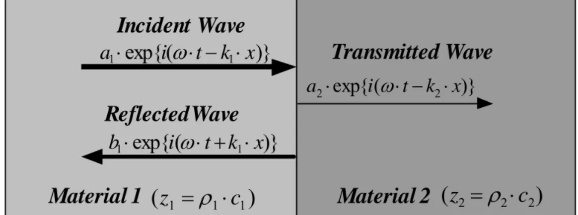
tried to evaluate the TBR by comparing with the heat flux ratio between the reference system without an interface and the system with an interface. They designated the system made up all the same molecules of argon as a reference system, and the system with an interface as a simulation system. Hereinafter, we will indicate the reference system as attached with the subscript of REF while the simulation system as attached with the subscript of SYS. They defined an energy reflection coefficient (ERC) from two heat fluxes, and then compared with the ERC evaluated from the AIMM. Assuming that an incident wave to an interface is a1exp
{
i(
ω⋅t −k1⋅x) }
, a reflected wave from it, and a transmitted wave through it (
{i t k x
b1exp ω⋅ + 1⋅ )} a2exp
{
i(
ω⋅t−k2⋅x) }
as shown in Fig.3, then the ERC is given as follows [21-23].2
1 2 1 2 2
1 1
2 2
1 1
2 2
1 1 1
1 ) (
⎟⎟
⎟⎟
⎟
⎠
⎞
⎜⎜
⎜⎜
⎜
⎝
⎛
+
−
=
⎟⎟
⎟⎟
⎠
⎞
⎜⎜
⎜⎜
⎝
⎛ +
−
=
m m m m
c c c c m
ERC
ρ ρρ ρ
(8)
Eq.(8) can be easily obtained because the acoustic velocity of a solid is given as the square root of the Young’s modulus divided by a density (c= Y/ρ ) and the intermolecular potentials of the two materials were assumed to be identical. Matsumoto et al. suggested that the ERC of Eq.(8) would be equal to the ERC of Eq.(9) if the same simulation conditions were applied to the system with an interface and the reference system without an interface.
SYS REF
REF SYS
R R q
q q
ERC = − • = −
• •
1 1
)
( (9)
Although the concept proposed by Matsumoto et al. was very simple to understand, easy to handle and showed some improved results compared with the AMM and the DMM, the deviation between Eq.(8) and Eq.(9) was still large.
Soon after the report of Matsumoto et al. [20], Choi et al. clarified that the failure of Matsumoto et al. resulted from the BCs of the AIMM [25]. Originally, the AIMM is used for the analysis of a wave reflection and transmission occurring at an interface of a macrosystem such as a string, a slender bar or a slinky [21-23]. Therefore, the BCs of the AIMM should be modified for a microscale system. Choi et al. suggested a new model, so called C-M model, to be used for the TBR evaluation of a microscale system.
Their model was also based on the AIMM but they modified the BCs to be suitable for a microscale system as briefly mentioned in the section 1. The predictions by the C-M model showed a good agreement with the heat flowrate ratios evaluated from the MD simulations; however, it was not the completed model because the influence due to a potential ratio was not included in it. The details of the C-M model and the updated one are given in the next two sections.
3-3. The previous C-M model
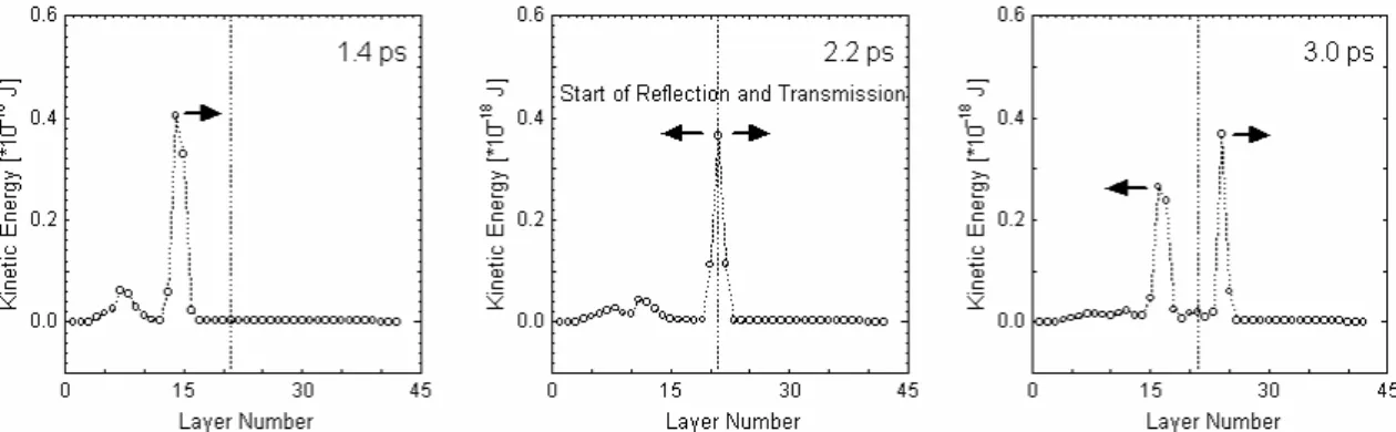
For the development of a new model based on the AIMM, Choi et al. investigated whether a wave reflection and transmission is still applicable to an ideal epitaxial interface from the viewpoint of a molecular size [25]. They applied a very weak pulse, which corresponded to the thermal motions of molecules, to one end of a system and confirmed that the applied pulse was partly reflected at an interface and the rest was transmitted over it as shown in Fig.4. After confirming that the classical wave theory for a macrosystem could be applied to a microscale system, they modified the BCs of the AIMM.
The BCs of the AIMM are (1) the displacements of both sides at an interface are the same for all time, and (2) the forces acting to both sides at an interface are also the same.
These conditions assure that there is no discontinuity of the displacement and the force at an interface. However, it is questionable whether the BC (1) is applicable to a
microscale system although the BC (2) can be considered to remain reasonable. Choi et al. assumed that the displacements of the molecules are not collective but rather random from a microscopic viewpoint. In a macroscale, the energy as the form of a wave is extremely large compared with the thermal energy due to molecular motion; therefore, the ERC can be sufficiently calculated by considering only the collective motion of a body. However, in the evaluation of the TBR at a solid interface, the energy level of a lattice vibration should be considered.
Suppose two molecules with the different masses but with the same L-J potential and their movements. Then, it can be easily imagined that the amplitudes of two molecules are different from each other and expected to be proportional to their mass ratio from the mechanical background. This situation results in that the BC (1) of the AIMM should be altered as (1’) the displacement ratio between two molecules at an interface is proportional to their mass ratio. However, the BC (2) is still applicable since an intermolecular force is the same under Newton’s third law, action and reaction law.
These modified BCs, (1’) and (2), are summarized as Eq. (10) and Eq. (11) from the classical wave theory [3,21-23].
2 2 1 1
1 a
m b m
a + = (10)
2 2 1 1 1
1 a Z b Z a
Z ⋅ + ⋅ =− ⋅
− (11)
In the above equations, a1 is the amplitude of an incident wave, b1 the one of a reflected wave, and a2 the one of a transmitted wave as shown in Fig.3. Z is an acoustic impedance of material, which is defined as a density times an acoustic velocity of a material. From the above-modified BCs, the ERC occurring at an interface can be theoretically derived as follows [25].
2
5 . 1
1 2
5 . 1
1 2
1 1 ) (
⎪⎪
⎭
⎪⎪
⎬
⎫
⎪⎪
⎩
⎪⎪
⎨
⎧
⎟⎟⎠
⎜⎜ ⎞
⎝ +⎛
⎟⎟⎠
⎜⎜ ⎞
⎝
−⎛
=
m m m m m
ERC (12)
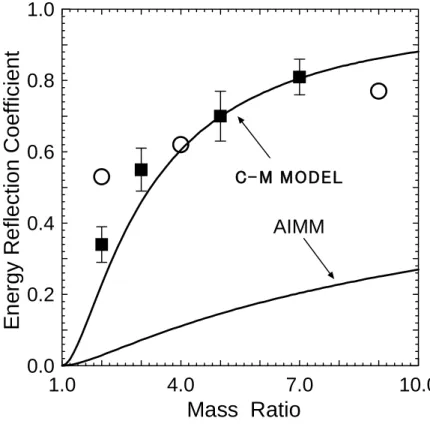
Eq.(12) is the result of the C-M model developed in our previous study, which reported that the heat flowrate ratio from the MD results showed the agreement within the maximum deviation of 20 % error when compared with the ERC by Eq. (12). Fig.5 shows the ERC by Eq.(8) of the AIMM, the ERC by Eq. (12) of the C-M model based on the modified BCs, (1’) and (2). For the comparison, the heat flowrate ratios from the MD simulations by Matsumoto et al. [20] and by Choi et al. [25] are shown together in it. As seen in the figure, the C-M model predicts accurately the ERC.
3-4. The updated C-M model
The purpose of this study is to complete the C-M model by including the effect by a potential ratio in the previous version. For this, the temperature jumps at an interface
were investigated by changing a molecular mass and a potential of the upper half of Fig.1. As shown in Fig.6 and 7, the heat flowrate decreased and a temperature jump became large as a mass ratio or a potential ratio increased. The temperature jump was observed more severe in the change of a mass ratio than in the change of a potential ratio. Fig.6 is the example of a heat flowrates and a temperature jump when the discontinuity of an interface was resulted from the difference in molecule’s mass; on the other hand, Fig.7 shows the same results when the interface was made by the difference in potentials. As already mentioned in the section 3.1, Fig.2 is the example that a mass ratio and a potential ratio were simultaneously changed. Comparing Fig.6 with Fig.7, we can clearly see that the TBR is more dependent on a mass ratio than a potential ratio since the TBR is directly related with a temperature jump or the reduction of a heat flowrate. Also, it seems that the TBR will increase when dissimilarity between two species gets to be large. However, if comparing Fig.2 with these figures, the degree of dissimilarity between two species is not always dominant because the temperature jump was decreased in Fig.2.
To incorporate the effect due to the potential ratio into the previous C-M model, the interaction between two species was presented as the mixing rule of Lotentz-Berthelot given by Eq.(13) [28,34] and we paid cautiously our attention to the relative movements of two molecules at both sides of an interface.
2 1
12 ε ε
ε = ⋅ (13)
For the simplicity of an analysis, only two molecules were considered, which were arranged with one-dimension as shown in Fig.8. If considering a sufficiently long period, the assumption with a fixed boundary is reasonable since the time averaged position of each molecule at both ends will be constant. Under the assumption that the intermolecular force is equal to each other, the molecule 1 feels the spring constant
2 1
1 2 ε ε
ε + ⋅ when it moves any distance and the molecule 2 feels ε2+2 ε1⋅ε2 . This means that the BC (1) of the AIMM should be modified as (1’’) the displacement ratio at both sides of an interface should be inversely proportional to the ratio of their respective equivalent spring constant; therefore, the BC (1) should be modified as Eq.(14). However, the BC (2) for the intermolecular force of Eq.(10) is still applicable without any modification because the we assumed that the intermolecular forces acting to two molecules are identical.
2 2 1 2
2 1 1
1
1 2
2 a
b
a ε ε ε
ε ε ε
⋅ +
⋅
= +
+ (14)
Based on the BCs of Eq.(11) and Eq.(14), the ERC can be derived as Eq.(15) if the interface results from dissimilarity due to the different potentials.
2
1 2
1 2 5 . 1
1 2
1 2
1 2 5 . 1
1 2
2 1
2 1
2 1
2 1
) (
⎥⎥
⎥⎥
⎥⎥
⎥⎥
⎥⎥
⎥⎥
⎦
⎤
⎢⎢
⎢⎢
⎢⎢
⎢⎢
⎢⎢
⎢⎢
⎣
⎡
⎪⎪
⎭
⎪⎪
⎬
⎫
⎪⎪
⎩
⎪⎪
⎨
⎧
+
⎟⎟ +
⎠
⎜⎜ ⎞
⎝
⎛ +
⎪⎪
⎭
⎪⎪
⎬
⎫
⎪⎪
⎩
⎪⎪
⎨
⎧
+
⎟⎟ +
⎠
⎜⎜ ⎞
⎝
⎛
−
=
ε ε
ε ε ε
ε
ε ε
ε ε ε
ε
ε
ERC (15)
Fig.9 shows the heat flowrate ratios obtained from the MD simulations and the ERCs predicted by the C-M model, which were calculated by Eq.(12) and Eq.(15). The simulations were performed separately in two cases, i.e. there exists only a mass ratio or only a potential ratio. It was confirmed that the predictions by the C-M model agreed well with the ERCs evaluated from the MD simulations. From Fig.9, it was observed that the ERC is more susceptible to the mass difference than the potential difference.
Finally, we tried to derive the equation for the ERC incorporating the effects of a potential ratio and a mass ratio. From the physical intuition, it can be easily imagined that there will be a superposition effect in the case that two species are simultaneously different from the masses and the potentials. This suggests that the ERC will be escalated by the contributions from two effects and leaded to the form of Eq.(16).
2
1 ) 1 ,
( ⎟⎟
⎠
⎜⎜ ⎞
⎝
⎛
⋅ +
⋅
= −
β α
β ε α
m
ERC (16)
5 . 1
1 2⎟⎟
⎠
⎜⎜ ⎞
⎝
=⎛ m
α m (17)
⎪⎪
⎭
⎪⎪
⎬
⎫
⎪⎪
⎩
⎪⎪
⎨
⎧
+
⎟⎟ +
⎠
⎜⎜ ⎞
⎝
⎛
=
1 2
1 2 5 . 1
1 2
2 1
2
ε ε
ε ε ε
ε
β (18)
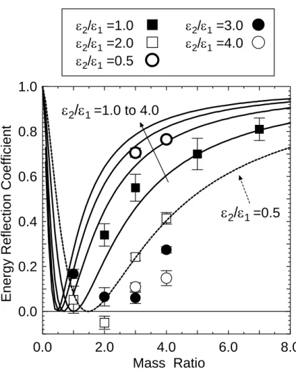
In Eq.(16), α presents the contribution by the mass ratio to the ERC and β is the same factor by the potential ratio. To confirm the correctness of Eq.(16), we simulated the various cases with changing the mass ratio and the potential ratio simultaneously. In contrast to our naive anticipation that the ERC may be calculated by Eq.(16) if considering the overall effects, however, the ERCs from the MD simulations are largely deviated from the predictions as shown in Fig.10. This means that the developed C-M model is not generalized but can be applied to only single effect due to a mass ratio or a potential ratio. After careful investigation of Fig.10, we noted that the ERCs from the heat flowrate ratio when ε2/ε1 is 2.0 are nearly the same as the predictions by the C-M
model when ε2/ε1 is 0.5. This implies the possibility that the displacement ratio between two molecules at an interface, designated as 1 and 2 in Fig.8, are not increased by the superposition of two effects but rather decreased by the cancellation of them. For the investigation of such a characteristic, the simulation of two degrees of freedom as shown in Fig.8 was performed and the relative displacement ratios between two molecules were measured. The results showed that the displacement ratio, when the interface was made by only the mass difference, was larger than that when the interface was made by the simultaneous difference in mass and potential. This characteristic can be explained theoretically. In accordance with the vibration theory of two degrees of freedom [35], the displacement ratio is derived as Eq.(19) and Eq.(20).
⎥⎥
⎥
⎦
⎤
⎢⎢
⎢
⎣
⎡
⎪⎭ +
⎪⎬
⎫
⎪⎩
⎪⎨
⎧
⎟⎟
⎠
⎞
⎜⎜
⎝
⎛ +
⎟−
⎟
⎠
⎞
⎜⎜
⎝
⎛ +
⎪⎭−
⎪⎬
⎫
⎪⎩
⎪⎨
⎧
⎟⎟
⎠
⎞
⎜⎜
⎝
⎛ +
⎟+
⎟
⎠
⎞
⎜⎜
⎝
⎛ +
⋅ − +
=
1 2 2
1 2 2
1 1
2 1
2 2
1 1
2 2
1 2 2
1 1 1 1 1 4
2 1 1
m m m
m m
m x
x
H
ε ε ε
ε ε
ε ε
ε ε
ε ε
ω
(19)
⎥⎥
⎥
⎦
⎤
⎢⎢
⎢
⎣
⎡
⎪⎭ +
⎪⎬
⎫
⎪⎩
⎪⎨
⎧
⎟⎟
⎠
⎞
⎜⎜
⎝
⎛ +
⎟−
⎟
⎠
⎞
⎜⎜
⎝
⎛ +
⎪⎭+
⎪⎬
⎫
⎪⎩
⎪⎨
⎧
⎟⎟
⎠
⎞
⎜⎜
⎝
⎛ +
⎟+
⎟
⎠
⎞
⎜⎜
⎝
⎛ +
⋅ − +
=
1 2 2
1 2 2
1 1
2 1
2 2
1 1
2 2
1 2 2
1 1 1 1 1 4
2 1 1
m m m
m m
m x
x
L ε
ε ε
ε ε
ε ε
ε ε
ε ε
ω
(20) Eq.(19) is the displacement ratio for the high frequency, ωH, which is the frequency of an anti-phase mode; Eq.(20) is for the low frequency, ωL, which is the frequency of a synchro-mode. Considering that the high frequency component will be dominant to the energy transfer, the displacement ratio has to be determined from Eq.(19) under the various combinations of the mass ratio and the potential ratio. Fig.11 depicts the displacement ratios of two molecules arranged as Fig.8, which were calculated by Eq.
(19). Therefore, the discrepancy in Fig.10 is resulted from the fact that the ERC is not escalated by the superposition of two effects due to the mass ratio and the potential ratio, but relaxed by the cancellation effect of them. Consequently, the coefficients of α and β in Eq.(16) should not be multiplied but divided as follows.
2
1 1 ) , (
⎟⎟
⎟⎟
⎠
⎞
⎜⎜
⎜⎜
⎝
⎛ +
−
= β αβ α ε
m
ERC (21)
In Fig.12, the ERCs from the MD simulations and the predictions given by Eq. (21) are shown together with. From the fact that Eq.(21) predicts accurately the ERCs from the MD simulations, it can be concluded that the developed C-M model is quite excellent compared with any other existing model such as the AMM, the DMM and the AIMM.
4. Conclusions
For the analysis of the TBR at an interface such as superlattices, the NEMD simulations were performed and the mechanism of the TBR could be explained through the wave reflection at an interface even though the related energy, which is due to the thermal motions of molecules, is very small. As described in the section 1, we had already the new model for the prediction of the TBR at an interface in thin films or superlattices. For the application of the conventional AIMM to a microscale system, the BCs of the AIMM were modified and the new concept was introduced, which is the heat flux ratio or the heat flowrate ratio between the simulation system and the reference system. However, it had the limited applicability since it took account of only the effect due to a mass ratio.
In this study, we completed the C-M model by including even the effect due to a potential ratio and confirmed that the predictions from our model agree well with the results from the MD simulations. The maximum deviation between the C-M model and the MD results was within 20 %. This is quite satisfactory result for an engineering usage. However, it must be noted that the applicability of the C-M model, which is purely based on a theoretical derivation, is limited on a non-conductor or a semiconductor that can be ignored the role of free electrons in the energy transfer.
Nevertheless, we are certain that the C-M model provides engineers with a simple tool to evaluate the TBR in thin films or superlattices. Furthermore, Eq.(21) proposes the ideal condition that the TBR does not occur at an interface since the ERC will be zero if α is equal to β in the numerator as follows.
5 . 1
1
1 2
1 2 5 . 1
1 2
1 2
2 1
2
⎪⎪
⎭
⎪⎪
⎬
⎫
⎪⎪
⎩
⎪⎪
⎨
⎧
+
⎟⎟ +
⎠
⎜⎜ ⎞
⎝
⎛
⎟⎟=
⎠
⎜⎜ ⎞
⎝
⎛
ε ε
ε ε ε
ε
m
m (22)
For the confirmation of the above condition, we simulated some preliminary simulations through the same method depicted in Fig.2 and observed that there existed really no wave reflection although we are still trying to obtain the complete results for it.
Aside from the feasibility that there exists the real materials to satisfy Eq.(22), it should be paid attention in that Eq.(22) provides engineers with the criterion on the ERC or the TBR of L-J potential materials at least. However, this study is not perfect because the mass ratios and the potential ratios were selected as fairly rough. Hence, there is a need to be continued some additional MD simulations with the smaller ratios in the masses and the potentials for raising the reliability of the C-M model.
References
[1] T. Shinjo, T. Takada, Metallic Superlattices-Artificially Structured Materials, Elsevier, Amsterdam, 1987.
[2] S. E. Lyshevski, Nano- and Microelectromechanical Systems, CRC press, New York, 2001.
[3] S. H. Choi, A Study on Thermal Conductivity of Thin Film by Molecular Dynamics Method, Ph. D. Dissertation, The University of Tokyo, 2003.
[4] M. I. Flik, B. I. Choi, K. E. Goodson, Heat Transfer Regimes in Microstructures, ASME J. of Heat Transfer 114 (1992) 666-674.
[5] S. Kotake, S. Wakuri, Molecular Dynamics Study of Heat Conduction in Solis Materials, JSME Int. J (B) 37 (1) (1994) 103-108.
[6] P. E. Phelan, Application of Diffuse Mismatch Theory to the Prediction of Thermal Boundary Resistance in Thin-Film High-Tc Superconductor, ASME J. Heat Transfer 120 (1998) 37-43.
[7] G. Chen, Particularities of Heat Conduction in Nanostructures, J. Nanoparticle Research 2 (2000) 199-204.
[8] D. G. Cahill, W. K. Ford, K. E. Goodson, G. D. Mahan, A. Majundar, H. J. Maris, R.
Merlin, S. R. Phillpot, Nanoscale Heat Transfer, J. Appl. Phy. 93 (2) (2003) 793-818.
[9] P. K. Shelling, S. R. Phillpot, P. Keblinski, Comparison of Atomic-Level Simulation Methods for Computing Thermal Conductivity, Phys. Rev. B 65 (2002) 144306/1-144306/12.
[10] G. Chen, Size and Interface Effects on Thermal Conductivity of Superlattices and Periodic Thin-Film Structures, ASME J. Heat Transfer 119 (1997) 220-229.
[11] G. Chen, Thermal conductivity and ballistic-phonon transport in the cross-plane direction of superlattices, Phys. Rev. B 57 (1998) 14958-14973.
[12] F. C. Chou, J. R. Lukes, X. G. Liang, K. Takahashi, C. L. Tien, Molecular Dynamics in Microscale Thermophysical Engineering, Ann. Rev. Heat Transfer 10 (1999) 141-176.
[13] J. R. Lukes, D. Y. Li, X. G. Liang, C. L. Tien, Molecular Dynamics Study of Solid Thin-Film Thermal Conductivity, ASME J. Heat Transfer 122 (2000) 536-543.
[14] S. G. Volz, G. Chen, Molecular-dynamics simulation of thermal conductivity of silicon crystals, Phys. Rev. B 61 (2000) 2651-2656.
[15] S. H. Choi, S. Maruyama, Calculation of Heat Conduction of Solid by Classical Molecular Dynamics Method, Proc. of 39th National Heat Transfer Symp. of Japan (2002).
[16] S. H. Choi, S. Maruyama, K. K. Kim, J. H. Lee, Evaluation of the Phonon Mean Free Path in Thin Films by Using Classical Molecular Dynamics, J. Kor. Phys. Soc. 43 (5) (2003) 747-753.
[17] M. E. Lumpkin, W. M. Saslow, One-Dimensional Kapitza Conductance- Comparison of the Phonon Mismatch Theory with Computer Experiments, Phys. Rev.
B 17 (1978) 4295-4302.
[18] W. A. Little, The Transfer of Heat between Dissimilar Solids at Low Temperature, Canadian J. Phys. 37 (1959) 334-349.
[19] E. T. Swartz, R. O. Pohl, Thermal Boundary Resistance, Rev. Mod. Phys. 61 (1989) 605-668.
[20] M. Matumoto, H. Yakayabashi, T. Makino, Thermal Resistance of Crystal Interface: Molecular Dynamics Simulation, J. of JSME (B) 68 (671) (2002) 87-93.
[21] H. J. Pain, The Physics of Vibration and Waves, John Wiley & Sons, New York,
1983.
[22] F. S. Crawford Jr., Waves, McGraw-Hill Publishing Company, New Yorks, 1994.
[23] J. Billingham, A. C. King, Wave Motion, Cambridge University Press, London, 2000.
[24] S. H. Choi, S. Maruyama, Thermal Boundary Resistance at Solid Interface by Molecular Dynamics Method, Proc. of 40th National Heat Transfer Symp. of Japan (2003).
[25] S. H. Choi, S. Maruyama, K. K. Kim, J. H. Lee, Feasibility Study of a New Model for the Thermal Boundary Resistance at Thin Film Interface, J. Kor. Phys. Soc. 44 (2) (2004) 317-325.
[26] R. J. Sadus, Molecular Simulation of Fluids-Theory, Algorithms, and Object - Orientation, Elsevier, Amsterdam, 1999.
[27] D. Frenkel, B. Smit, Understanding Molecular Dynamics - from Algorithms to Applications, Academic Press, New York, 1996.
[28] M. P. Allen, D. J. Tildesley, Computer Simulation of Liquids, Oxford Univ. Press, London, 1993.
[29] M. Haile, Molecular Dynamics Simulation-Elementary Methods, Wiley, New York, 1997.
[30] S. H. Choi, S. Maruyama, Variations in the Thermal Conductivity of Insulating Thin Films with Temperature and Pressure, J. Kor. Phys. Soc. 45 (4) (2004) 897-906.
[31] A. R. Abramson, C. L. Tien, A. Majumdar, Interface and Strain Effects on the Thermal Conductivity of Hetrostructures: A Molecular Dynamics Study, ASME J. Heat Transfer 124 (2002) 963-970.
[32] G. Chen and M. Neagu, Thermal Conductivity and Heat Transfer in Superlattices, Appl. Phys. Lett. 71 (19) (1997) 2761-2763.
[33] D. G. Cahill, A. Bullen, S. M. Lee, Interface Thermal Conductance and the Thermal Conductivity of Multilayer Thin Films, High Temperatures-High Pressures 32 (2000) 134-142.
[34] J. O. Hirschfelder, C. R. Curtiss, R. B. Bird, Molecular Thory of Gases and Liquids, Wiley, New York, 1964.
[35] L. Meirovitch, Fundamentals of Vibrations, McGraw-Hill, New Yorks, 2001.
Fig. 1. The simulation system of fcc<111>. [A] is a fixed adiabatic wall; [H] is the hot temperature control layers (TCLs); [C] is the cold TCLs. The total layer is 30 and a temperature gradient is measured in the medium of 18 layers excluding the TCLs and the fixed layers at both ends.
0 100 200 300 400 500 -10.0
-5.0 0.0 5.0 10.0
Time [pico sec]
Energy [10-18 J]
34 37 40 43 46 dqin/dt=1.4041X10-8 J/sec
qin+qout
dqout/dt=1.3968X10-8 J/sec
0 10 20 30 40 50 60 70 80 90
Temperature [K]
Z Directional Length [A] dT/dZ=-5.4162X108 K/m
P.E=3.0 Mass=4.0
o
(a) Heat flux (b) Temperature profile
dT/dZ=-1.2521X109 K/m
P.E=1.0 Mass=1.0
Fig. 2. The heat flowrates and the temperature profile of the system with the interface resulted from a potential ratio and a mass ratio. Half of the system is argon and the rest half consists of the molecules with four times mass and three times potential compared with argon. The dotted lines indicated by an arrow on (a) are the heat flowrates of the reference system.
Incident Wave
Reflected Wave
Material 1
Transmitted Wave
Material 2 )}
(
exp{
11
i t k x
a ⋅ ω ⋅ − ⋅
)}
(
exp{ 2
2 i t k x
a ⋅
ω
⋅ − ⋅)}
(
exp{
11
i t k x
b ⋅ ω ⋅ + ⋅
)
( z
1= ρ
1⋅ c
1( z
2= ρ
2⋅ c
2)
Fig. 3. A wave behavior at an interface in accordance with a classical wave theory. The part of an incident wave is partly transmitted through the interface and the rest is reflected. Z is an acoustic impedance, which is the inherent property of a material defined as a density times an acoustic velocity.
Fig. 4. Pulse reflection at an interface and transmission over it in the case that the mass ratio is 1 : 5. This figure was cited from the reference [25].
1.0 4.0 7.0 10.0 0.0
0.2 0.4 0.6 0.8 1.0
E n e rgy R e flection Coefficient
Mass Ratio
C? MODELAIMM C- M MODEL
Fig. 5. The ERC by the MD results and the models. Matsumoto et al. simulated with the system of fcc<100> (marked as ○) and compared the heat flux ratio obtained from the simulations with the prediction by the AIMM, however Choi et al.’s was on fcc<111>
(marked as ■) and compared the heat flux ratio with the prediction by the C-M model.
The C-M model displayed 20 % deviation at most, which shows an excellent agreement compared with any other existing model. The data were cited from the reference [20]
and [25].
0 100 200 300 400 -4.0
-2.0 0.0 2.0 4.0
Time [pico sec]
Energy [10-18 J]
37 38 39 40 41 42 43
dqin/dt=4.2036X10-9 J/sec Ein+Eout
dqout/dt=4.0812X10-9 J/sec
0 10 20 30 40 50 60 70 80 90
Temperature [K]
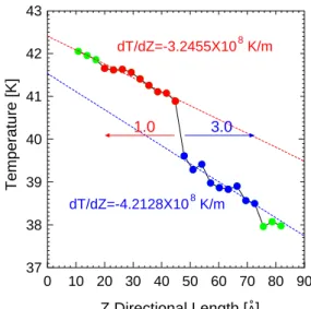
dT/dZ=-4.2128X108 K/m 3.0
(a) Heat flux (mass ratio; 1:3) (b) Temperature profile (mass ratio; 1:3) dT/dZ=-3.2455X108 K/m
1.0
0 100 200 300 400
-4.0 -2.0 0.0 2.0 4.0
Time [pico sec]
Energy [10-18 J]
dqout/dt=2.6473X10-9 J/sec dqin/dt=2.9300X10-9 J/sec
0 10 20 30 40 50 60 70 80 90 37
38 39 40 41 42 43
Temperature [K]
dT/dZ=-3.8642X108 K/m 5.0
(c) Heat flux (mass ratio; 1:5) (d) Temperature profile (mass ratio; 1:5) Z Directional Length [Ao]
Z Directional Length [Ao] dT/dZ=-1.8194X108 K/m
1.0
Fig. 6. The heat flowrates and the temperature profile of the system with the interface resulted from a mass ratio. (a) and (b) are the case that a mass ratio is 1:3, (c) and (d) are 1:5. A temperature jump is getting large as a mass ratio increased. The dotted lines indicated by the arrow are the same meaning as in Fig.2.
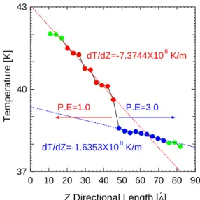
0 100 200 300 400 -6.0
-3.0 0.0 3.0 6.0
Time [pico sec]
Energy [10-18 J]
37 40 43 dqin/dt=8.2380X10-9 J/sec
Ein+Eout
dEout/dt=8.0470X10-9 J/sec
0 10 20 30 40 50 60 70 80 90
Temperature [K]
dT/dZ=-1.6353X108 K/m P.E=3.0 dT/dZ=-7.3744X108 K/m
P.E=1.0
0 100 200 300 400
-6.0 -3.0 0.0 3.0 6.0
Time [pico sec]
Energy [10-18 J]
Ein+Eout
dEout/dt=5.7550X10-9 J/sec dqin/dt=5.6613X10-9 J/sec
0 10 20 30 40 50 60 70 80 90 37
38 39 40 41 42 43
Temperature [K]
dT/dZ=-8.9878X107 K/m P.E=5.0
(a) Heat flux (potential ratio; 1:3) (b) Temperature profile (potential ratio; 1:3)
(c) Heat flux (potential ratio; 1:5) (d) Temperature profile (potential ratio; 1:5) Z Directional Length [Ao]
Z Directional Length [Ao] dT/dZ=-7.0285X108 K/m
P.E=1.0
Fig. 7. The heat flowrates and the temperature profile of the system with the interface resulted from a potential ratio. (a) and (b) are the case that the potential ratio is 1:3, (c) and (d) are 1:5. A temperature jump is getting large as the potential ratio increased.
From the comparison with Fig. 5, the TBR is more dependent on the mass ratio than the potential ratio. The dotted lines indicated by the arrow are the same meaning as in Fig.2.
Fig. 8. The simplified model for analyzing the displacement ratio of two molecules. The molecule 1 feels the spring constant ε1+2 ε1⋅ε2 when it moves any distance and the molecule 2 feels ε2+2 ε1⋅ε2 under the assumption that an intermolecular force is equal to each other.
0.0 2.0 4.0 6.0 8.0
0.0 0.2 0.4 0.6 0.8
1.00.0 2.0 4.0 6.0 8.0
Energy Reflection Coefficient
Mass Ratio Potential Constant
AIMM Potential Ratio
Mass Constant
Fig. 9. The ERC by the C-M model and the ERC by the MD simulations. The prediction of the C-M model is excellent and the maximum deviation is about 20 %. Solid squares present the heat flowrate ratios when the mass ratio was changed under the constant pontential; open squares the same ones when the potential ratio was changed under the constant mass; the dotted line is the prediction from the conventional AIMM. It can be seen that the ERC is more dependent on the mass difference than the potential difference.
0.0 2.0 4.0 6.0 8.0 0.0
0.2 0.4 0.6 0.8 1.0
Energy Reflection Coefficient
Mass Ratio
ε
2/ε
1=1.0 to 4.0ε
2/ε
1=0.5 ε2/ε1 =1.0ε2/ε1 =2.0
ε2/ε1 =3.0 ε2/ε1 =4.0 ε2/ε1 =0.5
Fig. 10. The ERC by the C-M model and the ERC by the MD simulations under the various combinations of the mass ratio and the potential ratio. The ERCs from the heat flowrate ratio when ε2/ε1 is 2.0 (marked as □) agree well with the predictions by the C-M model when ε2/ε1 is 0.5 (the dotted line). This is the clue to complete the C-M model.
0 2 4 6 8 10 0.0
5.0 10.0 15.0 20.0
Mass Ratio
| Relative Displacement |
ε2/ε1=1.0 to 4.0ε2/ε1=0.5
Fig. 11. The displacement ratio in the various combinations of the mass ratio and the potential ratio. These ratios are calculated through Eq.(18), which is the high frequency component. The displacement ratio with the mass ratio is larger than that with both of the mass ratio and the potential ratio. This means that the displacement ratio is not increased by the superposition of two factors but rather decreased by the cancellation effect of them.
0.0 2.0 4.0 6.0 8.0 0.0
0.2 0.4 0.6 0.8 1.0
Energy Reflection Coefficient
Mass Ratio
ε
2/ε
1=1.0 to 4.0ε
2/ε
1=0.5ε2/ε1 =1.0 ε2/ε1 =2.0
ε2/ε1 =3.0 ε2/ε1 =4.0 ε2/ε1 =0.5
Fig. 12. Comparison of the ERCs from the C-M model and the MD results. The lines are the predictions by the developed C-M model; the marks are the heat flowrate ratios obtained from the MD simulations in the various combinations of the mass ratios and the potential ratios. The ERCs from the MD simulations agree well with the predictions of the C-M model given by Eq. (20) within the maximum deviation of about 20 %.
![Fig. 1. The simulation system of fcc<111>. [A] is a fixed adiabatic wall; [H] is the hot temperature control layers (TCLs); [C] is the cold TCLs](https://thumb-ap.123doks.com/thumbv2/123deta/12310726.0/17.892.260.637.170.490/simulation-fixed-adiabatic-temperature-control-layers-tcls-tcls.webp)