PDF Asymptotic Properties of Branching Symmetric Markov Processes - Osaka U

(1)

Asymptotic Properties of Branching Symmetric Markov Processes

Yuichi SHIOZAWA

(2)

Acknowledgments

First and foremost, I would like to express my sincere gratitude to Professor Masayoshi Takeda for his pertinent guidance, insightful advice and warm encouragement throughout my master and doctoral programs. Without them, this thesis would never have been completed.

I am profoundly grateful to Professor Shinzo Watanabe for his invaluable suggestion. He led my interest to branching processes. I would like to thank Professor Zhen-Qing Chen for his helpful discussion and warm hospitality during my stay at University of Washington.

I am deeply thankful to Professor Tetsuya Hattori for his careful reading of the draft of this thesis and valuable advice. I wish to express my appreciation to Professors Takashi Kumagai and Toshihiro Uemura for their valuable comment and constant encouragement. I am grateful to Professor Yuu Hariya for his encouragement throughout the preparation of this thesis. My appreciation goes to Doctor Hiroshi Kawabi for his useful advice and great stimulus. I express my hearty thanks to Doctor Kaneharu Tsuchida for his sharing joys and sorrows with me throughout our master and doctoral programs. Finally, I would like to thank all the members of Tohoku Probability Seminar.

(3)

Introduction

It is well known that long time behaviors of Markov processes may follow rules such as central limit theorems, laws of large numbers, and large deviation principles. Some rules are controlled by principal eigenvalues. For example, M. Kac [37] proved that for a transient Brownian motion on R^d, the tail probability of the total occupation time on a compact set decays exponentially and its rate is given by the principal eigenvalue of the generator of a time changed Brownian motion. He also proved that the decay rate of a Feynman-Kac semigroup is given by the principal eigenvalue of the associated Schr¨odinger operator. Nowadays, this fact follows as a corollary of the Donsker-Varadhan large deviation theory ([23]). In this thesis, we study long time asymptotic properties of branching symmetric Markov processes in terms of the principal eigenvalues and the ground states of the associated Schr¨odinger type operators. In particular, we consider the extinction property, the growth rate of the numbers of particles, and the asymptotic distributions of particles.

A branching symmetric Markov process is known as a simple model of an evolving population.

Roughly speaking, a branching symmetric Markov process is described as follows: each particle moves on a state space according to the law of a symmetric Markov process until the splitting time, and then it creates new particles. After that, each of these particles repeats this movement independently. More precisely, let X be a locally compact separable metric space and m a positive Radon measure onX with full support. Let M= (Xt, Px) be anm-symmetric Markov process on X and M = (Xt,Px) the branching symmetric Markov process such that each particle moves independently according to the law of M. We denote by µ the branching rate, that is, the positive continuous additive functional (PCAF) A^µ_t in the Revuz correspondence to µ determines the distribution of the splitting time of each particle. We assume that µ is a Green-tight measure (in notation, µ ∈ K_∞). For the deﬁnition of the Green-tightness, see Deﬁnition 1.1. We denote by{p_n(x)}n≥0 thebranching mechanism, that is, a particle splits into n particles with probability pn(x) at branching site x ∈ X. Further, let Q(x) =P_∞

n=1npn(x) be the expected number of particles which are born at branching site x ∈ X and deﬁne the intensity of population growthby ν(dx) := (Q(x)−1)µ(dx).

We ﬁrst establish a criterion for M to extinct or extinct locally in terms of the principal eigenvalue for a time changed process. We deﬁne a formal operator by

Lˇ^µ,Qµ := 1

Qµ(L −µ), (1)

where L is the generator of M. We then see that ˇL^µ,Qµ is regarded as the generator of the exp (−A^µ_t)-subprocess time changed with respect toA^Qµ_t , whereA^Qµ_t is the PCAF corresponding to the measureQµ. SinceQµandµdenote the intensity of creations and the intensity of killings respectively, we say that the operator ˇL^µ,Qµexpresses the balance between these intensities. This suggests that the extinction of the branching process is controlled by the principal eigenvalue

(5)

of ˇL^µ,Qµ. In fact, the operator ˇL^µ,Qµ is realized as a self-adjoint operator on L²(X;Qµ) and λˇ:= ˇλ(Qµ, µ) denotes the bottom of the spectrum of ˇL^µ,Qµ, namely,

λ(Qµ, µ) = infˇ

½

E(u, u) + Z

X

u²dµ:u∈ F, Z

X

u²Qdµ= 1

¾

. (2)

Here (E,F) is the Dirichlet form generated by M. We then show that, under the assumption that ˇλis a discrete spectrum, the branching process M extincts or extincts locally if and only if ˇλ≥1 (see Theorems 2.4 and 2.11 below).

The extinction problem is one of the basic problems of branching Markov processes and has been studied by many persons. For instance, Sevast’yanov [49] and S. Watanabe [61] con- sidered this problem for a branching Brownian motion on a bounded domain in R^d with state- independent branching rate and branching mechanism. They then gave a criterion for extinction by the principal eigenvalue of the Dirichlet Laplacian. R. G. Pinsky [42] investigated and devel- oped the theory of generalized principal eigenvalues of Schrödinger operators. Using this theory, he in [43] analytically gave a criterion for a measure-valued branching diffusion process to extinct locally, that is, the particles on every compact set disappear. On the other hand, Engländer and Kyprianou [26] probabilistically gave the criterion for local extinction. In these papers, the ground state of the Schrödinger operator plays an essential role; they construct the ground state by using well-known facts for elliptic differential operators, Harnack’s inequality and Schauder’s estimate. Here we consider the branching jump Markov processes and this approach is not applicable to construct the ground state because we do not know the corresponding properties for non-local operators. To overcome this difficulty, we use the generator of a time changed process.

We can then construct the ground state by using the compact embedding of the Dirichlet form corresponding to the motion component; however, we must restrict the branching rate within the class K∞ to show the compact embedding. Further, to prove the regularity of the ground state, we need to restrict the branching rate within the subclassS_∞⊂ K_∞, which is introduced in [14] (see Deﬁnition 1.1). This assumption on the branching rate essentially says that the branching is rare at inﬁnity. Here we would like to emphasize that our result is an extension of the result in [49] and [61] because every constant function belongs to S_∞for Brownian motions on bounded domains. Moreover, we allow the state spaces to be unbounded and the branching rate to be not only functions but also measures.

We next study the exponential growth of the numbers of particles for the branching process M. To cope with this problem, we use the principal eigenvalue and the ground state of an associated Schr¨odinger operator. More precisely, let

L^ν :=L+ν (3)

and denote byλ1:=λ1(ν) the bottom of the spectrum of L^ν: λ₁(ν) = inf

½

E(u, u)− Z

X

u²dν :u∈ F, Z

X

u²dm= 1

¾

. (4)

Let h be the corresponding ground state. Namely, h is a function onX attaining the inﬁmum of (4). Deﬁne

M_t=e^λ¹^t

Zt

X

i=1

h¡ Xⁱ_t¢

, t≥0,

where Z_t denotes the total number of particles and Xⁱ_t, 1 ≤ i≤ Z_t, is the position of the ith particle at time t. Then, under the assumption that λ1 is a negative discrete spectrum, we

(6)

prove the square integrability of the martingale M_t. As a result, a limit M_∞ := lim_t_→∞M_t exists in L¹(Px) and Px-a.s. Furthermore, we show that the limit M_∞ is positive Px-a.s. on the event that the branching process survives (Theorem 3.4). This result says that Z_t grows exponentially with rate −λ₁ at least. We also study the exponential growth of the number of particles in every relatively compact open set (Theorem 3.8). Theorem 3.8 indicates that the number of particles in every relatively compact open set may grow exponentially at rate −λ₁. Engl¨ander and Kyprianou [26] studied the same problem for a branching diﬀusion process with regular branching rate function. Here we consider more general branching symmetric Markov processes than those studied in [26]. Indeed, we discuss the exponential growth for the branching processes whose motion components are jump Markov processes and whose branching rates are measures.

As stated above, the square integrability of Mt is crucial. We now explain how to prove it.

By the deﬁnition of the branching symmetric Markov process, it follows that E_x£

M_t²¤

=e^2λ¹^tE_x£

exp (A^ν_t)h(X_t)²;t < ζ¤ +E_x

·Z _t_∧_ζ

0

exp (2λ₁s+A^ν_s)h(X_s)²dA^Rµ_s

¸

, (5)

where ζ is the lifetime of M, A^ν_t = A^Qµ_t −A^µ_t and R(x) = P_∞

n=0n(n−1)pn(x). Hence, to show the square integrability of M_t, we use a criterion for the gaugeability of measures. Here µ=µ⁺−µ⁻∈ K_∞− K_∞ is said to begaugeableif

sup

x∈X

E_x h

exp

³ A^µ_ζ

´i

<∞.

Z.-Q. Chen [14] and Takeda [52] then showed thatµis gaugeable if and only if ˇλ(µ⁺, µ⁻)>1 (see Theorem 1.2 below). In addition, there are relations betweenλ1(µ) and ˇλ(µ⁺, µ⁻) as follows:

λ₁(µ)≥0 ⇐⇒ λ(µˇ ⁺, µ⁻)≥1 and λ₁(µ)>0 =⇒λ(µˇ ⁺, µ⁻)>1.

Applying these results to the right hand side of (5), we establish the square integrability of Mt. We ﬁnally establish limit theorems for a class of branching symmetric Markov processes.

Namely, under the assumption that λ1 is a negative discrete spectrum, we show that for any x∈X,Px-a.s.

tlim→∞e^λ¹^tZt(A) =M_∞ Z

A

h dm (6)

for every relatively compact Borel set A inX, whereZ_t(A) denotes the number of particles on the set A at time t (Theorem 4.7). The equation (6) says that Z_t(A) grows exponentially at rate −λ1 and that the ground state determines the asymptotic distribution of particles. The limit theorem for branching symmetric Markov processes has been studied for a long time. For example, S. Watanabe studied in [61] and [62] the asymptotic properties of branching symmetric diﬀusion processes and established a limit theorem in [62]. His approach is based on a general- ization of the Fourier transform and requires that the transition densities of the Feynman-Kac semigroups are represented by the spectral measures and the eigenfunctions. Asmussen and Hering [4] also established a limit theorem in [4] for general supercritical branching processes.

To apply their result to branching symmetric Markov processes, we have to check that every spectrum of the Schr¨odinger operator is discrete, and consequently the Feynman-Kac semigroup has an eigenfunction expansion. However, branching symmetricα-stable processes with singular

(7)

branching rates do not satisfy the conditions imposed in [62] and [4]. In fact, since the transition density ofL^ν may not be expressed by the spectral measure, the methods used in S. Watanabe [62] and in Asmussen and Hering [4] are not applicable here. Unlike their conditions, we use the fact that the operator L^ν has a spectral gap. A crucial point is that the spectral gap implies the ergodicity of theh-transformed semigroup of the Feynman-Kac semigroup. By this property with an application of the gaugeability of measures, we can establish (6) in discrete time, and then extend it to a continuous time version by applying a method from the proof of Theorem 1’ in [4].

We consider branching Brownian motions and branching symmetric α-stable processes as concrete models; a Brownian motion is a typical model of diffusion processes and a symmetric α-stable process is a typical model of jump processes. As we saw above, we need to calculate explicitly the principal eigenvalues ˇλ and λ1 in order to find asymptotic properties for these processes. However, it is difficult in general to calculate the principal eigenvalues of Schrödinger type operators with non-local principal parts. Therefore, for special classes of them, we calculate the principal eigenvalues by the Dirichlet principle. We can then obtain asymptotic properties explicitly for a class of branching Brownian motions and branching symmetricα-stable processes.

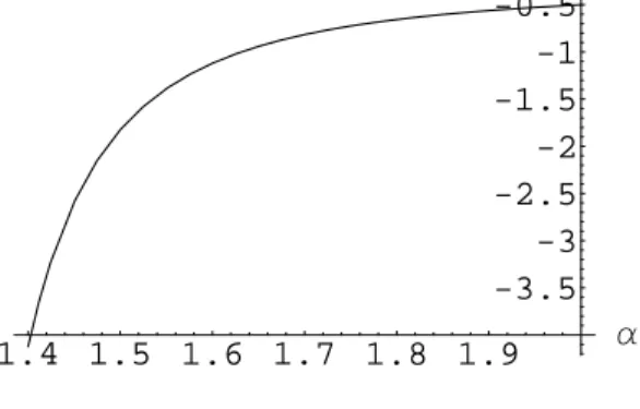
For example, let us consider a branching symmetric α-stable process in one dimension with 1 < α ≤ 2. First take the Dirac measure at a > 0 as branching rate and suppose that each particle dies upon arriving at 0. We then see that this branching symmetric α-stable process extincts if and only if

0< a≤



−Γ(α) cos

³πα 2

´

2





1/(α−1)

(Example 2.18). Next take δ0, the Dirac measure at the origin, as branching rate and suppose that the state space is R. We then obtain for anyx∈R,P_x-a.s.

tlim→∞e^λ¹^(α)tZ_t((−r, r)) =



 µZ _∞

−∞h dx−O¡ r⁻^α¢¶

M_∞, 1< α <2 2(1−e⁻^r)M_∞, α= 2 for anyr >0, where

λ₁(α) =−





2^1/α αsin

³π α

´





α/(α−1)

is the principal eigenvalue of the Schr¨odinger operator−¹₂(−∆)^α/2+δ₀andhis the corresponding ground state. Moreover,M_∞ is positiveP_x-a.s. (Example 4.12).

Since the explicit calculations of the principal eigenvalues are difficult as we mentioned above, we try to give lower bound estimates. To do this, we first establish a variational formula for Dirichlet forms. Recall that X be a locally compact separable metric space and m is a positive Radon measure onX with full support. In [24], Donsker and Varadhan proved a large deviation principle of occupation distributions of conservative Markov processes onX with the so-called I-function as its rate function. Moreover, they showed that, if the Markov process is m-symmetric, then the I-function is identified with the associated Dirichlet form (E,F). M.

F. Chen [13] then extended this identiﬁcation to symmetric jump processes with killings. Our objective is to extend it further to general symmetric Markov processes including time changed processes. More precisely, let ˆL be the “extended generator” of a symmetric Markov process

(8)

determined by the martingale problem and D⁺³ Lˆ´

the set of nonnegative functions in the domain of ˆL (see Deﬁnition 5.1). We then prove

E(f, f) =− inf

u∈D⁺(L^ˆ)^{, ε>0} Z

X

Lˆu

u+εf²dm, f ∈ F. (7)

Furthermore, applying this formula, we obtain the lower bound estimate of the bottom of the spectrum: let λ₀ be the bottom of the spectrum of the operator L. We can then derive the followinggeneralized Barta’s inequality,

λ0 ≥ inf

x∈X

Ã−Lˆu u

!

(x), u∈ D⁺⁺³ Lˆ´

,

whereD⁺⁺³ Lˆ´

is the set of strictly positive functions in the domain of ˆL (Theorem 5.8).

The organization of this thesis is as follows. In Chapter 1, we ﬁrst recall the notions of Dirichlet forms and symmetric Markov processes. We next introduce two classes K_∞ and S_∞ of Kato measures, which play an important role in this thesis. We next introduce the notion of branching symmetric Markov processes. We ﬁnally introduce the notion of symmetric α- stable processes because we consider branching symmetric α-stable processes as typical models.

Chapters 2, 3 and 4 are devoted to the study of asymptotic properties of branching symmetric Markov processes and its applications to branching Brownian motions and branching symmetric α-stable processes. We give in Chapter 2 a criterion for extinction or local extinction in terms of the principal eigenvalues for time changed processes. We study in Chapters 3 and 4 the exponential growth of the numbers of particles and the asymptotic distributions of particles in terms of the principal eigenvalues and the ground states of Schrödinger operators. Chapters 5 and 6 are devoted to calculations and estimates of the principal eigenvalues for Schrödinger type operators. We establish in Chapter 5 a variational formula for Dirichlet forms generated by general symmetric Markov processes. As its application, we derive generalized Barta’s inequality. Using this inequality and the Dirichlet principle, we estimate and calculate in Chapter 6 the principal eigenvalues of Schrödinger type operators associated with Brownian motions and symmetric α-stable processes. In Appendix A, we show that the Green function is positive for any absorbing symmetricα-stable process on an open set. This result implies that any absorbing α-stable process is irreducible even if the state space is disconnected.

Chapter 4 is based on a joint work with Zhen-Qing Chen and Chapter 5 is based on a joint work with Masayoshi Takeda.

(9)

Chapter 1

Preliminaries

In this chapter, we ﬁrst review the general theory of Dirichlet forms and some facts related to Feynman-Kac functionals. We next introduce the notion of branching Markov processes. We ﬁnally introduce the notion of symmetric α-stable processes and remark some properties.

1.1 Dirichlet forms and symmetric Hunt processes

LetX be a locally compact separable metric space andma positive Radon measure on Xwith full support. Let M = (Ω,F,Ft, θ_t, X_t, P_x, ζ) be an m-symmetric Hunt process on X, where {Ft}t≥0 is the minimal admissible ﬁltration. The shift operator θt satisﬁes Xt◦ θs = Xt+s

identically fors, t≥0, and ζ is the lifetime, ζ = inf{t >0 :Xt= ∆}, where ∆ is the cemetery point.

Let us denote by(E,F) the regular Dirichlet form ofM. LetFebe the family ofm-measurable functions on X such that |u| < ∞ m-a.e. and there exists an E-Cauchy sequence {un} of functions in F such that lim_n_→∞u_n = u m-a.e. Then (E,Fe) is called the extended Dirichlet form of (E,F) ([29, p. 36]). We deﬁne the 1-capacity associated with the Dirichlet form (E,F) for an open set O⊂X by

Cap₍₁₎(O) = inf{E1(u, u) :u∈ F, u≥1m-a.e. onO}, (1.1) whereEα(u, u) =E(u, u) +αR

Xu²dm forα >0, and for any set A⊂X by Cap₍₁₎(A) = inf

n

Cap₍₁₎(O) :O is open, O⊃A o

.

For a set A ⊂ X, a statement depending on x ∈ A is said to hold q.e. on A, if there exists a set N ⊂ A of zero capacity such that the statement is true for x ∈ A\N. Here q.e. is an abbreviation for quasi everywhere. A functionu ∈ Fe is said to be quasi continuous, if for any ε >0, there exists an open set O ⊂X with Cap₍₁₎(O)< εsuch thatu|X\O is ﬁnite continuous, whereu|X\O is the restriction ofu onX\O. It is then known in Theorem 2.1.7 of [29] that each u∈ Fe admits a quasi continuousm-version. In the sequel, we always assume that each u∈ Fe

is quasi continuous.

An increasing sequence{Fn}of closed sets is said to be a nestif limn→∞Cap₍₁₎(X\Fn) = 0.

An increasing sequence{F_n}of closed sets is said to be a generalized nestif lim_n_→∞Cap₍₁₎(K\ Fn) = 0 for any compact set K ⊂ X. A positive Borel measure µ is said to be smooth, if µ charges no set of zero capacity and there exists a generalized nest {Fn} such thatµ(Fn) <∞

(10)

for all n. Denote by S the set of smooth measures. It is then known in Theorem 5.1.4 of [29]

that there exists a one to one correspondence between smooth measures and positive continuous additive functionals (PCAFs in abbreviation), the so-calledRevuz correspondence, as follows; if we denote byA^µ_t the PCAF corresponding to µ∈ S, then for anyγ-excessive functionh(γ≥0) and any positive Borel measurable functionf,

limt↓0

1 t

Z

X

E_x

·Z _t

0

f(X_s)dA^µ_s

¸

h(x)m(dx) = Z

X

f(x)h(x)µ(dx).

A positive Radon measureµ on X is said to be ofﬁnite energy integral, if Z

X

|u|dµ≤Cp

E1(u, u), u∈ F ∩C₀(X) (1.2)

for some positive constantC, whereC0(X) stands for the set of continuous functions onXwith compact support. Denote byS0 the set of measures of ﬁnite energy integral. Then, by the Riesz representation theorem, there exists a unique functionG_αµ∈ F forµ∈ S0 such that

Eα(Gαµ, u) = Z

X

u dµ, u∈ F (1.3)

for anyα >0 ([29, Theorem 2.2.5]). We call G_αµtheα-potential ofµ.

For anyµ∈ S, there exists a generalized nest{Fn}such thatµn=1Fn·µ∈ S0([29, Theorem 2.2.4]). Then Lemma 2.2.10 of [29] implies thatG_αµ_n−G_αµ_m is again anα-potential forn > m, and consequently{G_αµ_n}is an increasing sequence. We thus deﬁne theα-potential ofµ∈ S by Gαµ= limn→∞Gαµn. We next characterize Gαµ probabilistically. LetA^µ_t be the PCAF whose Revuz measure isµ. Then

G_αµ_n(x) =E_x

·Z _ζ

0

e⁻^αtχ_F_n(X_t)dA^µ_t

¸

q.e. x∈X.

Since {Fn} is a generalized nest, it holds that

nlim→∞Ex

·Z ζ 0

e⁻^αtχFn(Xt)dA^µ_t

¸

=Ex

·Z ζ 0

e⁻^αtdA^µ_t

¸ . Hence we get

G_αµ(x) =E_x

·Z _ζ

0

e⁻^αtdA^µ_t

¸

q.e.x∈X. (1.4)

Denote by S1 the set of positive Radon measures on X charging no set of zero capacity. Then S0 ⊂ S1⊂ S.

When Mis transient, the 0-order capacity Cap(A) is defined by replacingE1 andF in (1.1) withE andFe, respectively. We say that a positive Radon measureµonXis said to beof finite (0-order) energy integral, if the inequality (1.2) holds with E1 on the right hand side replaced by E. Denote by S₀⁽⁰⁾ the set of measures of 0-order finite energy integral. Then the equation (1.3) with α = 0 determines a unique function Gµ ∈ Fe for any µ ∈ S₀⁽⁰⁾. We call Gµ the (0-order) potential of µ. By the same argument as above, we can defineGµ for any µ∈ S by Gµ= limn→∞Gµn, whereµn=1Fn·µandFn is a generalized nest such thatµn∈ S0. We also see that

Gµ(x) =E_x h

A^µ_ζ i

q.e. x∈X. (1.5)

(11)

Let (N, H) be a L´evy system of M (see [8] and [29, Theorem 5.3.1]); that is, N is a kernel on (X∆,B(X∆)) such thatN(x,{x}) = 0 for anyx∈X and Ht is a PCAF of Msuch that, for any nonnegative functionϕ∈ B(X_∆×X_∆) withϕ(x, x) = 0 for any x∈X_∆,

Ex



X

s≤t

ϕ(Xs−, Xs)



=Ex

·Z _t

0

Z

X_∆

ϕ(Xs, y)N(Xs, y)dHs

¸ ,

whereX_∆=X∪ {∆} andX_t₋ = lim_s_↑_tX_s. Denote byµ_H the Revuz measure of the PCAFH_t of Mand deﬁne

J(dx, dy) :=N(x, dy)µ_H(dx) and κ(dx) :=N(x,∆)µ_H(dx), (1.6) which are called the jump measure and the killing measure of M, respectively.

By Fukushima’s decomposition [29, Theorem 5.2.2], it holds that for u∈ Fe,

u(X_t)−u(X₀) =M_tû+N_tû, t≥0 P_x-a.s. for q.e. x∈X, (1.7) where M_tû is a martingale additive functional of finite energy andN_tû is a continuous additive functional of zero energy. Denote by M_tû,c and µ_⟨_Mû,c_⟩, respectively, the continuous martingale part of M_tû and the Revuz measure corresponding to ⟨Mû,c⟩_t, the quadratic variation of M_tû,c. The measureµ_⟨_Mû,c_⟩is called theenergy measureofM_tû,c. A Beurling-Deny decomposition ([29, Theorem 5.3.1]) then implies that

E(u, u) = 1 2

Z

X

µ_⟨_M^u,c_⟩(dx) + 1 2

ZZ

X×X\△(u(x)−u(y))²J(dx, dy) + Z

X

u(x)²κ(dx), u∈ F, where△={(x, y)∈X×X:x=y}.

Let M^µ = (X_t^µ, Px^µ), µ ∈ S1, be the subprocess of M with respect to the multiplicative functional exp (−A^µ_t) (see [29, Appendix A.2] for details):

E_x^µ[f(X_t^µ)] =Ex[exp(−A^µ_t)f(Xt);t < ζ].

Then M^µgenerates the regular Dirichlet form (E^µ,F^µ) ([29, Theorem 6.1.1]):

F^µ=F ∩L²(X;µ) E^µ(u, u) =E(u, u) +

Z

X

u²dµ, u∈ F^µ. Denote by τ_t^µ the right continuous inverse of A^µ_t,

τ_t^µ= inf n

s >0 :A^µ_s_∧_ζ > t o

.

LetF = supp[µ] and let F^µ be the ﬁne supportof the measure µdeﬁned by

F^µ={x∈X:P_x(τ₀^µ= 0) = 1}. (1.8) Note thatF^µ is ﬁnely closed and A^µ_t(ω) increases only when Xt(ω)∈F^µ forPx-a.s. ω∈Ω for q.e. x ∈ X ([29, Lemma 5.1.11]). The time changed process Mˇ = (Y_t^µ, P_x) of M with respect

(12)

toA^µ_t is deﬁned byY_t^µ=X_τ^µ

t. Then ˇMis aµ-symmetric Hunt process onF^µ with lifetime A^µ_ζ ([29, Theorem 6.2.1]). Set

HF^µu(x) =Ex[u(Xσ_{F µ});σF^µ <∞],

whereσF^µ is the hitting time ofF^µ,σF^µ = inf{t >0 :Xt∈F^µ}. Then ˇMgenerates the regular Dirichlet form ( ˇE,Fˇ) on L²(F;µ) ([29, Theorem 6.2.1]):

Fˇ=©

ψ∈L²(F;µ) :ψ=u µ-a.e. onF for someu∈ Fe

ª

Eˇ(ψ, ψ) =E(H_F^µu, H_F^µu), ψ∈Fˇ, ψ=u µ-a.e. onF for someu∈ Fe. Moreover, ( ˇE,Fˇ) satisﬁes

Eˇ(u, u) = inf{E(v, v) :v∈ Fe, v=u q.e. onF}. (1.9) The equation (1.9) is the so-called Dirichlet principle.

1.2 Gaugeability and Feynman-Kac semigroups

1.2.1 Gaugeability and classes of measures

Let{pt, t≥0} be the Markovian transition semigroup ofM given by ptf(x) =Ex[f(Xt)], f ∈ B⁺(X),

whereB⁺(X) denotes the set of nonnegative Borel measurable functions onX. In this subsection, we assume that the transition density ofMis absolutely continuous with respect tomand denote by p_t(x, y) the integral kernel ofp_t,

ptf(x) = Z

X

pt(x, y)f(y)m(dy).

LetG_α(x, y) be theα-resolvent density of M, G_α(x, y) =

Z _∞

0

e⁻^αtp_t(x, y)dt, α >0.

IfM is transient, then the Green function G₀(x, y) :=

Z _∞

0

p_t(x, y)dt exists forx̸=y, and we put G(x, y) =G0(x, y).

We now introduce classes of measures inS.

Deﬁnition 1.1. (i) A positive smooth Radon measure onX is said to be in the Kato classK, if

αlim→∞sup

x∈X

Z

X

G_α(x, y)µ(dy) = 0.

(ii) A positive smooth Radon measure on X is said to be in K_∞(G_α), if for any ε > 0, there exists a compact set K⊂X and a positive constant δ >0 such that

sup

x∈X

Z

X\K

G_α(x, y)µ(dy)< ε,

(13)

and for all measurable sets B ⊂K withµ(B)< δ, sup

x∈X

Z

B

Gα(x, y)µ(dy)< ε.

The class K_∞ is deﬁned by

K_∞=

(K∞(G), Mis transient K_∞(G₁), Mis recurrent.

(iii) A positive smooth Radon measure µonX is said to be in S∞(Gα), if for any ε >0, there exists a compact set K⊂X and a positive constant δ >0 such that

sup

(x,z)∈X×X\△

Z

X\K

Gα(x, y)Gα(y, z)

Gα(x, z) µ(dy)< ε, and for all measurable sets B ⊂K withµ(B)< δ,

sup

(x,z)∈X×X\△

Z

B

Gα(x, y)Gα(y, z)

Gα(x, z) µ(dy)< ε.

When M is transient, the class S_∞(G) is simply denoted by S_∞

If M is transient, then it holds that S_∞ ⊂ K_∞ by Corollary 3.1 of [19] and any measure in K_∞ with compact support belongs to S_∞. It is known in Proposition 2.2 of [14] that any measure µinK∞ isGreen bounded,

sup

x∈X

E_x h

A^µ_ζ i

= sup

x∈X

Z

X

G(x, y)µ(dy)<∞. (1.10) In the sequel, we assume that M is transient. Let µ be a signed measure onX which can be decomposed into µ = µ⁺−µ⁻ for some µ⁺, µ⁻ ∈ K_∞. Then the measure µ is said to be gaugeable, if

sup

x∈X

E_x h

exp

³ A^µ_ζ

´i

<∞, whereA^µ_t =A^µ_t⁺−A^µ_t⁻. Deﬁne

λ(µˇ ⁺, µ⁻) = inf

½

E(u, u) + Z

X

u²dµ⁻:u∈ F, Z

X

u²dµ⁺= 1

¾

. (1.11)

When µ⁻= 0, we simply denote ˇλ(µ⁺,0) by ˇλ(µ).

Theorem 1.2. ([14, Corollary 2.9, Theorem 5.1]) Suppose that a signed measure µ on X can be decomposed into µ = µ⁺−µ⁻ for some µ⁺, µ⁻ ∈ K∞. Then the following conditions are equivalent:

(i) The measure µ is gaugeable;

(ii) ˇλ(µ⁺, µ⁻)>1;

(iii) sup_x_∈_XE_xhR_ζ

0 exp (A^µ_t) dA^ν_t i

<∞ for any ν ∈ K_∞.

(14)

The implications (i) ⇔(ii) and (iii)⇒(ii) are already proved in [14, Corollary 2.9, Theorem 5.1]. We can show the implication (ii) ⇒ (iii) in a similar way to that yielding Proposition 3.2 of [15] as follows. Let µ be a measure on X which can be decomposed into µ = µ⁺−µ⁻ for someµ⁺, µ⁻∈ K_∞. Assume that ˇλ(µ⁺, µ⁻)>1 and ﬁx a measureν ∈ K_∞. Since

λ(pµˇ ⁺, pµ⁻)≥λ(pµˇ ⁺, µ⁻) = 1

pˇλ(µ⁺, µ⁻)

for any p > 1, we can take p > 1 such that ˇλ(pµ⁺, pµ⁻) > 1. Let q > 1 be the conjugate component ofp, that is,q satisﬁes 1/p+ 1/q = 1. Then the H¨older inequality implies that

Ex

·Z ζ 0

exp (A^µ_t) dA^ν_t

¸

≤Ex

"

sup

0≤t≤ζ

(exp (A^µ_t))A^ν_ζ

#

≤E_x

"

sup

0≤t≤ζ

(exp (A^pµ_t ))

#1/p

E_x h

A^qν_ζ i1/q

.

(1.12)

Noting that the measureqνbelongs toK_∞, we have sup_x_∈_XE_x h

A^qν_ζ i

<∞. A direct calculation yields that

sup

0≤t≤ζ

(exp (A^pµ_t )) = sup

0≤t≤ζ

Z _t

0

exp (A^pµ_s ) dA^pµ_s + 1

≤ sup

0≤t≤ζ

Z _t

0

exp (A^pµ_s )dA^p˜_s^µ⁺+ 1

= Z _ζ

0

exp (A^pµ_s )dA^p˜_s^µ⁺+ 1,

where ˜µ⁺−µ˜⁻ is the Jordan decomposition of the measure µ. Since the measures ˜µ⁺ and ˜µ⁻ belong to the class K_∞, respectively, and the condition that ˇλ(pµ⁺, pµ⁻) >1 is equivalent to that ˇλ(pµ˜⁺, pµ˜⁻)>1 by [58, Lemma 3.1], we obtain

x∈XsupE_x

·Z _ζ

0

exp (A^pµ_t )dA^p˜_t^µ⁺

¸

<∞

by [14, Corollary 2.9, Theorem 5.1]. Therefore, the right hand side of (1.12) is bounded, which shows the implication (ii) ⇒ (iii).

1.2.2 Feynman-Kac semigroups

In this subsection, we assume the following on M:

Assumption 1.3. (i) (Irreducibility) If a Borel setAispt-invariant, that is, ifpt(1Af) =1Aptf holds for everyf ∈L²(X;m)∩ Bb(X) andt >0, then either m(A) = 0 or m(X\A) = 0 holds.

Here Bb(X) stands for the set of bounded Borel measurable functions onM.

(ii) (Strong Feller property) For any f ∈ Bb(X), ptf is a bounded and continuous function on X.

(iii) (Ultracontractivity) For any t > 0, it holds that ∥pt∥1,∞ < ∞, where ∥ · ∥p,q denotes the operator norm fromL^p(X;m) toL^q(X;m).

(15)

Note that, by Assumption 1.3 (ii) and the m-symmetry of p_t, the transition probability of Mis absolutely continuous with respect to m.

We know from [50] that, for a positive smooth measure µof Mon X and α >0, Z

X

u²dµ≤ ∥Gαµ∥∞Eα(u, u), u∈ F.

Then, by the deﬁnition of K, it follows that for µ∈ K, there exists a constant α >0 such that Z

X

u²dµ≤ 1

2E(u, u) +α Z

X

u²dm foru∈ F. (1.13)

Let µ be a signed measure on E which can be decomposed as µ = µ⁺ −µ⁻ for some µ⁺, µ⁻∈ K. Let{p^µ_t, t≥0} be the Feynman-Kac semigroup given by

p^µ_tf(x) =E_x[exp (A^µ_t)f(X_t)], f ∈ B⁺(X). (1.14) Then it follows from [1, Theorem 3.3] and (1.13) above that{p^µ_t, t≥0}is a strongly continuous semigroup onL²(X;m) and its associated quadratic form is (E^µ,F) where

E^µ(u, u) =E(u, u)− Z

X

u²dµ, u∈ F. Moreover, under Assumption 1.3, we have from [1] the following.

Theorem 1.4. Let µ=µ⁺−µ⁻∈ K − K. Then, under Assumption 1.3, it holds that

(i) For any f ∈ Bb(X), p^µ_tf is a bounded and continuous function on X. Moreover, p^µ_t admits an integral kernelp^µ_t(x, y) that is jointly continuous in(x, y)∈X×X for each t >0:

p^µ_tf(x) = Z

X

p^µ_t(x, y)f(y)m(dy), f ∈ B⁺(X).

(ii) For any t >0, it holds that ∥p^µ_t∥p,q<∞ for any1≤p≤q ≤ ∞. For a signed measure µ=µ⁺−µ⁻∈ K∞− K∞, deﬁne

λ₁(µ) = inf

½

E^µ(u, u) : u∈ F, Z

X

u²dm= 1

¾

. (1.15)

Denote byσ(E^µ) the totality of the spectrum of the self-adjoint operator associated with (E^µ,F).

Let

λ₀ := inf

½

E(u, u) : u∈ F, Z

X

u²dm= 1

¾ . We also make the following assumption:

Assumption 1.5. (Compact embedding) The embedding of(F,E1) intoL²(X;µ⁺) is compact, where E1(u, u) :=E(u, u) +R

Xu²dm.

Under this assumption, by the Friedrichs theorem ([40, Lemma 2.5.4/1]), the spectrum of σ(E^µ) less thanλ₀ consists of only isolated eigenvalues with ﬁnite multiplicities. We denote by h the corresponding ground state normalized as R

Xh²dm = 1. Let λ2(µ) denote the second bottom of the spectrum of σ(E^µ), that is,

λ₂(µ) = inf

½

E^µ(u, u) :u∈ F, Z

X

u²dm= 1, Z

X

uh dm= 0

¾ .

(16)

Then λ₂(µ)−λ₁(µ)>0 if λ₁(µ)< λ₀.

In the remainder of this section, we ﬁx a signed measure µ = µ⁺ −µ⁻ ∈ K∞ − K∞. Assume that Assumption 1.5 holds and that λ₁ :=λ₁(µ)<0. We note that, since it holds that h =e^λ¹^tp^µ_th on X, the ground stateh is bounded and continuous by Theorem 1.4 and strictly positive by the irreducibility ofMand the strict positivity of exp(A^µ_t). Let G^µα⁻ and G^µα⁻(x, y) denote the α-resolvent and the α-resolvent density respectively, of the exp (−A^µ_t)-subprocess of M, that is,

G^µ_α⁻f(x) :=

Z

X

G^µ_α⁻(x, y)f(y)m(dy) :=Ex

·Z _ζ

0

exp

³−αt−A^µ_t⁻

´

f(Xt)dt

¸

forf ∈ B⁺(X). Note that h(x) =

Z

X

G^µ₋⁻_λ

1(x, y)h(y)µ⁺(dy) =G^µ₋⁻_λ

1(hµ⁺)(x). (1.16)

When µ⁻= 0, we simply denoteG^µ₋⁻_λ

1(hµ⁺) byG₋_λ₁(hµ).

1.2.3 Ground states of time changed processes

In this subsection, we assume that Mis transient and satisﬁes Assumption 1.3 (i) and (ii). Let µ be a signed measure on X which can be decomposed into µ = µ⁺−µ⁻ for some µ⁺, µ⁻ ∈ K_∞. Then, by the Dirichlet principle (1.9), ˇλ(µ⁺, µ⁻) is the bottom of the spectrum for the exp

³−A^µ_t⁻

´

-subprocess of M time changed with respect to A^µ_t⁺. We now make the following assumption:

Assumption 1.6. (Compact embedding of the extended Dirichlet space) The embedding of (Fe,E) into L²(X;µ⁺) is compact.

Under this assumption, ˇλ(µ⁺, µ⁻) deﬁned in (1.11) is the principal eigenvalue. Denote by ˇh the corresponding ground state inFe. We then see in a similar way to Lemma 2.2 of [57] that

λ₁(µ)≥0 ⇐⇒ λ(µˇ ⁺, µ⁻)≥1. (1.17) Ifµis a signed measure onX which can be decomposed intoµ=µ⁺−µ⁻∈ S∞− S∞, then we see from Section 4 of [57] that the ground state ˇh is a bounded, strictly positive and continuous function on X and that

ˇh(x) = ˇλ Z

X

G^µ⁻(x, y)ˇh(y)µ⁺(dy), whereG^µ⁻(x, y) :=G^µ₀⁻(x, y).

1.3 Branching symmetric Hunt processes

Following [34] and [35], we introduce the notion of branching symmetric Hunt processes. Let {pn(x)}n≥0,x∈X, be a sequence such that

0≤p_n(x)≤1 and X∞ n=0

p_n(x) = 1.

PDF Asymptotic Properties of Branching Symmetric Markov Processes - Osaka U

Asymptotic Properties of Branching Symmetric Markov Processes

Yuichi SHIOZAWA

Acknowledgments

Contents

Introduction

Chapter 1

Preliminaries

1.1 Dirichlet forms and symmetric Hunt processes

1.2 Gaugeability and Feynman-Kac semigroups

1.3 Branching symmetric Hunt processes