TR-No. 20-07, Hiroshima Statistical Research Group, 1–49
Ridge Parameters Optimization
based on Minimizing Model Selection Criterion in Multivariate Generalized Ridge Regression
Mineaki Ohishi
Department of Mathematics, Graduate School of Science, Hiroshima University 1-3-1 Kagamiyama, Higashi-Hiroshima, Hiroshima 739-8526, Japan
Abstract
A multivariate generalized ridge (MGR) regression provides a shrinkage estimator of the multivariate linear regression by multiple ridge parameters. Since the ridge parameters which adjust the amount of shrinkage of the estimator are unknown, their optimization is an important task to obtain a better estimator. For the univariate case, a fast algorithm has been proposed for optimizing ridge parameters based on minimizing a model selection criterion (MSC) and the algorithm can be applied to various MSCs. In this paper, we extend this algorithm to MGR regression. We also describe the relationship between the MGR estimator which is not sparse and a multivariate adaptive-Lasso estimator which is sparse, under orthogonal explanatory variables.
(Last Modified: October 27, 2020)
Key words:Adaptive-Lasso regression, Generalized ridge regression, Model selection criterion, Multivariate analysis, Ridge parameters optimization, Sparsity.
E-mail address: [email protected]
1. Introduction
We consider n pairs of data {yi,xi} (i = 1, . . . ,n), where yi is a p-dimensional vector of response variables, xi is ak-dimensional vector of explanatory variables, andn satisfies n>max{p,k+1}. A multivariate linear regression model is a statistical model for multiple re- sponse variables (e.g., Srivastava, 2002, Chap. 9; Timm, 2002, Chap. 4). LetY =(y1, . . . ,yn)′ be ann×pmatrix of response variables,X =(x1, . . . ,xn)′be ann×kmatrix of explanatory variables, andE=(ε1, . . . ,εn)′be ann×pmatrix of error variables. Then, the multivariate linear regression model is given by
Y =1nµ′+XΞ+E, (1.1) where1nis ann-dimensional vector of ones,µis ap-dimensional vector of location param- eters, andΞ =(ξ1, . . . ,ξk)′is ak×pmatrix of regression coefficients. We assume thatX is centralized and has full column rank, i.e.,X′1n=0kand rank(X)=k, and thatε1, . . . ,εnare independently and identically distributed according to mean vector0pand covariance matrix Σ, where0kis ak-dimensional vector of zeros. One of the most basic methods for estimating the unknown parametersµandΞin (1.1) is the least squares (LS) method. The LS estimators ofµandΞare given by
ˆ
µ=y¯=1
nY′1n, Ξˆ =M−1X′Y (M =X′X). (1.2) These estimators are equal to the maximum likelihood estimators (MLEs) ofµandΞunder normality, i.e., the assumption that
ε1, . . . ,εn∼i.i.d.Np(0p,Σ).
The LS estimators can be obtained as simple forms as per (1.2) regardless of having good the- oretical properties, e.g., unbiasedness and asymptotic normality. Unfortunately, it cannot be said that ˆΞis a good estimator, in the sense that the variance of the estimator becomes large when multicollinearity occurs.
For the univariate case, i.e., when p=1, a generalized ridge (GR) regression was proposed by Hoerl & Kennard (1970) to avoid the problem posed by multicollinearity. The GR regres- sion can be expected to overcome this problem by shrinking an estimator of regression coeffi- cients. The GR estimator can be obtained as closed form and the amount of shrinkage of the estimator is adjusted bykregularization parameters called ridge parameters. However, since the ridge parameters are unknown, to obtain a better estimator, we have a new problem to ad- dress, namely ridge parameters optimization. A model selection criterion (MSC) minimization method is one approach to solve the problem of ridge parameters optimization, which selects ridge parameters minimizing the MSC as the optimal ridge parameters. Most MSCs consist of a residual sum of squares (RSS) and generalized degrees of freedom (GDF). In other words, they account for model fit and model complexity. Salient examples include theCp criterion (Mallows, 1973), Akaike’s information criterion (AIC; Akaike, 1973) under normality, and the generalized cross-validation (GCV) criterion (Craven & Wahba, 1979). Usually, the optimal parameters selected by an MSC minimization method cannot be obtained as closed forms and iterative calculation is often required. This presents difficulties in terms of the validity and applicability of such method. Fortunately, Nagaiet al.(2012) showed that the optimal ridge parameters based on minimizing a generalizedCp (GCp) criterion (Atkinson, 1980) which is
a generalization of theCp criterion can be obtained as closed forms and Yanagihara (2018) showed that the optimal ridge parameters based on minimizing the GCV criterion can be ob- tained as closed forms. There are various MSCs having wide class like theGCpcriterion; for example, there are the generalized information criterion (GIC; Nishii, 1984), which includes AIC, and the extended GCV (EGCV) criterion (Ohishiet al., 2020a), which includes the GCV criterion. All these criteria can be regarded as bivariate functions of the RSS and GDF. Ohishi et al.(2020a) defined a MSC having a wider class as the bivariate function and proposed an algorithm to minimize it rapidly. Since the ridge parameters can be easily optimized by using various MSCs, the GR regression is a useful method to avoid problems arising from multi- collinearity.
Ohishiet al.(2020a) also clarified a class of ridge parameters optimized by the MSC mini- mization method. From the results, under orthogonal explanatory variables, the GR estimator which was previously non-sparse is now characterized by sparsity, i.e., includes 0, after the ridge parameters are optimized. On the other hand, Lasso regression (Tibshirani, 1996) and adaptive-Lasso (AL) regression (Zou, 2006) which is an extension of the Lasso regression are well-known methods for providing a sparse estimator. They also give shrinkage estimators like the GR regression. Although the amount of shrinkage and extent of sparsity of the AL estimator (including the Lasso estimator) are adjusted by a regularization parameter called a tuning parameter, since this parameter is unknown, its optimization is required. Moreover, the AL estimator cannot usually be obtained without iterative calculation. However, Ohishi et al.(2020b) showed that the AL estimator can be obtained as closed form under orthog- onal explanatory variables and the GR and AL estimators are equivalent after regularization parameters are optimized by the MSC minimization method.
Yanagihara et al.(2009) and Nagai et al.(2012) naturally extended the GR regression to a multivariate GR (MGR) regression. The MGR estimator is also a shrinkage estimator byk ridge parameters like the GR estimator and we have to consider the ridge parameters optimiza- tion. In the MSC minimization method for the MGR regression, although the ridge parameters optimized by theGCpcriterion minimization method can be obtained as closed forms (Nagai et al., 2012), whether this is the case for other criteria is unclear. Recently, Mori & Suzuki (2018) proposedZ MCpcriterion and ZKLIC which are modified versions of the modifiedCp
(MCp) criterion (Fujikoshi & Satoh, 1997) and the bias-corrected AIC (AICC; Hurvich & Tsai, 1989) for MGR regression. However, these MSCs are designed for selecting explanatory vari- ables, not for optimizing ridge parameters. In this paper, we extend the algorithm proposed by Ohishiet al.(2020a) to MGR regression. Furthermore, we describe the relationship be- tween MGR regression and multivariate AL (MAL) regression under orthogonal explanatory variables.
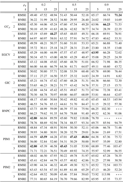
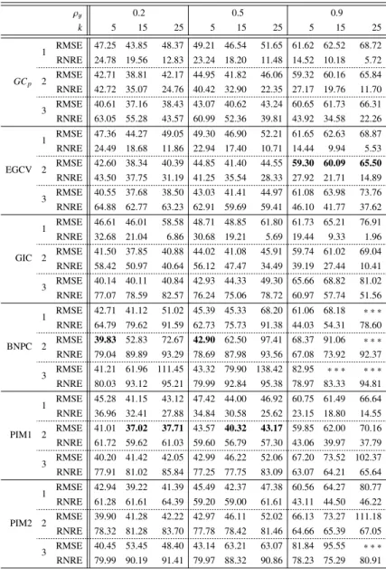
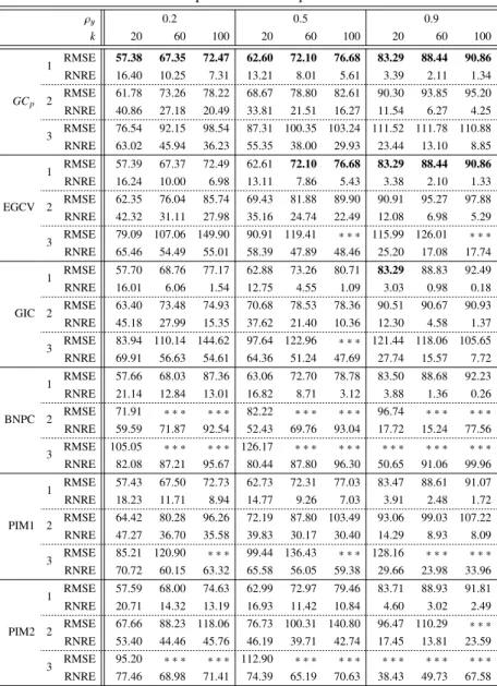
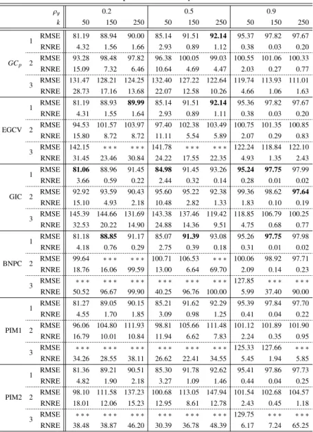
The remainder of the paper is organized as follows. In Section 2, we describe the MGR es- timator and MSCs for optimizing ridge parameters, and define a MSC class. In Section 3, we extend the algorithm proposed by Ohishiet al.(2020a) to optimize ridge parameters in MGR regression by the MSC minimization method. In Section 4, the MSC class defined in Section 2 is extended, corresponding to various distances. Moreover, we propose an algorithm for minimizing the extended MSC. In Section 5, we propose a new method for optimizing ridge parameters by using MSCs. In Section 6, we describe the MAL estimator and an equivalence between the MGR and MAL estimators under the regularization parameters optimized by the MSC minimization method. In Section 7, the performance of the ridge parameters optimized by the MSC minimization methods is compared by simulation. Technical details are provided in the Appendix.
2. Preliminaries
By a singular value decomposition,n×nandk×korthogonal matricesP andQand ak×k diagonal matrixD=diag(d1, . . . ,dk) expressXas
X=P
D1/2 On−k,k
Q′=P1D1/2Q′, (2.1) where On,k is an n×k matrix of zeros, P1 is ann×kmatrix obtained from the partition P = (P1,P2), which satisfiesP1′1n =0kandP1′P1 =Ik, andd1, . . . ,dkare eigenvalues of M (=X′X) satisfyingd1 ≥ · · · ≥dk>0. Then, the MGR estimators ofµandΞare given by
ˆ
µ=y¯, Ξˆθ=Mθ−1X′Y (Mθ=M+QΘQ′), (2.2) whereθ=(θ1, . . . , θk)′,Θ=diag(θ1, . . . , θk) andθj∈R+={θ∈R|θ≥0}(j=1, . . . ,k) is a regularization parameter called a ridge parameter. SinceMθ=Mwhenθ=0k, ˆΞθcoincides with ˆΞin (1.2) whenθ =0kand the MGR estimators coincide with the GR estimators when p =1. The MGR estimators in (2.2) denote the minimizers of the following penalized RSS (PRSS):
tr
(Y −1nµ′−XΞ)′(Y −1nµ′−XΞ)+Ξ′QΘQ′Ξ . (2.3) Although the ridge parameters adjust the amount of shrinkage of the MGR estimator ofΞ, since they are unknown, their optimization is an important task to obtain a better estimator. To simplify calculation, following Yanagihara (2018) and Ohishiet al.(2020a), we transform the ridge parameters as
δj= θj
dj+θj
∈[0,1] (j=1, . . . ,k).
Since this transformation is a one-to-one correspondence, the optimization ofθjis equal to that ofδj. Hence, we optimizeδjinstead ofθjand we also callδja ridge parameter in this paper.
Letδand∆be ak-dimensional vector and ak×kdiagonal matrix of the ridge parameters defined byδ=(δ1, . . . , δk)′and∆=diag(δ1, . . . , δk), respectively, and letZbe ak×pmatrix defined by
Z=(z1, . . . ,zk)′=P1′Y. (2.4)
Then, the MGR estimator ofΞin (2.2) can be rewritten as
Ξˆδ=Q(Ik−∆)D−1/2Z=Ξˆ −Q∆D−1/2Z. (2.5) In this paper, we optimize the ridge parameterδby using the MSC minimization method.
The MGR estimator in (2.5) gives a predictive matrix ofY as
Yˆδ=1nµˆ′+XΞˆδ =HδY, Hδ=Jn+P1(Ik−∆)P1′,
whereJn =1n1′n/nandHδ is ann×nmatrix called a hat matrix. Most MSCs consist of the predictive matrix and the hat matrix. The predictive matrix is used to evaluate model fit. We define an estimator and an unbiased estimator of the covariance matrixΣas
Σ(δ)ˆ =1
n(Y −Yˆδ)′(Y −Yˆδ), S= 1 b
Σˆ0
Σˆ0=Σ(0ˆ k), b=1−(k+1)/n
. (2.6) Under normality, ˆΣ(δ) is a penalized MLE ofΣand ˆΣ0is an MLE ofΣ. Then, model fit, i.e., the distance betweenY and ˆYδis defined by
trn
Σ(δ)Sˆ −1o .
On the other hand, the hat matrix is used to evaluate model complexity and it is defined by the following GDF:
df(δ)=ptr(Hδ). (2.7)
TheGCpand EGCV criteria for optimizing ridge parameters consist of tr{Σ(δ)Sˆ −1}and df(δ).
Similar to Yanagihara (2018), we have the following lemma about ˆΣ(δ) and df(δ).
Lemma 1. LetBδandW be p×p matrices defined by Bδ =Z′∆2Z, W =nΣˆ0.
Then,Σ(δ)ˆ anddf(δ)can be partitioned into terms which do and do not includeδas follows:
Σ(δ)ˆ = 1
n(W +Bδ)=Σˆ0+1 n
Xk j=1
zjz′jδ2j,
df(δ)=p(1+k)−ptr∆=p
(1+k)− Xk
j=1
δj
. From Lemma 1, we have
trn
Σ(δ)Sˆ −1o
=btr B∗δ
+bp, B∗δ=W−1/2BδW−1/2. Then, theGCpand EGCV criteria for optimizing ridge parameters are defined by
GCp(δ)=nbtr(Bδ∗)+nbp+αdf(δ), EGCV(δ)= btr(Bδ∗)+bp
{1−df(δ)/np}α,
whereαis a positive value adjusting the strength of the penalty for model complexity. Existing criteria are expressed by changing the value ofα, for example, theGCpand EGCV criteria co- incide with theCpand GCV criteria, respectively, whenα=2 and theGCpcriterion coincides with the MCp criterion (Yanagiharaet al., 2009) whenα = 2{1+(p+1)/(n−k−p−2)}. From the above, MSCs for optimizing ridge parameters can be regarded as bivariate functions of tr(B∗δ) and df(δ). Lemma 1 gives ranges of tr(Bδ∗) and df(δ).
Lemma 2. Thetr(Bδ∗)anddf(δ)are included in the following ranges:
tr(Bδ∗)∈
0,tr Z∗Z∗′, df(δ)∈[p,p(1+k)], whereZ∗=ZW−1/2.
Moreover, let f be a bivariate function defined by the following class.
Definition 1.(Class of the bivariate function f) For a positive valuer+,f satisfies the fol- lowing conditions:
(A1) For any (r,u)∈[0,r+]×[p,np), f(r,u) is continuous.
(A2) For any (r,u)∈[0,r+]×[p,np),f(r,u) is first order partially differentiable and its partial derivatives are positive.
We define MSC for optimizing ridge parameters by using f in Definition 4 as MSC(δ)=f
tr(B∗δ),df(δ)
. (2.8)
For theGCpand EGCV criteria, f is given by
f(r,u)=
fGCp(r,u)=nb(r+p)+αu (GCpcriterion) fEGCV(r,u)=b(r+p)/(1−u/np)α (EGCV criterion), andr+is given by
r+=tr Z∗Z∗′.
Then, the optimal ridge parameters based on minimizing the MSC in (2.8) are given by δˆ=(ˆδ1, . . . ,δˆk)′=arg min
δ∈[0,1]k
MSC(δ).
3. Fast Optimization of Ridge Parameters
In this section, to obtainδminimizing the MSC in (2.8), we extend the algorithm for op- timizing ridge parameters in the GR regression proposed by Ohishiet al.(2020a). First, we define the following class of ridge parameters.
Definition 2.(Class of ridge parameters) Forh ∈ R+, a class of ridge parameters is de- fined by
δ(h)ˆ =
δˆ1(h), . . . ,δˆk(h)′
, δˆj(h)=1−soft
1,h/z′jS−1zj ,
where zj is the p-dimensional vector defined by (2.4). Furthermore, soft(x,a) is a soft- thresholding operator (e.g., Donoho & Johnstone, 1994), i.e., soft(x,a) = sign(x)(|x| −a)+, and (x)+=max{x,0}.
WhenS =Ip andp =1, the class of ridge parameters in Definition 2 corresponds to that for the GR regression defined by Ohishiet al.(2020a). Using this class, the MGR estimator in (2.5) is given as a function ofh:
Ξˆδ(h)ˆ =QV(h)Q′Ξˆ,
whereQis thek×korthogonal matrix defined by (2.1) andV(h) is ak×kdiagonal matrix which has the following diagonal elements:
vj(h)=1−δˆj(h)=soft
1,h/z′jS−1zj
(j=1, . . . ,k). TheV(h) rewrites the predictive matrix ofY as
Yˆδ(h)ˆ =
Jn+P1V(h)P1′ Y,
whereP1 is then×kmatrix defined by (2.1). Then, the ridge parameters optimized by the MSC minimization method are given by the following theorem (the proof is given in Appendix A.1).
Theorem 1. We define r+as
r+=tr Z∗Z∗′.
For f with the class in Definition 4, letϕ(h) (h∈R+\{0})be a function defined by ϕ(h)=MSC( ˆδ(h)),
and suppose that∃ν >0s.t. ϕ(ν)<limh→0ϕ(h). Then, the ridge parameters optimized by the MSC minimization method are given byδ(ˆˆ h)andh is given byˆ
hˆ=arg min
h∈R+\{0}ϕ(h).
From this theorem, the class of ridge parameters in Definition 2 is the class of the “optimal”
ridge parameters.
Lettj(j=1, . . . ,k) be thejth order statistic ofz1′S−1z1, . . . ,z′kS−1zkandRj(j=0,1, . . . ,k) be a range defined by
Rj=
(0,t1] (j=0)
(tj,tj+1] (j=1, . . . ,k−1) (tk,∞] (j=k)
. (3.1)
Then, similar to Ohishiet al.(2020a), we have the following proposition.
Proposition 1. Theϕ(h)in Theorem 1 satisfies the following properties:
(P1) For all h∈R+\{0},ϕ(h)is continuous.
(P2) For all h≥tk,ϕ(h)= f(r+,p).
(P3) Theϕ(h)can be expressed as the following piecewise function:
ϕ(h)=ϕa(h)= f
(c1,a+c2,ah2)/nb,p(1+k−a−c2,ah)
(h∈Ra; a=0,1, . . . ,k), where c1,aand c2,aare nonnegative constants given by
c1,a=
0 (a=0)
Xa j=1
tj (a=1, . . . ,k), c2,a=
Xk j=a+1
1 tj
(a=0,1, . . . ,k−1)
0 (a=k)
.
From the results, the MSC minimization problem for optimizing ridge parameters in the MGR regression can be solved by applying the fast algorithm for the GR regression proposed by Ohishiet al.(2020a). That is, we have the following theorem.
Theorem 2. Suppose that the derivative ofϕa(h)in Proposition 1 is expressed as d
dhϕa(h)=χa(h)ψa(h) (h∈Ra; a=0,1, . . . ,k−1),
andψ(h)=ψa(h) (h∈Ra)is continuous for all h∈R+\{0}, whereχa(h)is a positive function andψa(h)is a polynomial. Moreover, suppose that∃ν >0 s.t. ϕ(ν)<limh→0ϕ(h)and let ha
be a root ofψa(h)=0satisfying
∃ϵa>0s.t.∀ϵ∈(0, ϵa), ψa(ha−ϵ)<0. (3.2) Then, minimizer candidates ofϕ(h)are given by
S=
[
a∈A
{ha}
[ T,
A={a∈ {0,1, . . . ,k−1} |ha∈Ra}, T =
{tk} (ψk−1(tk)<0)
∅ (ψk−1(tk)≥0).
Hence, the ridge parameters optimized by the MSC minimization method are given byδ(ˆˆh)and h is given byˆ
hˆ =arg min
h∈Sϕ(h).
Although the range ofhis a set of positive values, Theorem 2 can reduce a search range ofhto Swhich is a set of discrete points. Furthermore, each element ofSis given as closed form and
#(S)≤k+1; hence we can quickly optimize the ridge parameters. In the theorem, although ψa(h) is implicitly supposed as a linear or quadratic function, the theorem can naturally be ex- tended to higher order polynomial functions. In particular, roots ofψa(h)=0 can be obtained as closed forms whenψa(h) is a cubic or a quartic function, by using Cardano’s formula (e.g., David, 2004, Chap. 1) or Ferrari’s method (e.g., Tignol, 2001, Chap. 3). Hence, if the degree ofψa(h) is four or less, we can quickly optimize the MSC.
3.1. Examples
In this subsection, we provide specific examples of the MSC minimization methods for optimizing ridge parameters in the MGR regression. To emphasize that the optimal ridge pa- rameters depend onα, we specify thatαis given.
3.1.1. TheGCpcriterion
Although the ridge parameters optimized by theGCp criterion minimization method have already been given by Nagai et al.(2012), here we show how to derive them by applying Theorem 2. TheGCpcriterion for optimizing ridge parameters is given by
GCp(δ|α)=fGCp
tr(B∗δ),df(δ) α . Whenh∈Ra(a=0,1, . . . ,k),ϕand its derivative are given by
ϕ(h|α)=ϕa(h|α)=c2,ah2−αpc2,ah+nbp+c1,a+αp(1+k−a), d
dhϕa(h|α)=c2,a(2h−αp).
Hence, the ridge parameters optimized by theGCpcriterion minimization method are given as the following closed form:
δˆ=δ(ˆˆ hα), hˆα=αp 2 .
3.1.2. The EGCV criterion
The EGCV criterion for optimizing ridge parameters is given by EGCV(δ|α)= fEGCV
tr(B∗δ),df(δ) α . Whenh∈Ra(a=0,1, . . . ,k),ϕand its derivative are given by
ϕ(h|α)=ϕa(h|α)=bp+(c1,a+c2,ah2)/n {b+(a+c2,ah)/n}α , d
dhϕa(h|α)= c2,a
n2{b+(a+c2,ah)/n}α+1ψa(h|α),
ψa(h|α)=−(α−2)c2,ah2+2(a+nb)h−α(nbp+c1,a). Whenα=2, i.e., using the GCV criterion minimization method, we have
ψa(h|2)=2{(a+nb)h−nbp−c1,a}, and a root ofψa(h|2)=0 is
ha= nbp+c1,a
a+nb .
Moreover, similar to Yanagihara (2018), the following statement is true:
∃!a∗∈ {0,1, . . . ,k−1}s.t.ha∗∈Ra∗.
Hence, the ridge parameters optimized by the GCV criterion minimization method are given by the following closed forms: ˆδ=δ(hˆ a∗).
Whenα > 2, sinceψa(h | α) is a concave quadratic function, a root of ψa(h | α) = 0 satisfying the condition (3.2) is given by
hα,a= (a+nb)−p
(a+nb)2−α(α−2)c2,a(nbp+c1,a)
(α−2)c2,a .
Therefore, candidates of ˆhαare given by Sα=
[
a∈Aα
{hα,a}
[ Tα,
whereAαandTαare sets given by Aα=
a∈ {0,1, . . . ,k−1} |hα,a∈Ra , Tα =
{tk}
r+>2(1−n−1)tk/αb−p
∅
r+≤2(1−n−1)tk/αb−p. Hence, the ridge parameters optimized by the EGCV criterion minimization method are given by
δˆ=δ(ˆˆ hα), hˆα=arg min
h∈Sαϕ(h|α).
In the EGCV criterion minimization method, the number of minimizer candidates is onlyk+1 at most.
3.2. Relationships between the Optimal Ridge Parameters
This subsection provides some theoretical properties concerning the relationships between the optimal ridge parameters. The class of the optimal ridge parameters satisfies
∀h1,h2∈R+,h1<h2⇒δˆj(h1)≤δˆj(h2) (j=1, . . . ,k),
with equality only when h1 ≥ tk. This fact yields some relationships concerning the ridge parameters optimized by theGCpand EGCV criteria minimization methods. Immediately, we have the following result which is similar to Nagaiet al.(2012).
Proposition 2. For positive valuesα1 andα2, we define the ridge parameters optimized by the GCpcriterion minimization method as
δˆ1,j=δˆj(ˆhα1), δˆ2,j=δˆj(ˆhα2) (j=1, . . . ,k), wherehˆα =αp/2. Then, we have
α1< α2⇒δˆ1,j≤δˆ2,j.
This proposition states that the stronger the penalty for model complexity, the larger the amount of shrinkage of the estimator, when using theGCp criterion minimization method. Next, we consider the ridge parameters optimized by theGCpand the GCV criteria minimization meth- ods. Similar to Yanagihara (2018), we have the following lemma.
Lemma 3. The ha∗obtained by the GCV criterion minimization method satisfies ha∗ ≤p.
This lemma leads to the following result which is similar to the case whenp=1 (Yanagihara, 2018).
Proposition 3. LetδˆGCα,jp andδˆGCVj (j = 1, . . . ,k)be the ridge parameters optimized by the GCpand GCV criteria minimization methods, respectively. Then, we have
α≥2⇒δˆGCVj ≤δˆGCα,jp.
The value ofαin the MSC is often 2 or more. This means that the ridge parameters optimized by theGCpcriterion minimization method shrink the estimator more than the GCV criterion minimization method in most cases. Finally, we consider the ridge parameters optimized by the EGCV criterion minimization method. We expressϕ(h|α)=EGCV( ˆδ(h)|α) as
ϕ(h|α)=σˆ2(h)η(h|α), where
σˆ2(h)=bp+btr(Bδ∗), η(h|α)= 1
{1−df(h)/np}α, df(h)=df( ˆδ(h)),
and let ˆhαbe the minimizer ofϕ(h|α). Then,η(h|α) has the following property (the proof is given in Appendix A.2).
Lemma 4. Suppose that0<h1<h2. Then, we have η(h2|α)≤η(h1|α).
This lemma leads to the following proposition (the proof is given in Appendix A.3).
Proposition 4. The EGCV criterion minimization method has the following properties:
(1) Suppose thatα1< α2. Then, we have
hˆα1=tk⇒hˆα2=tk.
(2) For positive valuesα1 andα2, we define the ridge parameters optimized by the EGCV criterion minimization method as
δˆ1,j=δˆj(ˆhα1), δˆ2,j=δˆj(ˆhα2) (j=1, . . . ,k), and suppose thathˆα2 ,tk. Then, we have
α1< α2⇒δˆ1,j≤δˆ2,j, with equality only whenhˆα1 ≥z′jS−1zj.
This proposition states that the stronger the penalty for model complexity, the larger the amount of shrinkage of the estimator, when using the EGCV criterion minimization method.
4. Extending the MSC Class
In the previous section, we showed that the algorithm for the GR regression can be applied to minimize the MSC in (2.8), where the distance betweenY and ˆYδis defined by tr{Σ(δ)Sˆ −1} and the MSC is defined by using tr(Bδ∗) obtained from the distance. In this section, we focus on how to measure the distance.
Letgbe a real-valued function defined by the following class.
Definition 3.(Class of the functiong) For anyp×ppositive definite matrixA, thegsat- isfies the following conditions:
(A1) Theg(A) is positive.
(A2) The∂g(A)/∂Ais a positive definite.
Using the functiong, we extend the MSC in (2.8) to MSC(δ|g)= f
g(Bδ∗),df(δ)
, (4.1)
where f is the bivariate function given by Definition 4. For example,gincludes the following functions:
g(A)=
gLH(A)=tr(A) (LH-distance)
gLR(A)=logIp+A (LR-distance)
gBNP(A)=trn
A(Ip+A)−1o
(BNP-distance) gML(A)=trn
(Ip+A)−1o
+log|Ip+A| −p (ML-distance) gGLS(A)=tr(A2)/2 (GLS-distance)
.
The MSC in (4.1) is equal to that in (2.8) wheng(A) =gLH(A) and the following equation holds:
gLH(Bδ∗)=tr
BδW−1 .
Since we can regardBδ as a between-group variation matrix andW as a within-group varia- tion matrix,gLH(B∗δ) is a Lawley-Hotelling trace criterion (LH-statistic; e.g., Anderson, 2003, Chap. 8) which is a well-known statistic in multivariate analysis. That is, the MSC in (2.8) measures the distance betweenY and ˆYδ based on the LH-statistic. Similarly, regarding the LR-distance and the BNP-distance, the following equations hold:
gLR(Bδ∗)=log(W +Bδ)W−1, gBNP(Bδ∗)=trn
Bδ(W +Bδ)−1o .
They are a Likelihood-Ratio criterion and a Bartlett-Nanda-Pillai trace criterion, respectively, which are also well-known statistics (e.g., Anderson, 2003, Chap. 8). MSC based on the LR- distance includes the GIC and the AICCunder normality. The above three distances based on the three statistics pertain to the mean structure of a model. In contrast, there are distances with respect to the covariance structure of a model, e.g., the ML-distance and the GLS-distance. Re- garding these distances, the following equations hold:
gML(B∗δ)=logΣ(δ)ˆ +trn
Σ(δ)ˆ −1Σˆ0
o−logΣˆ0−p, gGLS(B∗δ)=1
2trn
Σˆ0−Σ(δ)ˆ Σˆ−01o2
.
They are distances between ˆΣ(δ) and ˆΣ0 called a maximum likelihood fitting function and a generalized least square fitting function, respectively (e.g., Bollen, 1989, Chap. 4). Using g(A), theGCpand EGCV criteria, and the GIC and the AICCunder normality are given by
GCp(δ)=nbgLH(Bδ∗)+nbp+αdf(δ), EGCV(δ)= bgLH(Bδ∗)+bp
{1−df(δ)/np}α,
GIC(δ)=ngLR(Bδ∗)+nplogb+αdf(δ), AICC(δ)=ngLR(Bδ∗)+nplogb+ np{n+df(δ)}
n−p−1−df(δ).
Using the GIC, it is also possible to adjust the strength of the penalty for model complexity, and for example, the GIC coincides with the AIC whenα =2, the HQC (Hannan & Quinn, 1979) whenα =2 log logn, and the BIC (Schwarz, 1978) whenα =logn. For the GIC and AICC, the bivariate functionf(r,u) is given by
f(r,u)=
fGIC(r,u)=n(r+plogb)+αu (GIC) fAICC(r,u)=n(r+plogb)+ np(n+u)
n−p−1−u (AICC). The following subsections describe two algorithms to minimize the MSC in (4.1).
4.1. Minimizing MSC via Iterative Method
This subsection describes an algorithm for solving the MSC minimization method via an iterative method with an iterative function. That is, we derive the iterative function. Notice that
Bδ∗ = Xk
j=1
z∗jz∗j′δ2j, z∗j =W−1/2zj.
Therefore, the following partial derivatives can be obtained:
∂
∂δj
Bδ∗=2z∗jz∗j′δj, ∂
∂δj
df(δ)=−p. We express the (i, ℓ) element of a matrixAasaiℓ =(A)iℓand define
g˙iℓ(B)= ∂
∂aiℓg(A)A=B, G(B)˙ = ∂
∂Ag(A)A=B. Bδ∗is a symmetric matrix, thus we have
∂
∂δjg(Bδ∗)= Xp
i=1
Xp ℓ=i
∂
∂δj
(Bδ∗)iℓ·g˙iℓ(Bδ∗)=2z∗j′G(B˙ δ∗)z∗jδj. Hence, a partial derivative of the MSC is given by
∂
∂δj
MSC(δ|g)=2z∗j′G(B˙ δ∗)z∗jf˙r
g(B∗δ),df(δ)
δj−pf˙u
g(Bδ∗),df(δ) ,
where
f˙r(x, y)= ∂
∂rf(r,u)(r,u)=(x,y), f˙u(x, y)= ∂
∂uf(r,u)(r,u)=(x,y). By solving∂MSC(δ|g)/∂δ=0k, we can obtain the following iterative method:
δ(i+1)=ζ(δ(i))=
ζ1(δ(i)), . . . , ζk(δ(i))′
(i=0,1, . . .), ζj(δ)=1−soft
1, τ(δ)/z∗j′G(B˙ δ∗)z∗j
, (4.2)
where (i) is the iteration number,δ(0)is a given initial vector, andτ(δ) is given by τ(δ)= pf˙u
g(Bδ∗),df(δ) 2 ˙fr
g(Bδ∗),df(δ) >0.
By repeating the update ofδ(i)with the iterative functionζ, we can obtain the optimalδ. This iterative method has the following property (the proof is given in Appendix A.4).
Proposition 5. For a k-dimensional vectorϵwherein all elements are nonnegative, suppose that
τ(δ)≤τ(δ+ϵ), z∗j′G(B˙ ∗δ)z∗j ≥z∗j′G(B˙ ∗δ+ϵ)z∗j. (4.3) Then, the iterative method with iterative function(4.2)converges if∀j∈ {1, . . . ,k}, δ(1)j ≥δ(0)j . Furthermore, the iterative method also converges if∀j∈ {1, . . . ,k}, δ(1)j ≤δ(0)j .
From this proposition, when assumption (4.3) holds, the iterative method with iterative func- tion (4.2) converges if the initial vector is0kor1k.
4.1.1. LR-distance
For the MSC based on the LR-distance, the following equation holds:
∂
∂AgLR(A)= ∂
∂Alog|Ip+A|=(Ip+A)−1. Therefore, we have
W−1/2G(B˙ ∗δ)W−1/2=(W +Bδ)−1=1 n
Σ(δ)ˆ −1.
Hence, the iterative function for solving the MSC minimization method based on the LR- distance is given by
ζj(δ)=1−soft
1,nτ(δ)/z′jΣ(δ)ˆ −1zj
. (4.4)
Furthermore, from Lemma 1, forϵin Proposition 5 and for any p-dimensional vectora, the following equation holds:
a′Σ(δ)aˆ ≤a′Σ(δˆ +ϵ)a⇐⇒a′Σ(δ)ˆ −1a≥a′Σ(δˆ +ϵ)−1a.
Let ˆδLRbe a solution obtained by the iterative method with iterative function (4.4). Then, δˆLR=ζ( ˆδLR).
The ridge parameters optimized by the MSC minimization method based on the LR-distance are given by
δˆLRj =1−soft
1,nτ( ˆδLR)/z′jΣ( ˆˆ δLR)−1zj
(j=1, . . . ,k).
On the other hand, the ridge parameters optimized by the MSC minimization method based on the LH-distance are given by the following form:
δˆLHj =1−soft
1,hˆ/z′jS−1zj
(j=1, . . . ,k).
The ˆδLHj includesS−1andSis an estimator of the covariance matrix for the full model. Thus, δˆLHj has a disadvantage becauseS−1is unstable whenkis large. Whereas, ˆδLRj does not include S−1, but rather ˆΣ( ˆδLR)−1and ˆΣ( ˆδLR) is an estimator of the covariance matrix adjusted by ˆδLR. Thus, ˆδLRj has an advantage because ˆΣ( ˆδLR)−1is stable even whenkis large.
Example 1
We derive an iterative function for solving the GIC minimization method. From f(r,u) = fGIC(r,u), we have
f˙r(r,u)=n, f˙u(r,u)=α,
and therefore,τ(δ)=αp/2n. Hence, the iterative function for the GIC minimization method is given by
ζj(δ)=1−soft
1, αp/2z′jΣ(δ)ˆ −1zj
(j=1, . . . ,k). (4.5) Moreover, sinceτ(δ) does not depend onδ, from Proposition 5, the iterative method for solving the GIC minimization method converges under an appropriate initial vector.
Example 2
We derive an iterative function for solving the AICCminimization method. From f(r,u)= fAICC(r,u), we have
f˙r(r,u)=n, f˙u(r,u)= np(2n−p−1) (n−p−1−u)2, and therefore, we have
τ(δ)= p2(2n−p−1) 2{n−p−1−df(δ)}2.
Hence, the iterative function for the AICCminimization method is given by ζj(δ)=1−soft
1, np2(2n−p−1) 2{n−p−1−df(δ)}2z′jΣ(δ)ˆ −1zj
(j=1, . . . ,k). Moreover, forϵin Proposition 5, the following equation holds:
df(δ)≥df(δ+ϵ). Therefore
τ(δ)≥τ(δ+ϵ),
and thus, the iterative method for solving the AICC minimization method does not satisfy Proposition 5.
4.1.2. BNP-distance
For the MSC based on the BNP-distance, the following equation holds:
∂
∂AgBNP(A)= ∂
∂Atrn
A(Ip+A)−1o
=− ∂
∂Atrn
(Ip+A)−1o
=(Ip+A)−2. Therefore, we have
W−1/2G(B˙ ∗δ)W−1/2=(W +Bδ)−1W(W +Bδ)−1= 1
nΣ(δ)ˆ −1Σˆ0Σ(δ)ˆ −1.
Hence, the iterative function for solving the MSC minimization method based on the BNP- distance is given by
ζj(δ)=1−soft
1, nτ(δ) z′jΣ(δ)ˆ −1Σˆ0Σ(δ)ˆ −1zj
.
Accordingly, using the BNP-distance, the optimal ridge parameters are stable even whenkis large.
Example
As an example of MSC based on the BNP-distance, we consider the following criterion:
BNPC(δ)=ngBNP(Bδ∗)+αdf(δ). Then, since
f˙r(r,u)=n, f˙u(r,u)=α,
we have τ(δ) = αp/2n. Hence, the iterative function for solving the BNPC minimization method is given by
ζj(δ)=1−soft
1, αp
2z′jΣ(δ)ˆ −1Σˆ0Σ(δ)ˆ −1zj
. (4.6)
4.1.3. ML-distance
For the MSC based on the ML-distance, the following equation holds:
∂
∂AgML(A)= ∂
∂A htrn
(Ip+A)−1o
+log|Ip+A|i
=−(Ip+A)−2+(Ip+A)−1. Therefore, we have
W−1/2G(B˙ δ∗)W−1/2=(W +Bδ)−1−(W +Bδ)−1W(W +Bδ)−1
= 1 n
Σ(δ)ˆ −1−1 n
Σ(δ)ˆ −1Σˆ0Σ(δ)ˆ −1.