This paper analyzes the life-cycle medical expenditure risks of individuals and the roles of the national health insurance system using nationwide administrative data of health insurance claims (NDB) in Japan. Each of the dimensions of heterogeneity plays a role in estimating the heterogeneous effects of risks of medical expenditures and insurance programs. Nakajima and Telyukova (2018) and Kopecky and Koreshkova (2014) also study the interaction of medical expenditure risks and elderly savings.
In the next section, we exploit panel characteristics of the NDB data and examine the persistence of individuals' medical expenditures over various time periods. 2018) use the data from the Japan Medical Data Center (JMDC) and analyze the persistence of individuals' medical expenditures. As an example, Table 2 shows distribution of the health status in the next period,ht+1, conditional on poor health status in the current period,ht.
Lifetime Medical Expenditures
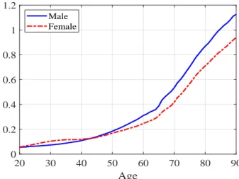
As shown in Figure 1, average expenditure is higher for men than for women except for a few years in the late 20s and early 30s, but average lifetime expenditure is higher for women than for men due to longer life expectancy. Table 3 also lists the higher moments, and there is considerable heterogeneity in the total health expenditure that we would face over the life cycle, which is not surprising given the persistent and large expenditure shocks studied in Section 2.3. For the M(1) process, for example, we ignore the health status data in the past period.
Standard deviations of male lifetime expenditure, as shown in the second row of the table, decrease from 10.9 million yen when we assume an M(2) process to 9.8 million yen with M(1), 7.6 million with i.i.d. In the deterministic case, the expenditure at each age is the same for everyone, and the distribution is only associated with mortality risks. Coefficients of variation also move in the same direction, as means are essentially the same across specifications.
The second-order Markov process would imply most of the population in the group with the lowest lifetime expenditures of less than 10 million yen, as well as a group with the largest expenditures of more than 40 million yen. 7A deterministic case is not included in the figure, because the distribution depends only on the time of death and is very irregular with high peaks. Furthermore, healthier individuals who survive long in the baseline M(2) are assumed to die sooner in the counterfactual experiment.
Risks are also much greater, and the coefficients of variation will be 0.72 and 0.60 for males and females respectively under the experiment and they are much higher than 0.53 and 0.48 in the baseline model. As shown in the last two rows of Table 6, there would be many more individuals in the lower and upper tails of the distribution under the experiment, as also visualized in Figure 10.
3 The Model
- Demographics
- Marital Status
- Health Status and Medical Expenditures
- Preferences and Endowment
- Government
- Households’ Problem
An individual of skill is matched with a spouse of skill′ with probabilityνs,s′, which accounts for educational assortative mating. We denote by h the health status of an individual and assume that medical expenses and survival probabilities depend on the health status. In our baseline model, it is a vector containing information about an individual's health status in the current and previous periods, h = {h, h−1}.
The law of movement of health status is denoted as ∼ ∼fh(j, g,h) and depends on an individual's age and sex. We assume that individuals have warm-hearted bequest motives and that they derive utility from leaving bequests, denoted as χ(a′), where a' denotes the assets an individual leaves when he dies. Labor supply is exogenous and earnings of an individual depend on age j, gender, skills and marital status ζ.
The out-of-pocket medical expenses paid by an individual are limited by a ceiling, denoted as m, which depends on an individual's age and income. Out-of-pocket expenses paid by an individual are referred to as mop and given as:. Value function of singles S: The state vector of a single individual is given as (j, g, s, a,h), where j indicates age, g gender, s skill, a asset and h health status.
Given the states, an individual optimally chooses consumption and savings a′ to maximize utility over the life cycle. The new value function M has a state vector that includes the health status and skill of the spouse and the assets of the married couple will be a′ +a, where the second term a indicates the assets of the spouse to which the individual matches.
4 Calibration
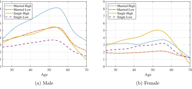
They correspond to the bottom 50% of the distribution of medical expenses within each group, the next 30% (from 51 to 80 percentiles), 15%. 17We used the ESS data from 2017, provided as order data from the Statistics Bureau of the Ministry of Interior and Communications (MIC). What is striking is that the order of the four profiles is very different between men and women.
For details about the program, see the description on the website of the Ministry of Health, Labor and Welfare. Expenditure data are taken from the Statistics of Long-term Care Benefit Expenditures in the Ministry of Health, Labor and Welfare (MHLW).19 They report total expenditure on different types of long-term care benefits broken down by gender and age group. We combine this and demographic data and calculate average long-term care costs by age and sex.
Note: The figure shows the average gross expenditures for long-term care of all individuals by age and gender in 2015. Data on expenditures are from the Statistics of Expenditures for Long-Term Care of the Ministry of Health, Labor and Social Welfare (MZDS). Population data are from the population statistics of the National Institute for Population and Social Security Research (IPSS).
The pension replacement rate κ is set at one third, based on an estimate of the average gross replacement rate of public pensions from the OECD (2019). 20 The amount is set to be in the range of the average payments of the Public Assistance program (seikatsu hogo) according to family size.
5 Numerical Analysis
- Baseline Model
- Roles of Health Insurance
- Alternative Specification of Medical Expenditure Risks
- Alternative Model Specifications
We also assess the role of the means-tested welfare program and its interaction with health expenditure risk and the health insurance system. First, we assume that no health insurance is provided and that individuals are responsible for all medical expenses. The bottom panels of Figure 23 highlight the differences in the effects of poor health in the two economies with and without health insurance.
The bottom panels show the difference in the top panel after subtracting assets and consumption from households in excellent health from households in poor health. We assume the same medical expenditure process and health insurance as in the base model first, but will consider different scenarios later. We now consider the same extreme scenario of eliminating health insurance in economies with these two different welfare programs.
The results are summarized in Table 12, where the comparison is relative to the basic model with a different value of the consumption threshold c, and the changes represent the effects of removing health insurance in the regime. The loss of social welfare due to the loss of health insurance is much greater in such an economy, as shown in the lower part of the table. In the basic model, 16.2% of total expenditures are paid by households as out-of-pocket expenditures, while the rest, 83.8%, is paid by health insurance and the state.
We then compare the effects of removing health insurance under the three specifications, and the results are summarized in Table 15. Comparison is relative to a baseline model with a different medical expenditure process, and changes represent the effects of removing health insurance in each economy. In Table 16, we compare the effects of removing health insurance where people face deterministic but heterogeneous life-cycle costs of medical expenses.
Individuals who experience persistent bad health shocks suffer from large health expenditures and are likely to be enrolled in a welfare program without health insurance.

6 Conclusion
Note: The first column shows the changes relative to the baseline model with health-independent earnings, while the second column shows the effects of raising the surcharge rates to 30% in the health-independent earnings economy. The line "Recipients of transfers" indicates the share of the population receiving social transfers in each experiment. The percentage change in the number of recipients compared to the base model is given in parentheses.
Our model incorporates details of the national health insurance system in Japan, including age-dependent copayment rates and progressive ceilings on out-of-pocket expenditures through high-cost medical expense benefits. We show that the health insurance system protects Japanese individuals well from expenditure risks and significantly affects saving behavior. Households with higher lifetime incomes, including high-skilled singles and married couples, will increase savings by significantly more, but low-income individuals such as low-skilled single women will see savings reduced and be more likely to become recipients of income-tested transfers. .
Low-income households face greater fluctuations in their assets and consumption in response to medical spending shocks, and the welfare effects of losing insurance are more negative than those of high-income households. The welfare effects, when revenues are redistributed in the form of a lump sum transfer and the government budget is balanced, are positive on average, but the effects are lower or more negative for households with lower incomes and poor health shocks. We also show that the economic and welfare effects of health care reform depend on the generosity of wealth transfer programs, and that this occurs in different ways across different households.
In this paper we focus on the effects of medical spending and insurance programs in a demographically stationary economy and abstract from the effects of demographic change. Demographic trends facing Japan and countries around the world, including increasing life expectancy, declining birth rates, and changing family structures, may interact with the economic and welfare evaluations of alternative policy reforms related to medical spending, which we leave for future research.
Health Insurance Reform - The Impact of the Medicare Purchase. Journal of Economic Dynamics and Control. Uncertain medical costs and precautionary savings at the end of the life cycle. Review of Economic Studies.


