Firm-to- rm Trade in Sticky Production Networks

Firm-to-rm Trade in Sticky Production Networks

Kevin Lim

January 2018

Abstract

This paper develops a structural model of trade between heterogeneous rms in which the network of rm-level input-output linkages is determined both dynamically and endogenously. Firms vary in the size of their customer and supplier bases, occupy heterogeneous positions in dierent supply chains, and adjust their sets of trade partners over time. Despite the rich heterogeneity and dynamics, the model remains computa- tionally tractable. Using both cross-sectional and panel data on trading relationships between US rms, I estimate the model's key parameters via a simulated method of moments technique and assess its t to the data. Simulations of the model are then used to study how the structure and dynamics of the production network matter for the propagation of rm-level supply and demand shocks and their translation into aggregate eects.

∗[email protected]. I am extremely grateful to Gene Grossman, Steve Redding, and Esteban Rossi- Hansberg for their support and guidance in writing this paper. I also thank Oleg Itskhoki, Ezra Obereld, Davin Chor, as well as numerous seminar participants and visiting faculty at Princeton University for helpful discussions and comments. Later drafts of this paper beneted enormously from feedback and comments during the job market at numerous seminars, as well as from discussions with the trade communities at Dartmouth College and the University of Toronto. This research beneted from nancial support from the International Economics Section at Princeton University.

1 Introduction

Many of the goods and services that are traded between rms lack centralized markets or intermediaries facilitating their exchange, and instead are traded through direct connections between buyers and sellers.¹ Firm-level supply and demand shocks propagate via these connections, through the network of rm-to-rm relationships, and translate into aggregate eects. The nature of this propagation depends in principle on several empirically stark features of the production network that are often abstracted from in existing theories of production. First, rms vary in the extent to which they are connected to other rms (relationship heterogeneity). Second, rms occupy dierent positions in dierent supply chains (supply chain heterogeneity). Third, the set of active trading relationships changes over time (relationship dynamics). In this paper, I study the extent to which accounting for these characteristics of the production network matters for our understanding of rm-level supply and demand shock propagation.

To do so, I rst develop a structural model of trade between heterogeneous rms in which the network of rm-level input-output linkages is endogenously determined. In the model, active relationships face a time-varying cost, and frictions impede the ability of forward- looking rms to change their sets of trade partners. These assumptions deliver a model of a production network where rms vary in the size of their customer and supplier bases, occupy heterogeneous positions in dierent supply chains, and adjust their sets of active relationships dynamically. I develop tractable computational algorithms to solve for the model's steady-state as well as its transition dynamics, and use both cross-sectional and panel data on rm-level trading relationships in the US to estimate the model's key parameters via a simulated method of moments technique. Finally, simulations of the model are used to study how relationship heterogeneity, supply chain heterogeneity, and relationship dynamics matter for the aggregate welfare eects of shocks to rm-level productivity and demand.

The key ndings of the analysis are as follows. First, accounting for the heterogeneous distribution of relationships leads to lower predicted welfare eects of shocks to small rms, and larger predicted eects of shocks to large rms. This results intuitively from the fact that large rms are central to the production network not only because they are large in size, but also because they are more connected to other rms in the economy than smaller rms. Second, if one takes the production network as xed, the higher-order propagation of rm-level shocks multiple stages upstream or downstream of supply chains appears to be quantitatively unimportant. In the simulations studied, over 90% of the short-run welfare

1Using the Rauch (1999) classication of products, for example, only about15% of trade by US rms in 2014 was in goods that have organized exchanges, while another 15% was in goods that have reference prices (implying the existence of specialized traders engaging in price arbitrage).

eects of rm-level shocks are accounted for by propagation one stage upstream or down- stream of where the shock hits. Third, it is the dynamic propagation of rm-level shocks that is quantitatively important instead, as the predicted welfare eects can dier dramatically once the endogenous adjustment of the network is taken into account.

In modeling the dynamics of rm-level trading relationships, this paper is most closely related to the models of Obereld (2015) and Chaney (2014, 2015). In both of these models, as in this paper, the network of rm-level input-output linkages is an endogenous and dyna- mic outcome of a stochastic process by which potential buyer-supplier pairs receive trading opportunities over time. In Obereld (2015), however, the number of suppliers per rm is exogenously xed, while in Chaney (2014, 2015), every rm has the same number of suppliers even though the number of suppliers per rm grows over time. Relationship heterogeneity is therefore shut down in these models.

In modeling the matching between buying and selling rms, this paper is also closely related to the models of Bernard, Moxnes, and Saito (2015) and Bernard, Moxnes, and Ulltveit-Moe (2015). In both of these models, variation in the extensive margin of rm-to- rm relationships is similarly generated by assuming that relationships are costly. However, these papers address the static formation of relationships between one group of buyers and one group of sellers, in essence capturing one tier of relationships between rms instead of the entire network. Supply chain heterogeneity and relationship dynamics are therefore absent in these models.

In addition, this paper builds on the existing literature studying how microeconomic shocks translate into aggregate uctuations. Acemoglu et al (2012) argue that the network structure of linkages between sectors matters for how idiosyncratic sector-level shocks trans- late into aggregate movements, while Magerman et al (2016) make an analogous argument by studying the production network between rms. However, neither of these papers seeks to explain what determines the network structure of the economy in the rst place, nor how the network structure evolves in response to changes in the economic environment. The theory developed in this paper endogeneizes the formation of the production network, and therefore allows us to address these questions.

In this last regard, the theory developed here is related to the broader theoretical lite- rature on social and economic network formation, within which there are two qualitatively dierent approaches to modeling the formation of ties between atomistic agents.² The rst approach posits an exogenous stochastic algorithm for the formation of links, and then pro- ceeds to study the resulting network properties.³ As these models of network formation

2See Jackson (2005, 2011) for more in-depth surveys of the network formation literature.

3Well-known examples from the graph theory literature are the Erdös-Rényi (1959) random network, the

are non-structural, however, they cannot be used to study how networks of trade between rms respond to changes in economic incentives. The second approach to modeling network formation assumes that the creation and destruction of links are the result of strategic in- teractions between agents.⁴ These game-theoretic approaches therefore explicitly take into account optimizing behavior by the agents constituting the network, but the complexity of solving these models beyond simple illustrative examples precludes quantitative analysis.

The modeling of network formation in this paper can thus be viewed as a combination of the two approaches discussed above, or in the terminology of Currarini, Jackson, and Pin (2010), a combination of chance and choice: rms receive the opportunity to adjust relationships according to an exogenous stochastic process, but the activation or termination of a trading relationship conditional on having the opportunity to do so is an endogenous outcome. This hybrid approach is similar in spirit to the dynamic network formation models in Bala and Goyal (2000), Watts (2001), and Jackson and Watts (2002), but within the context of a structural model of trade between heterogeneous producers that can be used for quantitative analysis.⁵

The outline of this paper is as follows. I begin in section 2 by developing a static version of the theoretical model, in which the set of buyer-supplier relationships is taken as given.

I characterize how rm size, rm-to-rm trade volumes, and aggregate outcomes such as household welfare depend on the existing production network, and show how to solve for the market equilibrium of the model given any network of relationships. In section 3, I then endogeneize the formation of linkages between rms in the economy by introducing a dynamic matching process between potential buyers and sellers, and discuss how to solve for both the model's steady-state as well as its transition dynamics. In section 4, I discuss the data used for structural estimation of the model's parameters, the simulated method of moments estimation approach, and the t of the model to data. Section 5 then discusses the simulation exercises, and section 6 concludes.

Watts-Strogatz (1998) small world model, and the Barabási-Albert (1999) preferential attachment model.

In the economics literature, Atalay et al (2011) combine the random and preferential attachment algorithms to model the buyer-supplier network in the US economy.

4Aumann and Myerson (1988) and Myerson (1991) model network formation as extensive-form and simultaneous move games respectively. Jackson and Wolinsky (1996) adopt a cooperative game theoretic approach, while Kranton and Minehart (2001) study buyer-seller networks in which ascending-bid auctions are used to determine the formation of links.

5Bala and Goyal (2000), Watts (2001), and Jackson and Watts (2002) also assume for tractability that agents are myopic in their decisions about which links to form, whereas rms in this paper are forward-looking and optimally select relationships taking into account their future costs and benets.

2 Static Model

To study the dynamic formation of rm-to-rm linkages, it is useful to rst understand how rms behave conditional on these relationships. I therefore begin by describing a static version of the model in which the network of trading relationships between rms is xed.

2.1 Model environment

The economy consists of a representative household and an exogenously-given unit con- tinuum of rms that each produce a unique good. Firms are heterogeneous over states χ= (φ, δ), whereφandδ are what are referred to as the fundamental productivity of a rm's production process and the fundamental demand for a rm's product respectively. The exo- genous cumulative distribution function over rm states is denoted by G_χ, with density g_χ and support S_χ a bounded subset of R²+.⁶ For brevity, I also refer to rms with state χ as χ-rms.

2.1.1 Households

The representative household supplies L units of labor inelastically and has constant- elasticity-of-substitution (CES) preferences over all goods in the economy, given by:

U =

"

Z

Sχ

[δx_H(χ)]^σ−1σ dG_χ(χ)

#_σ−1^σ

(2.1) Here, σ denotes the elasticity of substitution across varieties, and x_H(χ) is the household's consumption ofχ-rm varieties. Given the price p_H(χ)charged byχ-rms to the household, household demand is given by:

x_H(χ) = ∆_Hδ^σ−1[p_H (χ)]^−σ (2.2) Note that conditional on prices, households demand a greater amount of goods for which fundamental demand δ is higher. The household's demand shifter can then be written as:

∆_H ≡U P_H^σ (2.3)

6Note that given the unit mass of rms, integrals of all rm-level variables over the distributionGχ are equal to both the average as well as the total value of that variable across rms.

and the consumer price index is equal to:

P_H =

"

Z

Sχ

p_H(χ) δ

1−σ

dG_χ(χ)

#_1−σ¹

(2.4)

2.1.2 Firm production technology

Each rm produces its output using labor and the output of other rms. However, rm- to-rm trade is characterized by relationship frictions, such that every χ−rm is only able to purchase inputs from a given χ⁰-rm with probability m χ, χ⁰

. Given that there exists a continuum of rms of every state, m χ, χ⁰

is also equal to the fraction of χ⁰-rms that supply a givenχ-rm, as well as the fraction of χ-rms that purchase from a givenχ⁰-rm. I refer tom as the matching function of the economy, which completely species the extensive margin of rm-to-rm trading relationships in the economy.

Given the matching function, the output of a χ-rm is then given by the following constant returns to scale CES production function:

X(χ) =

"

[φl(χ)]^σ−1σ + Z

Sχ

m

χ, χ⁰ h

αx

χ, χ⁰ i^σ−1_σ

dGχ

χ⁰

#_σ−1^σ

(2.5)

where l(χ) is the quantity of labor demanded and x χ, χ⁰

is the quantity of each χ⁰-good used as inputs. Note that the fundamental productivity φ of the rm can be interpreted as a measure of its labor productivity, while the parameter α captures how eciently the output of one rm can be transformed into the output of another rm. To rule out explosive production, it is assumed that α <1.⁷ As is standard in the literature, I also assume that the elasticity of substitution across inputs for intermediate demand is the same as that for nal demand.

Taking the wage as numeraire and given prices

p χ, χ⁰ _χ0∈Sχ charged by other rms, the marginal cost of each χ-rm is therefore given by:

η(χ) =

"

φ^σ−1+α^σ−1 Z

Sχ

m

χ, χ⁰ h p

χ, χ⁰i1−σ

dG_χ(χ)

#_1−σ¹

(2.6)

7Whenα ≥ 1, it becomes feasible for a pair of rms that are connected to each other both as buyer and seller to use only each other's output as inputs for production, thereby generating innite output and prots.

while the quantities of labor and intermediate inputs demanded are given respectively by:

l(χ) = X(χ)η(χ)^σφ^σ−1 (2.7)

x χ, χ⁰

=X(χ)η(χ)^σα^σ−1p

χ, χ^0−σ

(2.8) Note that conditional on prices, rms with greater fundamental productivity φ have lower marginal costs.

2.1.3 Market structure and rm pricing

The market structure for all rm sales is assumed to be monopolistic competition. This assumption aords the model a great degree of tractability, as it implies that regardless of the complexity of the matching function, the markups that rms charge over their marginal costs are identical in equilibrium. This follows from the fact that every buyer (including the household) faces a continuum of sellers, and that the demand functions (2.2) and (2.8) exhibit a constant price elasticity. Consequently, the prot-maximizing price charged by each rm is equal to the standard CES markup over marginal cost:

p_H(χ) = µη(χ) (2.9)

p χ, χ⁰

=µη χ⁰

(2.10) where µ≡ _σ−1^σ .

2.1.4 Market clearing

Market clearing for labor requires:

Z

Sχ

l(χ)dG_χ(χ) = L−L_f (2.11) whereL_f < Lis the aggregate quantity of labor hired to maintain rm-to-rm relationships in the economy. In this section, we take L_f as given, whereas in section 3 when the dynamic formation of the production network is considered, L_f becomes an endogenous variable.

Finally, market clearing for the output of a χ-rm requires:

X(χ) = xH(χ) + Z

Sχ

m

χ⁰, χ

x

χ⁰, χ

dGχ(χ') (2.12)

2.2 Static market equilibrium

2.2.1 Firm network characteristics

As described above, the parametersφ andδ capture exogenous productivity and demand characteristics that are fundamental to the rm, in the sense that they are independent of the rm's connection to other rms. Firm-level outcomes in equilibrium, however, such as the overall size and prot of a rm, depend not only on a rm's fundamental characteristics but also on the characteristics of other rms that it is connected to in the production network.

For an arbitrary matching function, a given rm-level outcome may therefore in principle be a function of very complicated moments of the production network, which would render the model intractable.

To circumvent this problem, I rely on the structure of the CES production function specied in (2.5) to derive sucient statistics at the rm level, from which all variables of interest can be easily computed. In contrast with rm fundamental characteristics φ and δ, it is therefore useful to characterize the static market equilibrium of the model in terms of what I call a χ-rm's network productivity and demand, dened respectively by:

Φ (χ)≡η(χ)^1−σ (2.13)

∆ (χ)≡ 1

∆_HX(χ)η(χ)^σ (2.14)

Note thatΦ (χ)is an inverse measure of aχ-rm's marginal cost, while∆ (χ)is the demand shifter in a χ-rm's intermediate demand function (2.8) relative to the household's demand shifter ∆_H.

Combining the demand equations (2.2) and (2.8), the rm marginal cost equation (2.6), the goods market clearing condition (2.12), and the pricing conditions (2.9) and (2.10), we obtain the following system of equations that determines rms' network characteristics:

Φ (χ) =φ^σ−1+µ^1−σα^σ−1 Z

Sχ

m χ, χ⁰

Φ χ⁰

dG_χ χ⁰

(2.15)

∆ (χ) =µ^−σδ^σ−1+µ^−σα^σ−1 Z

Sχ

m χ⁰, χ

∆ χ⁰

dG_χ χ⁰

(2.16) Note that (2.15) and (2.16) constitute a pair of decoupled linear functional equations in Φ and ∆ respectively, and show how a rm's network characteristics depend on both its fundamental characteristics as well as on the network characteristics of its suppliers and customers. Conditional on φ and δ, rms that are connected to rms with larger network productivities and demands also have higher network productivities and demands themselves.

Furthermore, sinceα <1,µ >1, andm χ, χ⁰

≤1for all χ, χ⁰

∈S_χ², it is easily veried via Blackwell's sucient conditions that (2.15) and (2.16) constitute decoupled contraction mappings in Φand ∆. The contraction mapping theorem therefore immediately implies the existence and uniqueness of a solution to the rm network characteristic functions, and also guarantees that iteration on Φ and ∆ converges to this solution. This oers a tractable method of solving for the model's static equilibrium regardless of the complexity of the matching function.

Proposition 1. There exist unique network productivity and demand functionsΦ :S_χ →R+

and ∆ : Sχ →R⁺ for any matching function m:Sχ×Sχ →[0,1].

Note that we can also rewrite equations (2.15) and (2.16) to express the network pro- ductivity and demand of a χ-rm respectively as:

Φ (χ) = Z

Sχ

" _∞ X

d=0

α µ

d(σ−1)

m^(d) χ, χ⁰

#

φ^0σ−1 dG_χ

χ⁰

(2.17)

∆ (χ) =µ^−σ Z

Sχ

" _∞ X

d=0

1 µ^d

α µ

^d(σ−1)

m^(d) χ⁰, χ

#

δ⁰σ−1

dG_χ χ⁰

(2.18)

where m^(d) is the d^th-degree matching function, dened recursively by:

m⁽⁰⁾ χ, χ⁰

=







1

gχ(χ), if χ=χ⁰

0, if χ6=χ⁰ (2.19)

m⁽¹⁾ χ, χ⁰

=m χ, χ

0

(2.20) m^(d)

χ, χ⁰

= Z

Sχ

m^(d−1) χ, χ⁰⁰

m

χ⁰⁰, χ⁰ dG_χ

χ⁰⁰

(2.21) Intuitively, one can think of m^(d) χ, χ⁰

for d ≥ 1 as the probability that a χ-rm buys indirectly from aχ⁰-rm through a supply chain that is of lengthd. With this interpretation, equations (2.17) and (2.18) show how the network characteristics of a rm depend on its connections to all other rms via supply chains of all lengths. Note that the rate at which the value of an indirect relationship decays with the length of the supply chain is decreasing in input suitability α and increasing in the markup µ.

2.2.2 Firm size and inter-rm trade

Once rm network characteristics are known, the total revenue, variable prot, and va- riable employment of a χ-rm are completely determined up to the scale factor ∆_H. These

are given respectively by:

R(χ) =µ∆H∆ (χ) Φ (χ) (2.22)

π(χ) = (µ−1) ∆_H∆ (χ) Φ (χ) (2.23)

l(χ) = ∆_H∆ (χ)φ^σ−1 (2.24)

Intuitively, if a rm is twice as productive and produces a product for which there is twice as much demand from the perspective of the entire networked economy, its revenue and prot (gross of xed operating costs) is quadrupled. Total output of a χ-rm is also completely determined by rm fundamental and network characteristics up to a scale factor:

X(χ) = ∆_H∆ (χ) Φ (χ)^σ−1σ (2.25) as are the value and quantity of output traded from χ⁰- to χ-rms:

r χ, χ⁰

= α

µ σ−1

∆_H∆ (χ) Φ χ⁰

(2.26) x

χ, χ⁰

= α^σ−1

µ^σ ∆_H∆ (χ) Φ χ⁰_σ−1^σ

(2.27) 2.2.3 Household welfare and demand

To complete characterization of the static market equilibrium, it remains to determine the scale factor ∆_H. From the labor market clearing condition (2.11) and the rm variable employment equation (2.24), this is given by:

∆_H = L−Lf

R

Sχ∆ (χ)φ^σ−1dG_χ(χ) (2.28) Equations (2.3) and (2.4) then give the CPI and household welfare respectively as:

P_H =µ

"

Z

Sχ

Φ (χ)δ^σ−1dG_χ(χ)

#_1−σ¹

(2.29)

U =µ^−σ(L−L_f) hR

SχΦ (χ)δ^σ−1dG_χ(χ)i_σ−1^σ R

Sχ∆ (χ)φ^σ−1dGχ(χ) (2.30) while household demand is given by:

x_H(χ) = µ^−σ∆_Hδ^σ−1Φ (χ)^σ−1σ (2.31)

Using equations (2.17) and (2.18) to substitute for Φ (χ)and ∆ (χ)respectively in equa- tion (2.30), we can also express household welfare as:

U = (L−Lf)

R

S_χ

R

S_χ

P∞

d=0

α µ

d(σ−1)

m^(d) χ, χ⁰

δφ⁰σ−1

dGχ(χ)dGχ

χ⁰_σ−1^σ

R

S_χ

R

S_χ

P∞

d=0 1 µ^d

α µ

d(σ−1)

m^(d)(χ, χ⁰)

(δφ⁰)^σ−1dGχ(χ)dGχ(χ⁰)

(2.32)

Note that the integrands in the numerator and denominator of (2.32) are identical except for the term µ^−d. An intuitive approximation to the value of household welfare is therefore:

U ≈(L−L_f)C (2.33)

where C is a measure of the total connectivity between rms in the economy:

C ≡

"

Z

Sχ

Z

Sχ

" _∞ X

d=0

α µ

d(σ−1)

m^(d) χ, χ⁰

#

δφ⁰σ−1

dG_χ(χ)dG_χ χ⁰

#_σ−1¹

(2.34) Equation (2.33) shows how household welfare is greater when buyers of greater fundamental quality δ are better connected with sellers of greater fundamental productivityφ⁰, with the welfare cost of additional relationships captured by the term L−L_f. The approximation (2.33) is exact only in the limit as µ→ 1 (perfect competition), but when µ >1, the same general intuition applies.

2.2.4 Static market equilibrium denition

Given the matching function m and the associated quantity of labor L_f used for relati- onship costs, we can now dene a static market equilibrium of the economy as follows.

Denition 1. A static market equilibrium of the economy is a pair of rm network cha- racteristic functions Φ : S_χ → R+ and ∆ : S_χ → R+ satisfying equations (2.15) and (2.16), a scalar household demand shifter ∆H satisfying (2.28), and allocation functions {l(·), X(·), x(·,·), x_H(·)}given respectively as side equations by (2.24), (2.25), (2.27), and (2.31).

The computational algorithm used to solve for the static market equilibrium is described in detail in section A.1 of the online appendix. Since Proposition 1 guarantees that the network characteristic functions Φand ∆ are uniquely determined, uniqueness of the static market equilibrium follows immediately.

Proposition 2. The static market equilibrium exists and is unique.

2.2.5 Static market equilibrium eciency

To characterize the eciency of the static market equilibrium, one can compare the resulting allocation with the allocation that would be chosen by a social planner seeking to maximize household welfare subject to the same exogenous matching function, production technology, and resource constraints. The following proposition (proved in section B.1 of the online appendix) summarizes the solution to the planner's problem.

Proposition 3. Given a matching function m:S_χ×S_χ→[0,1], the network characteristic functions under the social planner's allocation satisfy:

Φ^SP (χ) =φ^σ−1+α^σ−1 Z

Sχ

m χ, χ⁰

Φ^SP χ⁰

dG_χ χ⁰

(2.35)

∆^SP (χ) =δ^σ−1+α^σ−1 Z

Sχ

m χ⁰, χ

∆^SP χ⁰

dG_χ χ⁰

(2.36) and the allocations of output and labor are given by equations (2.24), (2.25), (2.27), and (2.31) with µ set equal to 1.

This result implies that that any static market equilibrium allocation coincides with the corresponding planner's allocation if and only if all rms in the decentralized equili- brium charge zero markups. With monopolistically-competitive rms, the static market equilibrium allocation is therefore inecient because of the distortion arising from double marginalization. Note that the introduction of relationship frictions into the model through the exogenous matching functionm imposes no additional ineciency beyond this standard distortion. Once the matching function is endogeneized in section 3, this will no longer be true, as rm's decisions about which relationships to keep active generate an additional dynamic source of ineciency.

3 Dynamics and Endogenous Network Formation

As discussed above, solution of the model is straightforward given an arbitrary matching functionm. It is the determination of the matching function, however, that encapsulates the decisions of rms regarding which relationships to form with one another. In this section, I introduce a dynamic process of rm matching to study how the production network is determined and how it evolves over time.

3.1 Model environment

3.1.1 Households

Time is discrete and the representative household has preferences at date t dened by:

V_t=

∞

X

s=t

β^s−tU_s (3.1)

where Ut is given by the date t equivalent of (2.1). Since the household's value function is linear in per-period utility, household decisions in every period are characterized exactly as in the static model, and the discount factor β only aects how rms (which are owned by the household) discount the future.

3.1.2 Costly relationships

Observe that the CES production technology (2.5) implies two things. First, access to additional suppliers always lowers the marginal cost of a rm, which follows from the love of variety feature of the production function.⁸ Second, access to additional customers always increases a rm's variable prot, which follows from production being constant returns to scale. These forces generate incentives for rms to form as many upstream and downstream trading relationships as possible. To counterbalance these incentives and thereby model the endogenous selection of rm-to-rm relationships, I therefore assume that relationships are costly.⁹

In particular, it is assumed that in order for any buyer-seller relationship to be active at date t, a xed quantity of labor must be hired by the selling rm, given by:

f_t =ψξ_t (3.2)

The rst term ψ is time-invariant, and captures the overall level of relationship costs in the economy.¹⁰ The second term ξ_t, which I refer to as the cost shock, is a random variable that is independent and identically distributed across rm pairs and time, with cumulative

8Note that love of variety in the production technology can be reinterpreted as a rm facing convex costs of producing intermediate inputs using goods from any one supplier, which leads to the same demand functions and marginal costs.

9As a practical example of the form that this cost might take, market analysts estimate that US rms spent more than $10bn in 2014 on relationship management software systems alone (Gartner, Inc. (2014a, 2014b)).

10Hereψis assumed to be constant across all rm pairs, but allowing dependence of this parameter on the fundamental characteristics of the buying and selling rms can easily be accommodated without increasing the computational complexity of the model.

distribution function G_ξ and unit mean. The stochastic nature of ξ_t is what generates the creation of new rm-to-rm linkages and the destruction of existing ones, even in steady- state, and allows the model to address relationship dynamics.

Note that the assumption that the selling rm always pays the full share of the relati- onship cost is necessary to ensure that the constant-markup pricing described in section 2 remains optimal in the dynamic setting.¹¹ Furthermore, this assumption implies that rms are always willing to form upstream relationships, which simplies analysis of the network formation process, as this can then be considered solely from the perspective of potential sellers.

In addition, the assumption that ξt exhibits no serial correlation is also made primarily for tractability. While one might expect relationship costs to be persistent, allowing for ξ_t to be serially correlated greatly increases the computational complexity of the model, as it then becomes necessary to keep track of a state variable that varies across rm pairs in each period. Even with iid relationship cost shocks, however, the model generates non-trivial predictions about the persistence of relationships via assumptions about how often rms can adjust relationships, described next.

3.1.3 Sticky relationships

It is assumed that rm-to-rm trading relationships are also temporally sticky in the following sense: at each date, every relationship receives with probability 1−ν the oppor- tunity to be altered along the extensive margin.¹² I refer to this as the reset shock, and assume that it is independent across all rm pairs. The assumption that rms can only sell to new customers with probability less than one is intended to model the fact that poten- tial trading partners take time to meet and learn about the suitability of their output for each other's production processes or to negotiate new trading arrangements. Similarly, the assumption that rms face frictions in terminating existing relationships may be interpreted as either legal barriers to reneging on pre-negotiated contractual obligations, or more simply as capturing the idea that winding down trading relationships also takes time.¹³

Although the model can easily accommodate dierences in the probabilities with which a rm can create and destroy relationships, it is assumed for parsimony that these probabilities

11If a buying rm had to pay a positive xed cost and found a relationship undesirable given CES markup pricing by the seller, the seller might then nd it optimal to reduce its markup so as to incentivize the buyer to form the relationship.

12That is, to be activated if previously inactive, and to be terminated if previously active.

13Surveys of US rms show that the average business-to-business (B2B) deal requires approval from more than ve decision-makers (Schmidt et al (2015)), while data from Google reveal that employees tasked with researching B2B purchases typically perform more than twelve online searches before engaging with a potential business partner's website (Snyder and Hilal (2015)).

are the same. Furthermore, note that regardless of whether a reset shock is received, selling rms can costlessly adjust prices every period, so that rm-to-rm relationships are sticky only along the extensive margin.

3.2 Dynamic market equilibrium

3.2.1 Law of motion for the matching function

Under the assumptions described above, the matching function evolves according to the following law of motion:

m_t χ, χ⁰

=mt−1

χ, χ⁰

(3.3) + (1−ν)h

1−mt−1

χ, χ⁰i a_t

χ, χ⁰

−(1−ν)mt−1

χ, χ⁰ h

1−a_t

χ, χ⁰i

=νm_t−1 χ, χ⁰

+ (1−ν)a_t χ, χ⁰

where at χ, χ⁰

is the endogenous probability that a χ⁰-rm sells to a χ-rm in period t conditional on being given the opportunity to reset that relationship. The rst term on the right-hand side of (3.3) is the mass of relationships that were active in the previous period, the second term is the mass of relationships that are newly created in periodt, and the third term is the mass of relationships that are terminated in period t. In any steady-state of the model, the matching function is then simply given by:

m(χ, χ⁰) = a χ, χ⁰

(3.4) Note that the acceptance probability a_t completely summarizes the dynamic strategic beha- vior of rms regarding which relationships to form and which to terminate. I refer to a_t as the acceptance function, and turn now to its characterization.

3.2.2 Dynamic relationship activation decisions

As discussed above, the assumption that buying rms pay none of the xed relationship cost implies that the desirability of a relationship depends only the prot that can be gene- rated for the seller. For a χ⁰-rm selling to a χ-rm at date t, this prot value is the same as in the static market equilibrium, given by equations (2.16) and (2.23) as:

π_t χ, χ⁰

=µ^−σ(µ−1)α^σ−1∆_H,t∆_t(χ) Φ_t χ⁰

(3.5)

whereΦ_t, ∆_t, and∆_H,t are dened by the date t equivalents of equations (2.15), (2.16), and (2.28).

Now, let V_t⁺ χ, χ⁰|ξ_t

denote the value to a χ⁰-rm of selling to a χ-rm in period t conditional on the realization of the relationship cost shockξ_t, and let V_t⁻ χ, χ⁰

denote the value to the rm of not selling.¹⁴ These value functions are given by the following Bellman equations:

V_t⁺

χ, χ⁰|ξ_t

=π_t χ, χ⁰

−ψξ_t (3.6)

+β(1−ν)Et

h V_t+1^O

χ, χ⁰|ξ_t+1i

+βνEt

h V_t+1⁺

χ, χ⁰|ξ_t+1i V_t⁻

χ, χ⁰

=β(1−ν)E^t h

V_t+1^O

χ, χ⁰|ξt+1

i

+βνV_t+1⁻

χ, χ⁰

(3.7)

whereV_t^O χ, χ⁰|ξ_t

denotes the value to aχ⁰-rm of having the option to reset its relationship with a χ-rm customer given the relationship cost shockξt:

V_t^O

χ, χ⁰|ξ_t

= maxn V_t⁺

χ, χ⁰|ξ_t , V_t⁻

χ, χ⁰o

(3.8) Observe that if relationships are not sticky (ν = 0) or rms are completely myopic (β = 0) , then V_t⁺ χ, χ⁰|ξ_t

≥ V_t⁻ χ, χ⁰

if and only if π_t χ, χ⁰

≥ ψξ_t. In these two special cases, relationships are activated as long as the static prots accruing to selling rms cover the relationship cost in each period. The probability that a χ⁰-rm sells to a χ-rm at date t once it has the chance to do so is then given by:

˜ a_t

χ, χ⁰

=G_ξ

"

π_t χ, χ⁰ ψ

#

(3.9) The assumption of sticky relationships, however, makes the activation and termination deci- sions facing a given rm forward-looking. If a rm chooses not to sell to a potential customer despite having the chance to do so, it may be forced to wait several periods before being able to activate the relationship. Similarly, if a rm chooses not to terminate a relationship given the chance to do so, it may nd itself wishing to terminate the relationship in the future but lacking the opportunity to do so.

To solve the dynamic activation decision problem of a rm, it is instructive to rst consider a steady-state of the model in which the functions π_t, V_t⁺, V_t⁻, and V_t^O are all

14Note that since the relationship cost shocks are i.i.d. over time, the value of not selling at datetdoes not depend onξt. Furthermore, since there is no aggregate uncertainty in the model, this implies that there is no uncertainty over the value ofV_t⁻ at any date for any pair of rms.

constant. From equations (3.6) and (3.7), one can verify that:

E h

V^O

χ, χ⁰|ξi

=







π

χ,χ⁰

−ψ

1−β , ∀ χ, χ⁰

∈S₊² 0, ∀ χ, χ⁰

∈/ S₊²

(3.10)

where S₊² ≡

χ, χ⁰

⊂S_χ²|π χ, χ⁰

−ψ ≥0 . That is, the option value of a relationship is positive if and only if the prot from that relationship exceeds the relationship cost on average. Substituting (3.10) into (3.6) and (3.7), we then nd:

V⁺

χ, χ⁰|ξ

−V⁻ χ, χ⁰

= π χ, χ⁰

−βνψ

1−βν −ψξ (3.11)

and therefore the probability that aχ⁰-rm sells to aχ-rm conditional on having the chance to do so is given by:

a χ, χ⁰

=G_ξ

"

π χ, χ⁰ /ψ

1−βν − βν 1−βν

#

(3.12) Comparing this expression with equation (3.9), we again see that a relationship with a greater ratio of prots to the average relationship cost is more likely to form. Once the option value of the relationship is taken into account, however, this eect becomes more pronounced, with the prot-cost ratio scaled by a factor _1−βν¹ . Note that relationships with π χ, χ⁰

> ψ have positive option values, and there is a positive probability that temporarily-unprotable relationships of this kind will still be activated because the relationship is protable enough on average. Conversely, relationships with π χ, χ⁰

< ψ have zero option value, and there is a positive probability that temporarily-protable relationships will not be activated because the relationship is not protable enough on average. Furthermore, observe that (3.12) implies that rm pairs with π χ, χ⁰

< βνψ will never form trading relationships in steady-state.

To characterize the activation and termination decisions of rms outside the steady-state, one can then iterate forward on equations (3.6), (3.7), and (3.8), which yields the following expression for the selling premium:

V_t⁺

χ, χ⁰|ξ_t

−V_t⁻ χ, χ⁰

=π_t χ, χ⁰

−ψξ_t (3.13)

+

∞

X

s=1

(βν)^sh π_t+s

χ, χ⁰

−ψi

Note that the right-hand side of (3.13) is simply the expected future stream of prots net of xed costs until the relationship can be reset. The acceptance function at datet is therefore

given by:

a_t χ, χ⁰

=G_ξ

"

πt χ, χ⁰

ψ +

∞

X

s=1

(βν)^s

"

πt+s χ, χ⁰

ψ −1

##

(3.14) Evidently, solving for the acceptance function at date t outside of the steady-state requires solving for the prot functions π_t+s for all s ≥1. In section A.2 of the appendix, I describe the computational algorithm that I employ to accomplish this, which involves iterating on the path of prot functions{π_t+s}^T_s=1 for some value ofT large enough such thatm_t+T is close to the eventual steady-state matching function. This allows solution of the model's transition dynamics between steady-states in about one hour on a standard personal computer.

3.2.3 Aggregate relationship costs

To close the model, it remains to determine the aggregate quantity of labor L_f,t used to pay for relationship costs at date t, which enters into the labor market clearing condition (2.11). Note that even though ξ_t is assumed to have a unit mean, rms in the dynamic market equilibrium select relationships based on the realized values of the relationship cost shocks. Therefore, the total mass of labor used to pay for relationship xed costs is given by:

L_f,t = Z

Sχ

Z

Sχ

h νmt−1

χ, χ⁰

ψ+ (1−ν)ψξ¯_t

χ, χ⁰i

dG_χ(χ)dG_χ χ⁰

(3.15) The rst term in the integral reects the cost of relationships that cannot be reset (and hence for which there is no selection onξ_t), while the second term reects the cost of relationships that are voluntarily selected by rms. The term ξ¯t χ, χ⁰

denotes the average value of the idiosyncratic component of the cost shock amongst χ−χ⁰ rm pairs that receive the reset shock:

ξ¯_t χ, χ⁰

=

Z ξmax,t

χ,χ⁰

0

ξdG_ξ(ξ) (3.16)

and ξ_max,t χ, χ⁰

is the maximum value of the cost shock for whichχ−χ⁰ relationships are voluntarily selected:

ξ_max,t χ, χ⁰

= max

(π_t χ, χ⁰

ψ +

∞

X

s=1

(βν)^s

"

π_t+s χ, χ⁰

ψ −1

# ,0

)

(3.17)

3.2.4 Dynamic market equilibrium denition

Having characterized the dynamics of rm matching, we can now dene a dynamic market equilibrium as follows.

Denition 2. Given an initial matching functionm₋₁ :S_χ×S_χ →[0,1], a dynamic market equilibrium of the model is a list of sequences of matching functions {m_t}^∞_t=0, acceptance functions{a_t}^∞_t=0, prot functions {π_t}^∞_t=0, and network characteristic functions {Φ_t,∆_t}^∞_t=0, as well as a list of scalars{∆_Ht}^∞_t=0, all of which satisfy equations (2.15), (2.16), (2.28), (3.3), (3.5), and (3.14). Given the matching function m_t, the allocation at date t in a dynamic equilibrium is as dened in the static model.

Similarly, we can dene a steady-state of the dynamic model as a dynamic market equi- librium in which all variables in Denition 2 are constant.

Denition 3. A steady-state equilibrium of the dynamic model is a matching function m, an acceptance functiona, a prot functionπ, network characteristic functions{Φ,∆}, as well as a scalar ∆_H, all of which satisfy equations (2.15), (2.16), (2.28), (3.4), (3.5), and (3.12).

Given the steady-state matching function m, the allocation in a steady-state equilibrium is as dened in the static model.

The computational algorithms used to solve for both the steady-state and transition dy- namics of the dynamic market equilibrium are described in detail in section A.2 of the online appendix. Note that once the matching function is endogeneized, Blackwell's conditions can no longer be applied to establish the contraction mapping property of the network characte- ristic equations (2.15) and (2.16). Therefore, establishing uniqueness of the solution to these equations and hence of the dynamic market equilibrium is not trivial. Nonetheless, numeri- cal solution of the steady-state of the dynamic market equilibrium is only marginally more computationally demanding than solving for the static market equilibrium, and numerical simulations reveal no counterexample to the supposition of uniqueness.

3.2.5 Dynamic market equilibrium eciency

To characterize the eciency of the dynamic market equilibrium, we can again compare the resulting allocation with the allocation that would be chosen by a social planner subject to the same static and dynamic constraints faced by rms. Recall from Proposition 3 that the static market equilibrium is inecient relative to the social planner's allocation because of the monopoly markups charged by rms. The same static ineciency characterizes the market equilibrium allocation in each period of the dynamic model.

In the dynamic setting, however, an additional potential source of ineciency arises because the criterion by which rms select relationships may dier from that employed by the social planner. To study this, one can thus compare the cuto value for the relationship cost shock chosen by rms, given by equation (3.17), to the cuto value that would be

chosen by the planner. In section B.2 of the appendix, I show that the planner's solution is characterized by the following proposition.

Proposition 4. The cuto value for the cost shock at date t chosen by the social planner is given by:

ξ_max,t^SP

χ, χ⁰

= max





 π^SP_t

χ, χ⁰

ψ +

∞

X

s=1

(βν)^s C_t+s

C_t



 π^SP_t+s

χ, χ⁰

ψ −1



,0







(3.18)

where π_t^SP is the planner's analog of the prot function:

π_t^SP χ, χ⁰

≡

α^σ−1 σ−1

∆^SP_H,t∆^SP_t (χ) Φ^SP_t χ⁰

(3.19) and C_t is a measure of the total connectivity between rms in the economy:

C_t≡

"

Z

Sχ

Z

Sχ

" _∞ X

d=0

α^d(σ−1)m^SP,(d)_t χ, χ⁰

#

δφ⁰σ−1

dG_χ(χ)dG_χ χ⁰

#_σ−1¹

(3.20)

Comparing equations (3.17) and (3.18), we see that the criterion by which rms select relationships in the market equilibrium diers from the socially-optimal criterion in two ways. First, because of the monopoly markup distortion discussed in section 2.2.5, the static social value of a given relationship (measured by π^SP) diers from the value of prots by which selling rms value relationships in the market equilibrium. Note that holding xed the network productivity of the selling rm and the network quality of the buying rm, the functions π^SP_t and π_t dier only by a constant term µ^−σ.

Second, the planner internalizes the eect of each relationship on all other rms in the production network whereas rms in the market equilibrium do not. To better understand the nature of this network externality, it is useful to consider the social value of a given relationship at datet, which can be characterized by the static marginal change in household utility resulting from a marginal increase in the mass of active relationships between rms of given states. In the proof of Proposition 4, I show that this is given by:

dUt

dm¯_t(χ, χ⁰) =Ct

h π^SP_t

χ, χ⁰

−ψ

i (3.21)

where m¯_t χ, χ⁰

≡ m_t χ, χ⁰

g_χ(χ)g_χ χ⁰

denotes the total mass of connections between χ-rm buyers andχ⁰-rm sellers. From equation (3.21), we see that the social value of each relationship is equal to the dierenceπ_t^SP−ψamplied by the aggregate connectivity measure Ct. Intuitively, when rms are more connected to each other (Ct is larger), the activation

or termination of a single relationship has larger aggregate eects. Since the amplication term C_t potentially varies across time, the planner values changes in the extensive margin of rm relationships accordingly. This eect appears through the term ^Ct+s_Ct in equation (3.18) but is absent in rms' decision making processes about which relationships to activate and terminate at each date.

4 Data and Structural Estimation

4.1 Data

The data used for structural estimation of the model's parameters are sourced from two overlapping datasets. The rst is provided by Standard and Poor's Capital IQ platform, which collects fundamental data on a large set of companies worldwide, covering over 99%

of global market capitalization. For a subset of these rms, both public and private but located mostly in the US, the database also records supplier and customer relationships based on a variety of sources, such as publicly available nancial forms, company reports, and press announcements. From this database, I select all rms in the continental US for which relationship data is available and average revenue from 2003-2007 is positive. This gives me a dataset comprising 8,592 rms with $16.3 trillion in total revenue, accounting for 54% of total non-farm US business revenue.

The second dataset is based on information from the Compustat platform, which is also operated by Standard and Poor. The Compustat database contains fundamental informa- tion for publicly-listed rms in the US, compiled solely from nancial disclosure forms, and includes rms' own reports of who their major customers are. In accordance with Financial Accounting Standards No. 131, a major customer is dened as a rm that accounts for at least 10% of the reporting seller's revenue. The Compustat relationship data has been processed and studied by Atalay et al (2011), and contains 103,379 rm-year observations from 1979 to 2007.

Both the Capital IQ and Compustat datasets have their advantages and disadvantages.

The Capital IQ platform oers greater coverage of rms with relationship data, as the data- base includes both public and private rms and records relationships based on sources other than nancial disclosure forms. However, the main drawback of the dataset is that it is not possible to tell whether a particular relationship reported in a given year is still active at a later date. The Compustat data, on the other hand, is in panel form and therefore allows one to track the creation and destruction of trading relationships across time. The main weakness of the Compustat data is the 10% truncation level, which implies that a

rm cannot have more than 10 customers reported in a given year, although there is still substantial variation in the number of recorded suppliers a rm has. For these reasons, I treat the capital IQ data as cross-sectional and primarily use it to estimate the steady-state of the model. I use the Compustat data to measure dynamic moments that are also used in the estimation.

4.2 Parametric assumptions

To proceed with the structural estimation, I rst impose two sets of parametric assumpti- ons, one concerning the distribution of fundamental rm states G_χ, and the other regarding the distribution of the stochastic component of the relationship cost G_ξ.

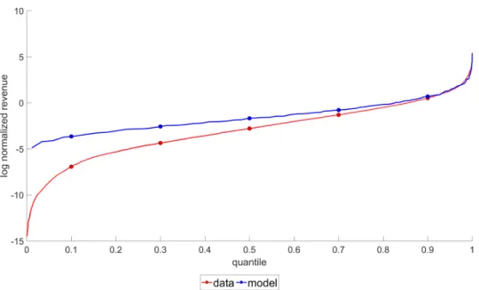
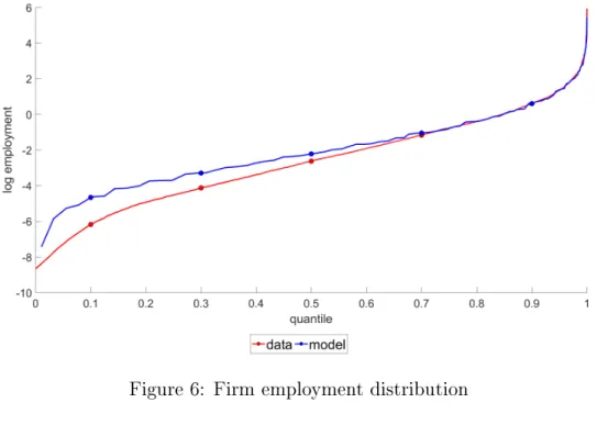
First, given that the empirical rm size distribution has a log-normal shape (see Figure 2 below), I assume that the log of fundamental rm productivities and demands, φ and δ, are also jointly Gaussian. Note that in the empty network with m χ, χ⁰

= 0 for all χ, χ⁰ ∈S_χ, this assumption would imply that rm revenue is exactly log-normally distributed.

Furthermore, one can easily verify that the model is invariant to jointly scaling the population size L, the mean relationship cost ψ, and the mean of rm fundamental characteristics. As such, the mean of the distribution of rm fundamental characteristics is normalized to zero.

In addition, I adopt a sparse parameterization of the model by assuming that φ and δ are uncorrelated, and that their marginal distributions share the same variance parameter v².

Parameterization of the xed relationship cost is as follows. First, I assume that the stochastic component of the cost shock ξt has a Weibull distribution with shape parameter s_ξ. The Weibull distribution has a simple economic interpretation as the minimum amongst a series of cost draws for a given relationship. The scale parameter of the distribution is then chosen so that the mean of ξ_t is equal to one.

4.3 Estimation procedure

With these parametric assumptions, the model developed in sections 2 and 3 has 8 pa- rameters: (1) the variance of fundamental rm characteristics,v²; (2) the mean relationship cost, ψ; (3) the shape of the relationship cost distribution, s_ξ; (4) the reset friction, ν; (5) the household discount factor, β; (6) the labor supply, L; (7) the elasticity of substitution, σ; and (8) the input suitability parameter, α.

I rst describe the set of parameters for which values are not estimated from data.

First, observe from either equation (3.12) or (3.14) that the parameters β and ν cannot be separately identied, as it is only the productβν that matters for the dynamic optimization problem of the rm. Since the Compustat data is of annual frequency, I therefore setβ =.95

and estimate ν from data. Second, since the model is scale invariant, the labor supply L is normalized to one. Third, since the Capital IQ and Compustat data do not contain trade transaction values from which substitution elasticities are typically estimated, I set the value of σ to 4, which is a typical value estimated in the literature.¹⁵

Finally, note that the input suitability parameter α can in principle be estimated from the available data, as it has an intuitive connection to a moment that can be empirically observed: when α is larger, more rm-to-rm relationships are likely to form. A potential indeterminacy arises, however, from the fact that a large number of active relationships can also be rationalized in the model by a low value of the mean relationship cost ψ. To avoid this indeterminacy in the estimation procedure, I therefore normalize α to a value arbitrarily close to but less than one, and rely on data to estimate the magnitude of the mean relationship cost instead. This approach can be interpreted as assuming that the cost of forming a relationship embodies not only the resources that need to be devoted to managing that relationship, but also the costs of technological innovation - design of prototypes and customization of products, for example - that are required for the seller's good to be used in the buyer's production process.

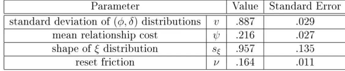
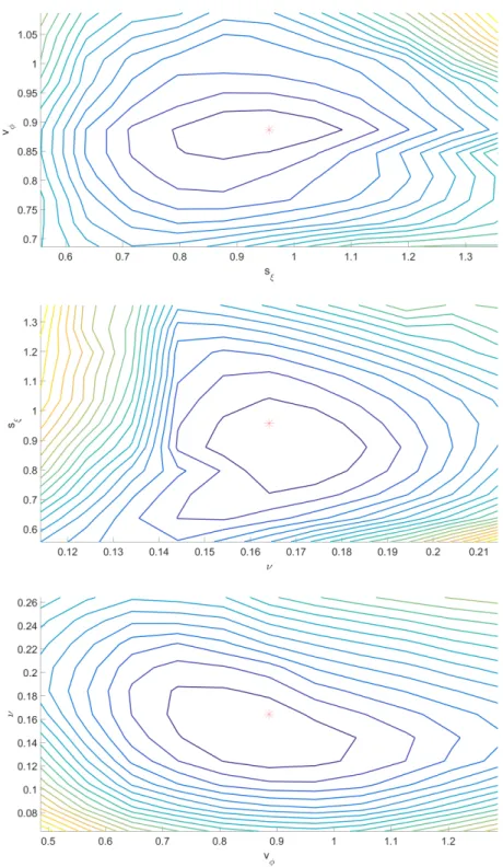
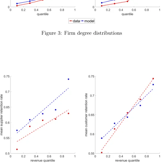
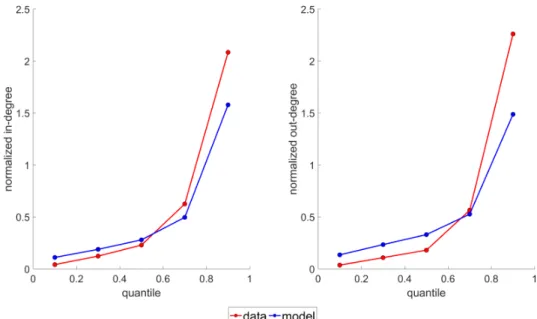
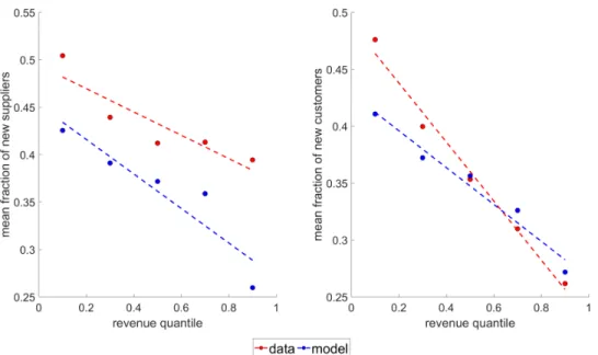
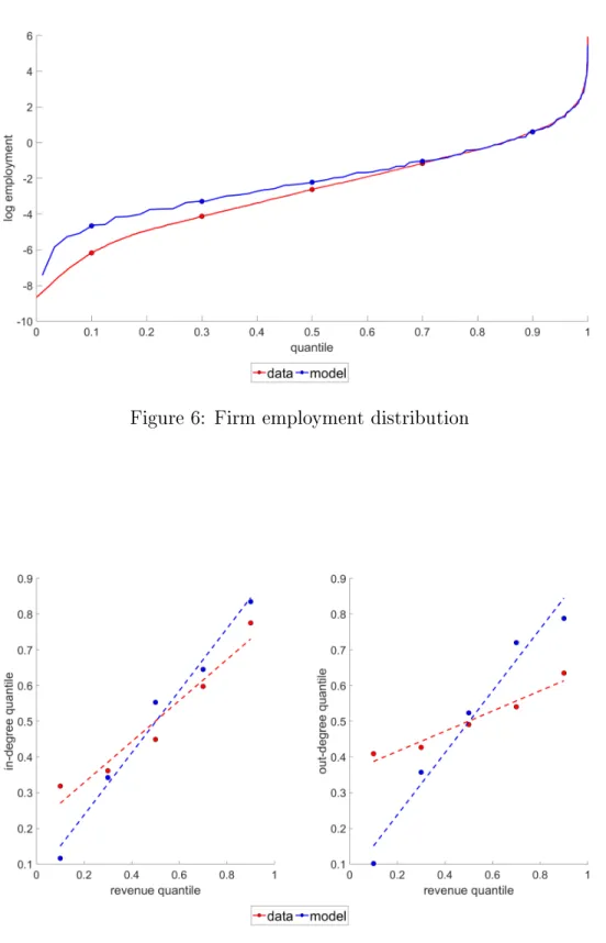
The remaining 4parameters of the model - v,ψ, s_ξ, andν - are then estimated from the Capital IQ and Compustat data using a simulated method of moments approach, targeting the following four sets of moments. First, the distribution of rm revenue normalized by its mean. Second, the distributions of in-degree (number of suppliers) and out-degree (number of customers). Third, the joint distributions of rm size and relationship retention rates (the fractions of suppliers and customers that are retained year-to-year). Fourth, the joint distri- bution of rm size and relationship creation rates (the fractions of suppliers and customers that are new year-to-year). The rst two sets of moments (static) are computed from the Capital IQ data, while the remaining two sets of moments (dynamic) are computed from the Compustat data.

Note that the dispersion of the rm and degree distributions are directly inuenced by the dispersion of rm fundamental characteristics v, while the dynamic moments are directly impacted by the volatility of the relationship cost shock s_ξ and the reset friction ν. These three parameters therefore have clear and intuitive connections to the data. The mean relationship costψ, which controls the overall level of connectivity in the production network, also has in principle a direct connection to the empirical average degree count. However, this is complicated by the fact that the degree count is continuous in the model but discrete in the data. To deal with this problem, I adopt a slight modication to the standard simulated method of moments approach in order to estimate ψ. Specically, given a set of values for

15See for example Broda and Weinstein (2006).