On the other hand, the irrational approach argues that addiction is a consequence of anomalies such as unexpected utility and hyperbolically discounted utility. The rational dependence model is compatible with traditional economic models such as discounted and expected utility schemes. Second, we investigate whether smokers who exhibit discounted and expected utility anomalies have higher rates of time preference and lower coefficients of risk aversion than nonsmokers who show evidence of the same anomalies.
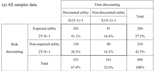
The standard theory of decision making under risk is the expected utility model advocated by Von Neumann and Morgenstern (1953). Looking at (a), which is the data from all samples, the incidence rate of the discounted utility anomaly is 32.6%, while that of the expected utility anomaly is 42.5%. Note that the incidence rate of homo economicus—satisfying both the discount and expected utility hypotheses—is 41.1%.
On the other hand, the incidence rate of non-homoeconomicus – which violates both the discounted and expected utility hypotheses – is 16.2%. Viewed from another point of view, the homoeconomicus ratios – satisfying both the discounted and expected utility hypotheses – are 37.2% for smokers and 45.2% for nonsmokers. The expected utility anomaly ratios are 44.1% for pachinko players and 42.0% for pachinko nonplayers.
Next, we explain the discounted and expected utility models that form the basis for estimating time preference rates and risk aversion coefficients.
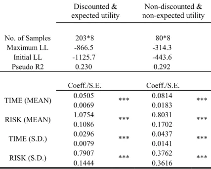
The Estimation Results of Conjoint Analysis
Conditional logit (CL) models, which assume independent and identical distribution (IID) of random terms, have been widely used in previous studies. However, the property of independence of the irrelevant alternatives (IIA), derived from the IID assumption in the CL model, is too strict to allow flexible substitution patterns. These models are flexible enough to overcome the limitations of CL models by allowing random flavor variation, unconstrained substitution patterns, and the correlation of random terms over time (McFadden and Train 2000).
In what follows, we assume that the time and risk preference parameters follow a normal distribution. We can demonstrate variation in the parameters at the individual level, using the maximum simulated likelihood (MSL) method for estimation, by setting 100 Halton draws9. Furthermore, with respondents answering eight questions in the conjoint analysis, the resulting data form a panel, giving us the option of applying standard random effects estimation.
We can now calculate the estimator of the conditional mean of the individual-level random parameters. The estimation results are presented in Table 2, separately, for the samples "both discounted and expected" (203), and for "both not discounted and. Since the volume of estimation results is large, we leave the estimates of others and we only show time preference rates and risk aversion coefficients below.
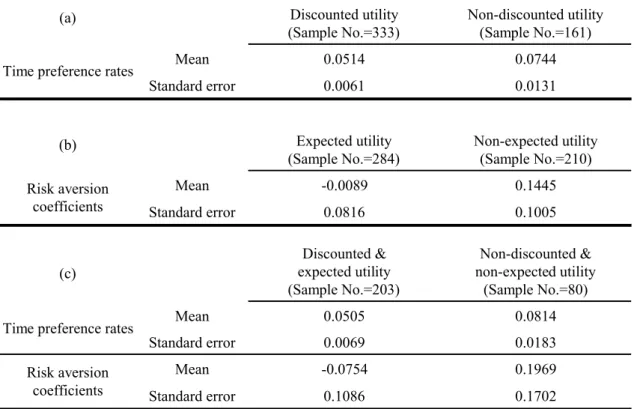
Based on the estimation results, we measured the time preference rates and the risk aversion coefficients for various cases. Furthermore, the results for the pachinko players and non-pachinko players are indicated in Tables 6 and 7.
Anomaly and Impulsivity for All Data
On the other hand, the interpretation of the latter result in relation to risk preference is difficult, because the expected utility anomaly is associated with risk-averse preferences and is not necessarily impulsive. This may explain the well-known fact that, contrary to expectations, smokers do not always discount risk more than non-smokers. Since the t-values are 14.69 for the time preference rates and 13.28 for the risk aversion coefficients, it can be claimed that the time and risk preferences differ significantly between the two types.
Finally, we can conclude that the discounted utility anomaly is associated with higher levels of time preferences, and the expected utility anomaly is associated with higher risk aversion coefficients.
Anomaly and Impulsivity for Smokers
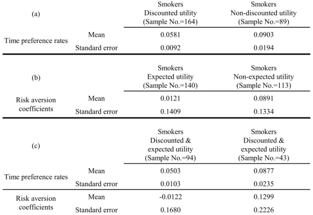
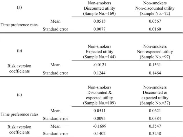
Following Ida and Goto (2009 in press), we simultaneously measured time preference rates and risk aversion coefficients. Here we are concerned with the following differences in rates of time preference: first, between discounted utility smokers and nonsmokers of the same type; and second, between non-discounted utility smokers and non-smokers of the same type. Similarly, we examine differences in risk aversion coefficients: first, between expected utility smokers and non-smokers of the same type, and second, between unexpected utility smokers and non-smokers of the same type. type.
The time preference percentages are 5.81% for the discounted utility smokers and 5.15% for the same type of non-smokers (see Tables 4(a) and 5(a)). Because the t-value is 7.06, the time preference rates are significantly different between smokers and nonsmokers within the discounted utility type. The time preference rates are 9.03% for the non-discounted utility smokers and 5.67% for the same type of non-smokers (see Tables 4(a) and 5(a)).
Because the t-value is 12.05, the time preference rates are significantly different between the non-discounted utility smokers and the non-smokers of the same type. Note that the difference between the utility smokers and non-smokers without a discount (Result 2.2) is larger than that between the utility smokers and non-smokers with a discount (Result 2.1). The risk aversion coefficients are 1.21% for the expected utility smokers and –1.21% for the same type of non-smokers (see Tables 4(b) and 5(b)).
Since the t-value is 1.53, the risk aversion coefficients are not significantly different between expected service smokers and non-smokers of the same type. The risk aversion coefficients are 8.91% for service unexpected smokers and 15.31% for the same type of non-smoker (see Tables 4(b) and 5(b)). Since the t-value is 3.29, the risk aversion coefficients are significantly different between utility service unexpected smokers and non-smokers of the same type.
These results for the risk aversion coefficients are only partially as expected; smokers are more risk averse than non-smokers only when the expected utility anomaly occurs (Result 2.4). To summarize these results, when the discounted and/or expected utility deviations occur, the time preference rates are higher and the risk aversion coefficients are lower for smokers than for non-smokers12. As such, the grounds for addiction are simultaneously provided by the weak rationality and the irrationality approaches.
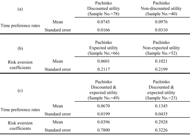
Anomaly and Impulsivity for Pachinko
The time preference rates are 9.76% for nondiscount utility pachinko players and 6.14% for non-players of the same type of pachinko (see Tables 6(a) and 7(a) ). Since the t-value is 7.18, the levels of time preferences are significantly different between non-discounted utility pachinko players and non-discounted utility pachinko players. First, we observed that the results obtained for smokers regarding time preference levels also hold for pachinko players.
The risk aversion coefficients are 6.01% for expected utility pachinko players and 0.10% for the same type of pachinko non-players (see Tables 6(b) and 7(b)). Since the t-value is 2.19, the risk aversion coefficients differ significantly between the expected utility pachinko players and non-players. The risk aversion coefficients are 10.21% for non-expected utility pachinko players and 12.20% for the same type of non-players (see Tables 7(b) and 7(b)).
Since the t-value is 0.63, the risk aversion coefficients are not significantly different between the non-expected utility pachinko players and non-players. In contrast to Finding 2.4 for smoking, Finding 3.4, regarding the risk aversion coefficients for the non-expected utility pachinko players and non-players, did not support the hypothesis. Although the exact background of this result remains unclear, it is at least certain that the complementarity between impulsivity and anomaly is less obvious for risk preference than for time preference.
The results obtained for pachinko (result 3.5) are more robust than those for smoking (result 2.5), and all expected results are reproduced for pachinko. Overall, time preference rates were higher among the undiscounted utility addicts, for activities such as smoking and gambling, than among the non-addicts of the same type.
Conclusion
Therefore, the ML choice probability is a weighted average of the logit probability Lnit(n) evaluated at parameter n with density function f(n), which can be written as. In linear parameter form, the utility function can be written as Unit 'xnit n'znit nit,. Unit *TIME*timedelaynit * ln probabilitynit*RISK* lnrewardnitnit, where is a scale parameter that is not identified separately from free parameters and is normalized to one (Hensher, Rose and Green 2005, p. 536)13.
Goto Interdependency among Addictive Behaviors and Time/Risk Preferences," Graduate School of Economics, Kyoto University, COE Simultaneous Measurement of Time and Risk Preferences:. Note: Coefficients in top row, standard error (S.E.) in bottom row, ** * at 1% significance level, ** at 5% significance level,.