PAPER
Global Nonlinear Optimization Based on Wave Function
and Wave Coefficient Equation
Hideki SATOH†, Member
SUMMARY A method was developed for deriving the ap-proximate global optimum of a nonlinear objective function with multiple local optimums. The objective function is expanded into a linear wave coefficient equation, so the problem of maxi-mizing the objective function is reduced to that of maximaxi-mizing a quadratic function with respect to the wave coefficients. Because a wave function expressed by the wave coefficients is used in the algorithm for maximizing the quadratic function, the algorithm is equivalent to a full search algorithm, i.e., one that searches in parallel for the global optimum in the whole domain of def-inition. Therefore, the global optimum is always derived. The method was evaluated for various objective functions, and com-puter simulation showed that a good approximation of the global optimum for each objective function can always be obtained.
key words: nonlinear, global optimization, wave function, quan-tum computing
1. Introduction
Conventional global optimization methods are classi-fied into random search methods and gradient meth-ods. The former randomly evaluate an objective func-tion to search for the global optimum. That is, they have to evaluate the objective function over the en-tire search space in principal. They thus need much computation time to find the global optimum; other-wise we cannot confirm whether the solution obtained is the global optimum. The latter use the derivative of an objective function to asymptotically search for the global optimum. The objective function thus must be differentiable, and the global optimum cannot always be derived although less computation time is needed.
One of the most serious problems in deriving the global optimum is avoiding falling into a local opti-mum because it is quite possible for all the methods expect the full search method to fall into a local op-timum. Tunneling algorithms [1], [2], [3] first search for a local optimum using a gradient method and then search for a better local optimum using a tunneling method starting from the local optimum previously ob-tained. The complex dynamics of a chaotic attractor is applied to various optimization methods to avoid being trapped in a local optimum [4]. Hopfield neu-ral networks (HNNs) [5] define an energy function de-rived from an objective function, and the state of the
Manuscript received June 11, 2009. Manuscript revised August 19, 2009.
†The author is with Future University Hakodate,
Hakodate-shi, 041-8655 Japan.
HNN changes in accordance with the energy function until the state becomes stable. A solution is then de-rived from the stable state. Boltzmann machines [6] are variations of HNNs to which a stochastic param-eter is added so that the state first changes stochas-tically, and the stochastic changes in the state gradu-ally decrease. With this parameter, the state falls into a local optimum less frequently. Simulated annealing (SA) [7] is a random search method that was devel-oped for performing random searches more effectively. It uses the principle of annealing from metal engineer-ing: slowly cooling heated metal produces a superior crystalline structure. Genetic algorithms (GAs) [8] are also random search methods; they use the principle of organic evolution to achieve the same thing. A solu-tion is considered to be an individual living creature, and it is improved by using mutation and combinations of information for various individuals. Although these methods have been well developed, they unfortunately cannot always derive the global optimum.
These methods are designed to avoid being trapped in a local optimum by using random variables, chaos, the structure of the objective function, or the relation-ship between local optimums. However, there is a fun-damental limit to their ability because they search for the global optimum in a real space. Quantum mechan-ics was recently added to some optimization methods to overcome this difficulty. Instead of SA thermal fluc-tuations in a real space, quantum annealing (QA) uses quantum fluctuations and thus has a shorter conver-gence time [9], [10]. Quantum neural networks (QNNs) [11], [12] are variations of HNNs and were developed to effectively perform a full search on the basis of the su-perposition of quantum states. Because QA and QNNs use the properties of a quantum mechanical system, they can find the global optimum without falling into a local optimum. However, it is very difficult to observe the quantum dynamics of a wave function and to con-struct a device to create the quantum effects that are required for QA and QNNs. It is thus still difficult to apply them to most optimization problems.
A method for global optimization has been devel-oped that overcomes the defects of the methods de-scribed above. A nonlinear objective function with multiple local optimums is expanded into a linear func-tion of a wave coefficient vector, and the problem of maximizing the objective function is reduced to that of
maximizing a quadratic objective function. Because it uses the wave function [13] expressed by the wave coef-ficients, it is equivalent to a full search method, i.e., one that searches in parallel for the global optimum in the whole domain of definition. Therefore, it can always find the approximate global optimum. The method is presented in this paper, and its validity is demonstrated using various objective functions. Computer simulation showed that it can always produce a good approxima-tion of the global optimum for each objective funcapproxima-tion if there is a unique global optimum.
2. Wave Coefficient Equation for Nonlinear Objective Function
A wave coefficient equation (WCE) was developed to reduce the problem of maximizing a nonlinear objec-tive function to that of maximizing a quadratic func-tion with respect to the wave coefficients. The moment vector equation (MVE) [14] of the objective function is first derived and is then transformed into the WCE. The MVE is summarized in Sect. 2.1, and the WCE for the objective function is presented in Sect. 2.2. 2.1 Moment Vector Equation
The MVE was developed to approximate an arbitrary multi-dimensional nonlinear function in the whole do-main of definition [14]. Consider the following nonlinear function:
y = f (x), (1)
where xdef= (x1, · · · , xdx)
T ∈ Dx is the state vector of
dimension dx, Dx def= {x|xmind< xd < xmaxd, 1 ≤ d ≤ dx} is the domain of the definition of x, y ∈ Dy is the value of f (x), Dy def= {y|ymin < y < ymax} is the
domain of the definition of y, and superscript T denotes transposition. If the domain of definitions cannot be set in advance, we can modify Eq. (1) to obtain
y = hy(f (hx(x))), (2)
where hy(y0) is a monotone increasing function such
that ymin≤ hy(y0) ≤ ymaxfor −∞ ≤ y0≤ ∞, hx(x)def=
(hx1(x1), · · · , hxdx(xdx))
T, and h
xd(xd) is a monotone
increasing function such that −∞ ≤ hxd(xd) ≤ ∞ for
xmind≤ xd≤ xmaxd.
Let {ψi(y)} and {ψi(x)} be orthonormal bases
de-fined in Appendix A. Note that the same symbol, ψ, is used to simplify the explanation, although {ψi(y)}
and {ψi(x)} are generally different bases. To derive
the MVE for the nonlinear function in Eq. (1), the fol-lowing assumption is introduced with respect to Eq. (1).
Assumption 1: We can expand E[ψi(y)|x] into a
Fourier series: E[ψi(y)|x] = Nx X j=0 aijψj(x) + εi(x), (3)
where Nx is the degree of expansion of E[ψi(y)], E[·] is
the mathematical expectation, and εi(x) is the residual.
2
Using Eq. (3), we can expand E[ψi(y)]:
E[ψi(y)] = Z ψi0p(ψi0)dψ0i = Z ψi0 Z p(x)p(ψ0i|x)dxdψ0i = Z p(x) Z ψ0ip(ψ0i|x)dψ0idx = Z p(x)E[ψ0 i|x]dx = Z p(x)( Nx X j=0 aijψj(x) + εi(x))dx = Nx X j=0 aijE[ψj(x)] + E[εi(x)], (4) where ψ0
i denotes ψi(y) and p(x) denotes the
proba-bility density function (pdf) of x. When Eq. (1) is deterministic, aij is obtained using Eq. (A· 2):
aij =
Z
Dx
ψi(f (x))ψ∗j(x)dx, (5)
where superscript ∗ denotes a complex conjugate. If we assume that E[εi(x)] = 0, Eq. (4) can be expressed
using a linear function:
E[ψ(y)] = AψE[ψ(x)]. (6)
This equation is referred to as the MVE, ψ(y) def= (ψ0(y), · · · , ψNy(y))
T, N
y is the degree of expansion of y, ψ(x)def= (ψ0(x), · · · , ψNx(x)) T, and Aψ def= a00 · · · a0Nx .. . . .. ... aNy0· · · aNyNx .
The nonlinear function in Eq. (1) is approximately expressed by the MVE in Eq. (6). The accuracy of Eq. (6) increases as Nxand Ny increase. Using Eq. (6), we
can derive not only the expected value of ψi(y) but also
the statistical properties such as the mean, variance, covariance, and pdf of y [14].
2.2 Wave Coefficient Equation
Let Ψ(x) be a wave function [13]. We can expand Ψ(x) using orthonormal basis {ψi(x)}:
Ψ(x) ∼= Nx X i=0 ciψi(x) = cTψ(x), (7)
where ci is the expansion coefficient of the wave
func-tion, which is referred to as the wave coefficient in this paper, and cdef= (c0, · · · , cNx)
T. As shown in Appendix
A, the wave coefficient can be obtained using
ci=
Z
Dx
Ψ(x)ψ∗
i(x)dx. (8)
Probability density function p(x) is obtained using Ψ(x) [13]:
p(x) = Ψ(x)Ψ∗(x)
∼
= ψT(x)cc†ψ∗(x), (9)
where superscript † denotes conjugate transposition. Because Rp(x)dx = RΨ(x)Ψ∗(x)dx = 1 and basis
{ψi(x)} is orthonormal, the following equation holds
[13]:
kck = 1,
where kckdef= √cTc∗.
Consider the pdfs defined by p(x)def= δ(x − ˆx) and p(y)def= δ(y − ˆy). Let ˆq be the wave coefficient vector
of p(x) and ˆr be that of p(y). Using Eq. (A· 9) in
Appendix B, we can obtain the wave coefficient vectors by using
ˆ
qdef= ξq−1ψ∗(ˆx), (10)
ˆ
rdef= ξr−1ψ∗(ˆy), (11)
where ξq and ξr are defined in the same manner as in
Eq. (A· 10). The normalization condition with respect to the wave coefficient is hereinafter eliminated. That is, kˆqk = 1 and kˆrk = 1 do not always hold†. From
Eq. (9), we obtain
p(x) ∼= kˆqk−2ψT(x)ˆqˆq†ψ∗(x), (12)
p(y) ∼= kˆrk−2ψT(y)ˆrˆr†ψ∗(y). (13)
We can modify Eq. (6) to obtain
ξr−1E[ψ∗(y)] = ξr−1ξqA∗ψξq−1E[ψ∗(x)].
Because p(x) = δ(x − ˆx) and p(y) = δ(y − ˆy), ψ∗(ˆx) = E[ψ∗(x)] and ψ∗(ˆy) = E[ψ∗(y)]. Thus, by substituting
Adef= ξr−1ξqA∗ψ and Eqs. (10) and (11) into the above
†Even if kˆqk = 1, kˆrk = 1 does not always hold in
Eq. (14) because matrix A is not a unitary matrix. Thus, the normalization conditions with respect to ˆq and ˆr were omitted.
equation, we obtain ˆ
r = Aˆq. (14)
This equation is an approximation of Eq. (1) based on the (unnormalized) wave coefficient vectors and yields
p(y) from p(x) assuming that p(x) and p(y) are delta
functions.
Let us generalize Eq. (14) for an arbitrary pdf. Consider the following equation for arbitrary wave co-efficient vectors q and r:
r = Aq. (15)
This equation is referred to as the wave coefficient equa-tion (WCE) in this paper. As shown in Appendix C,
p(x) is obtained from q, r is obtained from q as in Eq.
(15), p(y), which is related to p(x) by Eq. (1), is ob-tained from r, and matrix A in Eq. (15) is obob-tained from Eq. (1). Thus, Eq. (14) can be generalized as Eq. (15), which expresses the nonlinear function in Eq. (1) for arbitrary q, and p(x) and p(y) are obtained using
p(x) ∼= kqk−2ψT(x)qq†ψ∗(x), (16)
p(y) ∼= krk−2ψT(y)rr†ψ∗(y). (17)
3. Global Optimization in Wave Coefficient Space
A global optimization method based on the WCE in Eq. (15) is presented in this section.
Consider the optimization problem of maximizing
y ∈ Dy obtained by Eq. (1) for x ∈ Dx. Using WCE
in Eq. (15) and pdf in Eq. (17), we can rewrite the op-timization problem as the problem of maximizing E[y] defined by E[y] def= Z yp(y)dy = Z
ykrk−2rTψ(y)ψ†(y)r∗dy
= kAqk−2qTATY A∗q∗, (18)
where Y def= Ryψ(y)ψ†(y)dy is an (N
y+ 1) × (Ny+ 1)
matrix (See Appendix D for details). If kAqk2 = qTATA∗q∗ = 1, Eq. (18) reduces to qTATY A∗q∗.
Thus, the optimization problem of maximizing E[y] is expressed as
Object : max
q qTATY A∗q∗, (19)
Constraint :qTATA∗q∗= 1. (20)
Because the objective function of this problem is a quadratic equation with respect to q, we can solve
the above optimization problem using the steepest de-scent method (SDM) in a wave coefficient space for the following Lagrange function [17]:
L(q, µ)def= −qTATY A∗q∗+ µ(qTATA∗q∗− 1),(21)
where µ(−∞ ≤ µ ≤ ∞) is the Lagrange multiplier. The algorithm is described in Algorithm 1.
Algorithm 1: Steepest descent method in a wave co-efficient space for Lagrange function L(q, µ).
(1-1) Set t = 0.
(1-2) Set step sizes αq, αµ, and αstep (all > 0) and
initial values q0 and µ0. (1-3) Compute dqt and dµt: dqt= −∇Re[q]L(qt, µt) − ı∇Im[q]L(qt, µt), dµt= −∇µL(qt, µt). (1-4) Compute qt+1and µt+1: qt+1= qt+ αqdqt, µt+1= µt− αµdµt.
(1-5) If R(t, αstep) = 0 and Jopt(t)−Jopt(t−αstep) < 0,
set ˜qopt= qt and finish the algorithm.
(1-6) Set t = t + 1 and go to Step (1-2).
Here, R(t, αstep) is the remainder of t upon division by αstep, Jopt(t)def= E[y]t/(
P
dσ[xd]t), αstepis set to a
nat-ural number to eliminate small fluctuations in Jopt(t), ∇x denotes the nabla operator with respect to x, E[y]t
is defined using Eq. (18) as
E[y]tdef= kAqtk−2qtTATY A∗q∗t, (22)
and σ[xd]tis defined as σ[xd]tdef= q E[xd2]t− E[xd1]2t, (23) E[xdn]t = Z xdnp(x)dx ∼ = Z xdnkqtk−2qtTψ(x)ψ†(x)q∗tdx = kqtk−2qtTXd(n)q∗t, (24) Xd(n)def= Z xdnψ(x)ψ†(x)dx. (25)
The reason the condition for finishing the algorithm in Step (1-5) is used will be discussed in Sect. 4.2.
The approximation of the global optimum,
E[xd]opt, which approximately maximizes Eq. (1), and
the approximate maximum of Eq. (1), E[y]opt, are
ex-pressed using ˜qopt obtained using Algorithm 1:
E[xd]opt = k˜qoptk−2q˜optTXd(1)˜q∗opt, (26)
E[y]opt def= kA˜qoptk−2q˜optTATY A∗q˜∗opt. (27) The calculation cost of Algorithm 1 is not lower than that of conventional methods because Algorithm 1 is based on the steepest decent method. Although we can reduce its calculation cost using the property of the objective function in Eq. (19), which is a convex quadratic function, it is very difficult to obtain higher performance with respect to the calculation cost com-pared with conventional methods, which have been im-proved over a long period of time through various ap-plications. Two properties of Algorithm 1, the global optimum is always obtained (as shown in Sect. 4) and Algorithm 1 uses a wave function, are more important than the calculation cost because they are also proper-ties of quantum computing [15].
That is, the solution described in Eqs. (26) and (27) is obtained using the wave coefficient vector, which describes a quantum state. This is the same as in quan-tum computing. However, there are differences between the method presented in this paper and quantum com-puting.
• Quantum mechanics describes a linear relationship in quantum states.
• Quantum computing transforms input quantum state c to output quantum state c0 using unitary operator U . Thus, kck = kc0k always holds. • In contrast, the WCE in Eq. (15) describes a
non-linear objective function in Eq. (1), so matrix A is not unitary. That is, krk = kqk does not always hold.
• This means that the WCE in Eq. (15) expresses a nonlinear relationship in real space by omitting the restriction of unitary representations from matrix A.
It is thus difficult to apply the WCE to quantum com-puting directly. The application of the method pre-sented in this paper to quantum computing is left for future work.
4. Performance Evaluation
Algorithm 1 presented in this paper reduces the opti-mization problem for a nonlinear objective function in Eq. (1) to that for a convex quadratic objective function with a convex quadratic equality constraint in Eqs. (19) and (20). Generally, we cannot always derive a global optimum for both functions. However, Algorithm 1 uses a wave function expressed in a wave coefficient space and a distribution of global optima for Eq. (1) can be expressed by a pdf with a wave coefficient vector regardless of the number of global optima. Algorithm 1 is thus equivalent to a full search algorithm if its ini-tial state expresses a uniform distribution. Therefore, a global optimum should always be obtained. In this section, Algorithm 1 is examined for various objective functions to evaluate its performance.
Table 1 Parameters of fG(x1) used to examine condition for finishing Algorithm 1. ` 1 2 3 4 5 β` 0.50 0.85 0.50 0.70 0.60 γ1` 0.08 0.20 0.35 0.55 0.80 ζ1` 0.05 0.05 0.05 0.15 0.10 4.1 Objective Functions
Consider the problems of maximizing Gaussian-type function fG(x) and square-type function fS(x), defined
by fG(x)def= α + NXextrm `=1 β` dx Y d=1 exp(−(xd− γd`) 2 ζ2 d` ), (28) fS(x)def= α + NXextrm `=1 β` dx Y d=1 squ(xd, γd`, ζd`), (29)
where each fG(x) and fS(x) is the superposition of
functions with a unique extreme, Nextrm is the
num-ber of the superposition, α is the minimum value of
fG(x) and fS(x), β` is the weight of the `th extreme
value, γd` is the coordinate of the `th extreme value on
the xd-axis, ζd` is the width of the `th extreme value,
and squ(xd, γd`, ζd`) is a one-dimensional square
func-tion defined by squ(xd, γd`, ζd`)def= ( 1 if γd`− ζd` 2 <xd≤γd`+ ζd` 2 0 otherwise.
4.2 Condition for Finishing Algorithm 1
Consider one-dimensional Gaussian-type function fG(x1)
with Nextrm = 5, dx = 1, α = 0.05, 0 ≤ x1 ≤ 1.0,
0 ≤ y ≤ 1.0, and the parameters in Table 1. As we can see from Table 1 and the objective function shown in Fig. 1, there are four local optimums, and the global op-timum, x1opt, is equal to 0.2 (= γ12). Using Algorithm
1 with Nx = Ny = 128, we can derive the global
opti-mum. Here, αq = 10−3, αµ = 10−3, and αstep = 104.
Figure 2 shows the changes in E[y]t and E[x1]t, which
are defined by Eqs. (22) and (24), respectively. Figures 3 and 4 show the changes in pt(x) and pt(y), respec-tively, which are the pdfs at the tth step defined by
pt(x)def= kqtk−2ψT(x)qtqt†ψ∗(x), (30)
pt(y)def= kAqtk−2ψT(x)Aqtqt†A†ψ∗(x). (31)
The q0 and µ0 values are initialized: q0 =
(1, 0, · · · , 0)T and µ
0 = 0. The former means that p0(x1) is a uniform distribution. Here, after the
con-dition for finishing the algorithm is satisfied, the al-gorithm is continued until t = 108 to investigate the
Fig. 1 fG(x1) defined in Table 1
.
Fig. 2 Changes in E[x1]tand E[y]tobtained using Algorithm
1 for fG(x1) in Fig. 1.
convergence process.
As shown in Fig. 2, E[x1]tchanges from E[x1]0=
0.5, which is the mean value of the uniform distribu-tion, toward the global optimum (x1opt= γ12) passing
through the local optimum (γ13), and reaches the global
optimum at about t = 104. We can see in Fig. 3 the
change in pt(x1); Algorithm 1 takes the whole value of x1 into account in accordance with pt(x1) at each step
rather than investigates fG(x1) for various values of x1
step by step.
Once E[x1]tconverges to global optimum x1opt at
about t = 104, it separates from x
1opt, as shown in Fig.
2. Because Eqs. (19) and (20) are quadratic forms, it is clear that there are many values of q that satisfy Eqs. (19) and (20). However all values of q do not necessar-ily satisfy kqk = 1 because matrix A is not a unitary matrix. Algorithm 1 thus can select various values of q as a solution even if they do not satisfy kqk = 1. This means that the solution may not express the correct pdf of x1. This behavior of Algorithm 1 can be
con-firmed by comparingFigs. 2 through 5. The shape of
Fig. 3 Change in pt(x1) obtained using Algorithm 1 for fG(x1)
in Fig. 1.
correct pdf of x1when the optimal value is obtained, at
about t = 104, as shown in Fig. 3. As shown in Fig. 5, kqtk and kAqtk once converge to almost 1 at the same
time. However, kqtk separates from 1 whereas kAqtk
remains near 1. The reason for this latter behavior is that Eq. (20) works as a constraint in Algorithm 1, and the reason for the former behavior is that matrix A is not a unitary matrix. The value of E[x1]t separates
from x1opt, as shown in Fig. 2, and the shape of pt(x1)
collapses as kqtk separates from 1, as shown in Fig. 3.
However, E[y]ttakes the maximum value even though
kqtk separates from 1, as shown in Fig. 2. It is thus
clear that these changes in E[x1]tand pt(x1) arise from
the change in kqtk and that there are many values of qtthat maximize E[y]teven though it does not express
an appropriate pdf. Figure 4 shows that pt(y) retains the delta function while E[y]t takes a maximum value even though pt(x1) is separate from the delta function.
This means that the optimization problem for y can be replaced with that for E[y], as described in Appendix D.
As mentioned above, E[x1]tobtained by Algorithm
1 does not always express the optimal value even if E[y]t
takes the maximum value. We can find whether qt
obtained by Algorithm 1 expresses an appropriate pdf by using the sum of the differences between the norm and 1, defined by |kqtk − 1| + |kAqtk − 1|. It becomes
almost zero, as shown in Fig. 5, if the pdf is appropriate.
Fig. 4 Change in pt(y) obtained using Algorithm 1 for fG(x1)
in Fig. 1.
Fig. 5 Change in norm of wave coefficient vector obtained us-ing Algorithm 1 for fG(x1) in Fig. 1.
However, it cannot be used as the condition for deciding whether E[x1]tis optimum because E[x1]tis not always
optimum when it is equal to zero.
To investigate the condition for finishing the algo-rithm immediately after E[x1]tconverges to x1opt, the
changes in E[y]t, σ[x1]t, and E[y]t/σ[x1]t were
evalu-ated, as shown in Fig. 6. Algorithm 1 maximizes E[y]t,
and E[y]t remains maximum after E[x1]t is separated
from the global optimum. In this sense, Algorithm 1 works well. However, we can see in Figs. 3 and 6 that various shapes of pt(x) yield the maximum value. That
Fig. 6 Changes in E[y]t, σ[x1]t, and E[y]t/σ[x1]tobtained
us-ing Algorithm 1 for fG(x1) in Fig. 1.
Fig. 7 Effect of Nxon accuracy of solution for fG(x1) in Fig.
1.
is, there are many solutions of q that maximize E[y]t.
Therefore, the value of E[y]t should not be used as
the condition for finishing Algorithm 1. In contrast,
E[y]t/σ[x1]t is almost maximum and σ[x1]t is almost
minimum when E[x1]t ∼= x1opt. Because various
eval-uations (the results are omitted in this paper) showed that E[y]t/σ[x1]t is superior to σ[x1]t from the
view-point of solution accuracy, E[y]t/σ[x1]t is used as the
condition for finishing Algorithm 1 (Step (1-5) in Algo-rithm 1).
4.3 Evaluation
The effect of Nx on the accuracy of the solution was
evaluated for one-dimensional Gaussian-type function
fG(x), which is the same function used in Sect. 4.2. Here, Ny is set equal to Nx. As shown in Fig. 7, good
approximations of the global optimum were obtained when Nx≥ 16, and the accuracy of the approximations
increased with the value of Nx.
Consider two-dimensional Gaussian-type function
Table 2 Corresponding table for functions, parameter table, and figures of functions and ˜popt(x).
Function Parameter table Function p˜opt(x)
fG(x)|uniGO Table 3 Fig. 8 Fig. 9
fS(x)|uniRGO Table 3 Fig. 10 Fig. 11
fG(x)|twoGO Table 4 Fig. 12 Fig. 13
Table 3 Parameters for fG(x) with unique global optimum
and fS(x) with unique region of global optimum.
` 1 2 3 4 β` 0.60 0.85 0.40 0.20 γ1` 0.20 0.80 0.20 0.80 ζ1` 0.20 0.20 0.20 0.20 γ2` 0.20 0.20 0.80 0.80 ζ2` 0.20 0.20 0.20 0.20
Table 4 Parameters for fG(x) with two global optimums.
` 1 2 3 4 β` 0.60 0.85 0.85 0.20 γ1` 0.20 0.80 0.20 0.80 ζ1` 0.20 0.20 0.20 0.20 γ2` 0.20 0.20 0.80 0.80 ζ2` 0.20 0.20 0.20 0.20
Fig. 8 fG(x)|uniGOdefined in Table 2.
fG(x) and two-dimensional square-type function fS(x)
with Nextrm = 4, dx = 2, α = 0.05, 0 ≤ x1 ≤ 1.0,
0 ≤ x2 ≤ 1.0, 0 ≤ y ≤ 1.0, and the parameters in
Table 3 or 4. The relationship between the function, the parameter table, the figure of the function, and the figure of ˜popt(x) defined by
˜
popt(x)def= k˜qoptk−2ψT(x)˜q
optq˜opt†ψ∗(x) (32)
is shown in Table 2, where fG(x)|uniGO denotes fG(x)
with a unique global optimum, fS(x)|uniRGO denotes fS(x) with a unique region in which ∀x are global opti-mums, and fG(x)|twoGOdenotes fG(x) with two global
optimums.
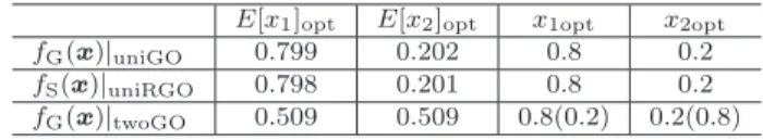
Table 5 shows the approximations of the global optimums for the three functions in Table 2. As shown in Table 5, the approximation of the global optimum for fG(x)|uniGO obtained using Algorithm 1
Fig. 9 p˜opt(x) for fG(x)|uniGOobtained using Algorithm 1.
Fig. 10 fS(x)|uniRGOdefined in Table 2.
Fig. 11 p˜opt(x) for fS(x)|uniRGOobtained using Algorithm 1.
to the global optimum (xoptdef= (x1opt, x2opt)T). In Fig.
9, we can see that ˜popt(x) is also a good approximation of δ(x − xopt). This result is consistent with the
re-sult in Sect. 4.2 because the fG(x)|uniGOshown in Fig.
8 is a differentiable function and has a unique global optimum in the same manner as the function in Sect. 4.2.
In contrast, fS(x)|uniRGOshown in Fig. 10 contains
regions where a derivative cannot be derived. More-over, the derivative in the regions where the function is differentiable is equal to zero. Therefore, it is not possi-ble to apply gradient methods to fS(x)|uniRGObecause
they use a derivative of the objective function. On the
Fig. 12 fG(x)|twoGOdefined in Table 2.
Fig. 13 p˜opt(x) for fG(x)|twoGOobtained using Algorithm 1.
other hand, many global optimums are obtained using random search methods. Thus, a somewhat compli-cated operation has to be added if it is necessary to eval-uate the relationship of the global optimums and to find the value representing them. In contrast, Algorithm 1 provides, without any additional operation, a solution that is the center of the global optimums to represent them. In Table 5, xopt and E[x]opt for fS(x)|uniRGO
denote the center of the global optimums and its ap-proximation obtained using Algorithm 1, respectively. We can see from Table 5 that Algorithm 1 provides a solution that represents the global optimums. The dis-tribution of the global optimums is obtained using their higher-order statistics such as standard deviation and
nth moment defined by Eqs. (23) and (24).
As shown in Fig. 12 and Table 5, fG(x)|twoGO has
two global optimums. Although an approximation of the pdf that expresses the global optimums was ob-tained, as shown in Fig. 13, the approximation of the global optimum in Table 5 is wrong because it is as-sumed in Eq. (26) that there is a unique global opti-mum. Deriving good approximations of the global op-timums from the pdf in Fig. 13 is a subject for future study.
As in the case of fG(x)|twoGO, a correct
approxi-mation of the global optimum is not always obtained. It is thus necessary to judge whether the approxima-tions of the global optimums in Table 5 are good or
Table 5 Global optimums and their approximations obtained using Algorithm 1.
E[x1]opt E[x2]opt x1opt x2opt
fG(x)|uniGO 0.799 0.202 0.8 0.2
fS(x)|uniRGO 0.798 0.201 0.8 0.2
fG(x)|twoGO 0.509 0.509 0.8(0.2) 0.2(0.8)
Table 6 Approximately maximum values of objective func-tions obtained using Algorithm 1.
E[y]opt f (E[x]opt)
fG(x)|uniGO 0.881 0.900
fS(x)|uniRGO 0.885 0.900
fG(x)|twoGO 0.886 0.077
not without having any knowledge useful for deriv-ing the global optimum. This can be done by com-paring E[y]opt with f (E[x]opt). As shown in Table 6, E[y]opt is almost equal to f (E[x]opt) when the
approx-imation of the global optimum is good (fG(x)|uniGO
and fS(x)|uniRGO). On the other hand, E[y]opt is far
from f (E[x]opt) when the approximation of the global
optimum is bad (fG(x)|twoGO). Therefore, we can
con-clude that we can derive a good approximation of the global optimum if there is a unique global optimum and that we can judge whether the approximation is good or bad.
5. Conclusion
A method was developed for deriving the global opti-mum of a nonlinear objective function with multiple lo-cal optimums. The objective function is expanded into a linear wave coefficient equation, and the problem of maximizing the objective function is reduced to that of maximizing a quadratic function with respect to the wave coefficients. The method was examined by com-puter simulation for various objective functions. It was shown that a good approximation of the global opti-mum of each objective function can always be obtained if the objective function has a unique global optimum and that the accuracy of the approximation increases with the degree of expansion of the nonlinear objective function. Although the calculation cost of the method is not lower than that of conventional methods, the method is based on a novel idea. Since it uses the wave function of the objective function, it should be possible to extend it into a quantum computing algorithm.
References
[1] A. V. Levy and A. Montalvo, “The tunneling algorithm for the global minimization of functions,” SIAM J. Sci. Statist. Comput., vol. 6, no. 1, pp. 15–29, 1985.
[2] P. Liu and B. J. Berne, “Quantum path minimization: an efficient method for global optimization,” Journal of Chem-ical Physics, vol. 118, no. 7, pp. 2999–3005, Feb. 2003.
[3] Wenzel W. Hamacher K, “Stochastic tunneling approach for globalminimization of complex potential energy land-scapes,” Physical Review Letters, vol. 82, no. 15, pp. 3003–
3007, April 1999.
[4] H. Nozawa, “A neural network model as a globally coupled map and applications based on chaos,” Chaos, vol. 2, no. 3, pp. 377–386, 1992.
[5] J. J. Hopfield and D. W. Tank, “Neural computation of de-cisions in optimization problems,” Biological Cybernetics, vol. 52, pp. 141-152, 1985.
[6] D. H. Ackley, G. E. Hinton, and T. J. Sejnowski, “A learn-ing algorithm for Boltzmann machines,” Cognitive Science, vol. 9, pp. 147-169, 1985.
[7] S. Kirkpatrick, C. D. Gelatt Jr., and M. P. Vecchi, “Op-timization by simulated annealing,” Science, vol. 220, no. 4598, pp. 671–680, May 1983.
[8] I. Ono and S. Kobayashi, “A real-coded genetic algorithm for function optimization using unimodal normal distribu-tion crossover,” Proc. 7th Int. Conf. on Genetic Algorithms, pp. 246–253, 1997.
[9] G. E. Santoro and E. Tosatti, “Optimization using quan-tum mechanics: quanquan-tum annealing through adiabatic evo-lution,” J. Phys A: Math. Gen., vol. 39, no. 36, pp. R393-R431, Sept. 2006.
[10] S. Morita and H. Nishimori, “Convergence theorems for quantum annealing,” J. Phys. A: Math. Gen., vol. 39, pp. 13903–13920, 2006.
[11] H. Nishimori and Y. Nonomura, “Quantum effects in neural networks,” Journal of the Physical Society of Japan, vol. 65, no. 12, pp. 3780-3796, 1996.
[12] M. Akazawa and E. Tokuda and N. Asahi and Y. Amemiya, “Quantum Hopfield network using single-electron circuits-a novel Hopfield network free from the local-minimum diffi-culty,” Analog Integrated Circuits and Signal Processing, vol. 24, no. 1, pp. 51–57, June 2000.
[13] S. Gasiorowicz, Quantum Physics 2nd Ed., John Wiley & Sons Inc., USA, 1996.
[14] H. Satoh, “Approximation and analysis of nonlinear equa-tions in a moment vector space,” IEICE Tans. Fundamen-tals, vol. E89-A, no. 1, pp. 270–279, Jan. 2006.
[15] M. A. Nielsen and I. L. Chuang, Quantum Computation and Quantum Information, Cambridge University Press, UK, 2000.
[16] I. N. Bronshtein and K. A. Semendyayev, Handbook of Mathematics, Springer-Verlag, UK, 1997.
[17] D. G. Luenberger, Linear and Nonlinear Programming, Addison-Wesley Publishing Company, USA, 1984.
[18] A. Papoulis, The Fourier Integral and its Applications, McGraw-Hill, USA, 1962.
Appendix A: Basis for Function Approxima-tion
An orthonormal basis is summarized in this ap-pendix. Let h(k) be the Fourier coefficient, k def= (k1, · · · , kdx)
T ∈ Z be the index vector of the Fourier
coefficient, and Z be the set of k that are used for the index vectors. The Fourier series expansion for function
f (x) is defined by [16] f (x) = X k∈Z h(k)K(x, k), (A· 1) h(k)def= Z Dx f (x)K∗(x, k)dx, (A· 2)
where xdef= (x1, · · · , xdx)
Tis the state vector of
dimen-sion dx, Dxdef= {x|xmind≤ xd ≤ xmaxd, 1 ≤ d ≤ dx} is
the domain of the definition of x, superscript ∗ denotes a complex conjugate, {K(x, k)} is a multi-dimensional orthonormal basis, and K(x,k) is defined by
K(x, k)def=
dx
Y
d=1
Kd(xd, kd). (A· 3)
Here, {Kd(xd, kd)} is a one-dimensional orthonormal
basis.
Let {φi(·)} be a basis the element of which is
de-fined by
φi(x)def= K(x, k), (A· 4)
where i is the index of the basis. When Zd def=
{0, 1, · · · , Nd} and Z is given by the Cartesian product
as Z = Z1× Z2×, · · · , ×Zds, the relationship between k and i can be obtained using
i = dx X d=1 kd dx Y d0=d+1 (Nd0+ 1), (A· 5)
where Nd is the degree of expansion of xd. Let N be
the degree of expansion of x. When Eq. (A· 5) holds,
N is expressed by N = dx Y d=1 (Nd+ 1) − 1, (A· 6)
where the dimension of the feature space with the basis is N + 1. The relationship between i and k is referred to as the index table.
The element of the orthonormal basis based on the complex Fourier series is defined as [18]
Kd(xd, kd)def= r 1 Dxd for kd= 0 r 1 Dxd exp(−ı k d+1 2 ω0d(xd−xmind)) for kd=1, 3, · · · r 1 Dxd exp(ı k d 2 ω0d(xd−xmind)) for kd= 2, 4, · · ·
where ı denotes the imaginary unit, ω0d def= 2π/Dxd,
and Dxd def= xmaxd− xmind.
Appendix B: Wave Coefficient of Delta Func-tion
Delta function δ(x − ˆx) is defined by [13] δ(x − ˆx)def= lim a→0 dx Y d=1 1 a√πexp(− (xd− ˆxd)2 a2 ), (A· 7) where ˆxdef= (ˆx1, · · · , ˆxdx)
T is a constant vector.
Con-sider the pdf defined by p(x) def= δ(x − ˆx). Its wave
function is expressed by [13] Ψ(x, ˆx) = lim a→0 dx Y d=1 1 (a2π)1/4exp(− (xd− ˆxd)2 2a2 + ıκ0(xd− ˆxd)), (A· 8)
where κ0 is the angular wave number.
Let ˆc def= (ˆc0, · · · , ˆcNx)
T be the normalized wave
coefficient vector of Ψ(x, ˆx). Using Eq. (A· 2), we
ob-tain ˆci=
Z
Ψ(x, ˆx)ψ∗ i(x)dx.
Because Ψ(x, ˆx) in the above equation is independent
of i, there is an appropriate constant, ξ, and substitu-tion of Eq. (A· 8) into the above equasubstitu-tion yields
ˆci= ξ−1ψ∗i(ˆx). (A· 9)
Because ˆci is a normalized wave coefficient, the
follow-ing equation should hold:
Nx X i=0 ˆciˆc∗i = ξ−2 Nx X i=0 ψ∗ i(ˆx)ψi(ˆx) = ξ−2(N x+ 1) dx Y d=1 Dx−1d = 1. We thus obtain ξ =pNx+ 1 dx Y d=1 1 p Dxd . (A· 10)
Appendix C: Wave Coefficient Equation for Arbitrary Probability Density Function
Because the WCE in Eq. (14) was derived assuming that the pdfs of x and y are delta functions, it is not clear whether Eq. (14) holds for any wave coefficient vector. In this appendix, Eq. (14) is extended to a WCE for arbitrary wave coefficient vectors.
In the same manner as for Eq. (10) in Sect. 2.2, consider the following wave coefficient vector for ˆx` ∈
Dx: ˆ
q`
def
= ξq−1ψ∗(ˆx`), (A· 11)
where ` = 1, 2, · · · , L, ˆx` 6= ˆxm for ` 6= m, and ξq is
defined in the same manner as in Eq. (A· 10). Let p`(x)
be the pdf corresponding to ˆq`. Using Eq. (12), we can
express p`(x) as
Consider pdf p(x) defined by p(x)def= L X `=1 w`p`(x), (A· 13)
where w`∈ R and w`≥ 0. Consider ˆy` obtained using
Eq. (1) as ˆ
y`= f (ˆx`).
When p(x) is defined by Eq. (A· 13) and y is obtained by Eq. (1), the probability density function of y is ex-pressed as p(y) ∼= L X `=1 w`p`(y), (A· 14)
where p`(y) is defined by
p`(y)def= kˆr`k−2ψT(y)ˆr`rˆ`†ψ∗(y), (A· 15)
ˆ
r`def= ξr−1ψ∗(ˆy`), (A· 16)
in the same manner as for Eq. (13). This is clear be-cause p`(x) ∼= δ(x − ˆx`) and p`(y) ∼= δ(y − ˆy`).
When Eq. (A· 14) holds, Eq. (14) can be rewritten as
ˆ
r`= Aˆq`. (A· 17)
Consider wave coefficient vector q defined by
qdef= L X `=1 w0 `ˆq`. (A· 18)
We can express an arbitrary q by using a sufficiently large L, appropriate constants w0
` ∈ R, and an
appro-priate ˆq`. Consider wave coefficient vector r defined by rdef= L X `=1 w0`rˆ`. (A· 19)
By substituting Eqs. (A· 18) and (A· 19) into Eq. (A· 17), we obtain
r = Aq. (A· 20)
Let us define the relationship between w` and w0`
as
w`= k
X
m
wm0 qmk−2kw`0qˆ`k−2. (A· 21)
Consider wave functions Ψ(x) and Ψ(y) defined by Ψ(x)def= kqk−1ψT(x)q, (A· 22)
Ψ(y)def= krk−1ψT(y)r. (A· 23)
Because kˆr`k ∼= 1 when we set kˆq`k = 1, p(x) in Eq.
(A· 13) and p(y) in Eq. (A· 14) can be expressed as
p(x) ∼= kqk−2ψT(x)qq†ψ∗(x), (A· 24)
p(y) ∼= krk−2ψT(y)rr†ψ∗(y). (A· 25)
As described above, Eq. (A· 20) shows that we can de-rive r for an arbitrary q using matrix A, and Eqs. (A· 24) and (A· 25) show that p(x) and p(y) related to
p(x) by Eq. (1) can be obtained using q and r. Thus,
Eq. (A· 20) expresses the nonlinear function in Eq. (1) for an arbitrary wave coefficient vector.
Appendix D: Optimization in Wave
Coeffi-cient Space
The relationship between the optimization problem for y and that for E[y] is described here. First, we clar-ify the meaning of maximizing E[y]. Let ymax be the
maximum value of y = f (x), and recall that
(1) E[y] is defined as E[y]def= Ryp(y)dy, as in Eq. (18). (2) The definitions of A, q, and Y and Eqs. (15) and (17) mean that an arbitrary p(y) including δ(y − ymax) can be obtained by modifying q.
From the above definitions, maximizing E[y] denotes adjusting q so as to maximize E[y].
Next, recall that ymax is equal to E[y] if p(y) =
δ(y − ymax). This means that we can obtain E[y] such
that ymax is equal to E[y] by adjusting the shape of
p(y). Because we can obtain an arbitrary shape of p(y) by adjusting q, it is possible to make E[y] equal ymax
by adjusting q.
In contrast, if max E[y] = ymax, p(y) = δ(y−ymax).
Because an arbitrary p(y) including δ(y − ymax) can
be obtained by modifying q, there exists q such that max E[y] = ymax. Therefore, we can replace the
opti-mization problem for y with that for E[y].
The change in p(y) is shown in Fig. 4, and we can confirm that p(y) = δ(y − ymax) when E[y] = ymax.
Note that the ˜popt(x) that provides ymax is not always
a delta function, as shown in Figs. 11 and 13, and that it was confirmed that they also provided p(y) = δ(y − ymax) although their figures were omitted in the paper.