重心系エネルギー7TeV での陽子・陽子衝突におけるボトムバリオン生成の研究

(1)

学位論文

Study of bottom baryon production in pp collisions

at

√

s = 7 TeV

（重心系エネルギー

7TeV

での陽子・陽子衝突における

ボトムバリオン生成の研究）

平成

27 年

12 月博士（理学）申請

東京大学大学院理学系研究科

物理学専攻

小森雄斗

(2)

Abstract

Studies of the production of the bottom baryons Ω−_b and Ξ−_b including their

antipar-ticles in pp collisions at √s = 7 TeV are performed using data corresponding to an

integrated luminosity of 4.5 fb−1 collected with the ATLAS detector at the LHC. The

bottom baryons are reconstructed in the decay modes of Ω−_b → J/ψ(→ µ+_µ−_)+Ω−₍_→

Λ0₍→ pπ−_)K−_{), Ξ}−

b → J/ψ(→ µ+µ−) + Ξ−(→ Λ0(→ pπ−)π−), and their charge con-jugates. A two-stage kinematical ﬁt is applied for reducing the background. A large number of the background are suppressed by the second ﬁt of imposing constraints

of the decay vertex positions and the masses of preselected J/ψ, Λ0_{, and Ω}− _(Ξ−₎

candidates in the first fit. After the kinematical selections on the finite lifetime and

the decay angle, the Ω−_b (Ξ−_b ) signals with 3.6σ (2.9σ) signiﬁcance were observed.

The masses were measured to be M_Ω−

b = 6035.8± 10.6(stat.)

+6.7

−1.1(syst.) MeV for the

Ω−_b baryon and M_Ξ−

b = 5775.9± 12.8(stat.)

+5.9

−0.8(syst.) MeV for the Ξ−b baryon. These

results are consistent with the measurements reported by the CDF and LHCb exper-iments. The production cross sections are also discussed.

(3)

-List of Figures

2.1 Baryon and meson models. . . 11

-2.2 JP _{= 0}− _{mesons. . . 12}

-2.3 JP = 1− mesons. . . 12

-2.4 Baryon octet. . . 13

-2.5 Baryon decuplet. . . 13

-2.6 Baryon octet extended to the bottom baryons. . . 14

-2.7 Baryon decuplet extended to the bottom baryons. . . 14

-2.8 Ω−_b mass distributions at the D0, CDF, and LHCb experiments [4] [10] [12]. . . 16

-3.1 Overall view of the LHC and its injectors [20]. . . 18

-3.2 Overall view of the LHC experiments [22]. . . 19

-3.3 Cutaway view of the ATLAS detector [23]. . . 20

-3.4 Geometry of the ATLAS magnet windings [23]. . . 21

-3.5 Cutaway view of the ATLAS inner detectors [23]. . . 23

-3.6 Cutaway view of the ATLAS calorimeter system [23]. . . 24

-3.7 3dimensional view of the ATLAS muon detectors [24]. . . 25

-3.8 Side view of the ATLAS muon detectors [24]. . . 26

-3.9 Block diagram of the ATLAS trigger system [25]. . . 27

-5.1 Image of the Ξ−_b and Ω−_b decay chains. . . 35

-5.2 pT (left) and η (right) distributions of the Ω−b (top) and Ξ−b (bottom) samples before the detector simulation. . . 37

-5.3 Muon reconstruction eﬃciency of the J/ψ trigger [33]. . . 38

-5.4 Integrated luminosity as a function of the day in 2011 [34]. . . 38

-5.5 Invariant mass distributions of the combined muon pairs. . . 40

-5.6 Invariant mass distributions of the combined muon pairs satisfying the quality requirements. . . 41

-5.7 Invariant mass distributions of the combined muon pairs in the data and the MC samples. . . 42

(7)

-LIST OF FIGURES LIST OF FIGURES

5.8 pT m, ηm, and ϕm distributions of the muons composing the J/ψ

can-didates. . . 42

-5.9 χ2 m, pT m, ηm, and ϕm distributions of the J/ψ candidates. Those pairs having χ2 m > 4 are included in the χ2m distribution. . . 43

-5.10 dR distributions between the truth J/ψ and the reconstructed J/ψ candidates. . . 44

5.11 J/ψ reconstruction eﬃciencies. . . 45

-5.12 Invariant mass distributions of the Λ0 _{candidates satisfying the quality} requirements. . . 47

-5.13 Illustration of Lxy for the Λ0 analysis. . . 48

-5.14 Lxy distribution of the Λ0 candidates. . . 49

-5.15 2-dimensional vertex position distribution of the Λ0 candidates in the sideband region. . . 49

-5.16 Invariant mass distributions of the Λ0 _{candidates satisfying all} requirements in the data and the MC samples. . . 50

-5.17 χ2 n, pT n, ηn, and ϕn distributions of the Λ0 candidates after the Lxy requirement in the signal region. . . 51

-5.18 dR distributions between the truth Λ0 and the reconstructed Λ0 can-didates. . . 52

-5.19 Λ0 _{reconstruction eﬃciencies.} _{. . . 53}

-5.20 Λ0 _{reconstruction eﬃciencies in L} xy at the truth level. . . 54

-5.21 Invariant mass distributions of the Ξ−candidates satisfying the quality requirements. . . 55

-5.22 Illustration of the pointing angle for the Ξ− analysis. . . 56

-5.23 Lxy distribution of the Ξ− candidates. . . 57

-5.24 cos θ distribution of the Ξ− candidates in the signal region. . . 57

-5.25 Invariant mass distributions of the Ξ−candidates satisfying all requirements in the data and the MC sample. . . 59

-5.26 χ2 n, pT n, ηn, and ϕn distributions of the Ξ− candidates in the signal region. . . 60

-5.27 2-dimensional invariant mass distribution for the Ξ− kinematics reﬂection. . . 61

-5.28 Invariant mass distributions of the Ω−candidates satisfying the quality requirements and removing the Ξ− kinematics reﬂection. . . 62

-5.29 Lxy distribution of the Ω− candidates. . . 63

-5.30 cos θ distribution of the Ω− candidates. . . 63

(8)

require-LIST OF FIGURES LIST OF FIGURES

5.32 χ2_n, pT n, ηn, and ϕn distributions of the Ω− candidates in the signal

region. . . 66

-5.33 pT 0, η0, and ϕ0 distributions of the proton and pion track parameters

used for the reﬁt for the data. . . 68

-5.34 pT 0, η0, and ϕ0 distributions of the proton and pion track parameters

used for the reﬁt for the MC sample. . . 69

-5.35 χ2_pm distributions of the Λ0 and Ω− candidates in the data and the MC

sample. . . 70

-5.36 pT pm, ηpm, and ϕpm distributions of the Λ0 and Ω− candidates after

the reﬁt for the data. . . 71

-5.37 Invariant mass distributions of the Ω−_b candidates in the data (right)

and the MC sample (left) satisfying the quality requirements. . . 72

-5.38 Illustration of the pointing angle and Lxy for the Ω−_b analysis. . . 73

-5.39 cos θ distributions of the Ω−_b candidates in the data and the MC sample. 74

-5.40 Lxy distributions of the Ω−b candidates in the data and the MC sample. 74

-5.41 Invariant mass distributions of the Ω−_b candidates satisfying the cos θ

and Lxy requirements. . . 75

-5.42 Deﬁnition of the decay angle. . . 76

-5.43 cos θ∗ distributions of the Ω−_b candidates in the data and the MC sample. 77

-5.44 Invariant mass distribution of the ﬁnal Ω−_b candidates in the data. . . 78

-5.45 Invariant mass distribution of the Ω−_b candidates in the MC sample

after applying all requirements. . . 78

-5.46 χ2

pm distributions of the Λ0 and Ξ−candidates in the data and the MC

sample. . . 79

-5.47 Invariant mass distributions of the Ξ−_b candidates satisfying the quality

requirements in the data (right) and the MC sample (left). . . 80

-5.48 cos θ distribution of the Ξ−_b candidates in the data and the MC sample. 80

-5.49 Lxy distribution of the Ξ−b candidates in the data and the MC sample. 81

-5.50 cos θ∗ distribution of the Ξ−_b candidates in the data and the MC sample. 81

-5.51 Invariant mass distributions of the Ξ−_b candidates satisfying the cos θ

and Lxy requirements. . . 82

-5.52 Invariant mass distribution of the Ξ−_b candidates satisfying all

require-ments in the data. . . 83

-5.53 Invariant mass distribution of the Ξ−_b candidates satisfying all

requirements in the MC sample. . . 83

-6.1 Invariant mass distributions of the Ω−_b (left) and Ξ−_b (right) candidates

(9)

-LIST OF FIGURES LIST OF FIGURES

6.2 Invariant mass distributions of the Ω−_b candidates with the ﬁt for the

data. . . 87

-6.3 Invariant mass distributions of the Ξ−_b candidates with the ﬁt for the data. . . 87

-6.4 The J/ψ, Ω−, and Ξ−mass distributions from the data (right) and the MC samples (left) with the ﬁtted curves. . . 90

-6.5 The Ω−_b masses at each experiment. . . 91

-6.6 The Ξ−_b masses at each experiment. . . 91

-6.7 Distribution of the mass diﬀerence for the Ξ∗−_b baryon [15]. . . 95

-6.8 Image of a double bottom baryon decay chain. . . 97

-A.1 Generated pT (left) and η (right) distributions of the Ω−b (top) and Ξ−b (bottom) samples. . . 101

-A.2 Invariant mass distributions of the Λ0 candidates satisfying the quality requirements in the MC samples. . . 102

-A.3 Lxy distributions of the Λ0 candidates in the MC samples. . . 102

-A.4 Invariant mass distributions of the Ω−(left) and Ξ− (right) candidates satisfying the quality requirements in the MC samples. . . 103

-A.5 Lxy distributions of the Ω−(left) and Ξ− (right) candidates in the MC samples. . . 103

-A.6 cos θ distributions of the Ω− (left) and Ξ− (right) candidates in the MC samples. . . 103

-A.7 dR distributions between the truth Ω−(left) and Ξ−(right) and the reconstructed Ω− and Ξ− candidates, respectively . . . 104

-A.8 Reconstruction eﬃciencies in Lxy of the Ω−(left) and Ξ−(right) candi-dates. . . 104

-A.9 Ω− and Ξ− reconstruction eﬃciencies. . . 105

-A.10 pT, η, and ϕ distributions of the Ω−b candidates in the data (right) and the MC sample (left). . . 106

-A.11 pT 0, η0, and ϕ0 distributions after the refit for the Ξ−b candidates (data). 107 -A.12 pT 0, η0, and ϕ0 distributions after the refit for the Ξ−b candidates (MC). 108 -A.13 pT pm, ηpm, and ϕpm distributions of the Λ0 and Ξ− candidates after the refit. . . 109

-A.14 pT, η, and ϕ distributions of the Ξ−b candidates in the data (right) and the MC sample (left). . . 110

-C.1 Invariant mass distributions of the Ω−_b (left) and Ξ−_b (right) candidates with the single Gaussian ﬁt in the MC samples. . . 112

(10)

-D.2 Ξ−_b signiﬁcance in cos θ∗. . . 114

-D.3 Invariant mass distributions of the Ω−_b (top) and Ξ−_b (bottom)

candi-dates with the shifted tracks. . . 115

D.4 µ distributions of the data and the MC sample. . . 116 D.5 Eﬃciencies in the average µ values. . . 116

(11)

-Chapter 1

Introduction

One of the most successful theory of the twentieth century in elementary particle physics is the Standard Model. In nature, there are four interactions: the weak, electromagnetic, strong, and gravitational interactions, and the Standard Model is able to describe the three interactions except for the gravitational interaction. The

four interactions are transmitted by three types of gauge bosons; the W± and Z

bosons for the weak interaction, photons for the electromagnetic interaction, and the gluons for the strong interaction. The weak and electromagnetic interactions are

based on and uniﬁed in the gauge theory of the group SU(2)× U(1) and the strong

interaction is described by that of the gauge group SU(3). The existence of these gauge bosons has been proved by various experiments.

When local gauge invariance is required, all particles need to be massless. To avoid this mathematical property, the spontaneous symmetry breaking of a scalar field is introduced. The scalar field is termed the Higgs field and emerges as a massive particle. This massive particle is the Higgs boson. The Higgs boson had not been observed for a long period, but it was finally discovered with the LHC at CERN in 2012, and the Standard Model strengthens its validity.

A basic theory of hadron physics is described by quantum chromodynamics (QCD) of the strong interaction in the framework of the Standard Model. Hadrons are considered to be bound states of quarks. Therefore, in principle, their properties such as their masses should be determined by QCD. This is, however, not yet a case for light hadrons composed of light quarks (u, d, s) because the eﬀective coupling of the theory increases as the energy scale determined by the hadron masses decreases. On the other hand, properties of heavy hadrons containing one or more heavy quarks (c, b) are better calculable since the perturbative approach is applicable because of

(12)

Baryons which include charm quarks are called charmed baryons, and also baryons with bottom quarks are bottom baryons. So far, six out of the sixteen bottom baryon ground-states with one bottom quark have been discovered [3] [4]. Most of them have been observed in the high energy hadron colliders of Tevatron and the LHC. Any double bottom baryons or bottom baryons with charm quarks have not been discovered yet.

Bottom baryons are new particles and their parameters are not measured suﬃ-ciently. Indeed QCD of the Standard Model is successful to describe hadron physics, but it still is not enough to evaluate the quality and integrity in the area of heavy hadrons. Therefore, understanding bottom baryons is an essential component in

QCD. Furthermore, it plays an important role of accurately estimating H0 → b¯b and

other exotic new physics with bottom quarks as bottom hadron production is to be backgrounds for the analyses [5].

In this thesis, bottom baryon production is studied using data taken with the LHC during the entire year of 2011. The theoretical background about bottom baryons is described in the next chapter. Chapter 3 describes the LHC and the ATLAS experiment. In Chapter 4, the method of calculating vertices is described. The

reconstruction strategy of the bottom baryons Ω−_b and Ξ−_b is detailed in Chapter 5.

The results of the mass measurements and the production cross sections are described in Chapter 6. Finally, in Chapter 7, the conclusions are described.

(13)

Chapter 2 Theoretical background

2.1 Hadron physics

Quark Anti-quark Baryon Meson

Figure 2.1: Baryon and meson models.

Hadrons are regarded as bound states of some quarks and/or anti-quarks by the strong interaction. Hadrons composed of three quarks are called ‘baryons’ and hadrons composed of one quark and one anti-quark are called ‘mesons’. Figure 2.1 shows a cartoon of a baryon and a meson.

The baryon number of one quark is deﬁned as 1₃. The number of baryons is 1 and

that of mesons is 0. The baryon number is generally conserved during known decays of standard hadrons.

2.1.1 Meson model

A quark spin (s) is 1₂. Therefore, a grand-state meson spin with zero orbital angular

momentum is 1 or 0; s = 1 in the case where the directions of the two quarks are the same, and s = 0 in the case where those are opposite. The parity operator of mesons is written as

(14)

2.1.2 Baryon model 2.1 Hadron physics

Here, a relationship of quarks parity is used (Pq=−P¯q). l means the orbital angular

momentum quantum number. In the light quark system, u-quarks, d-quarks, and

s-quarks are constituent particles of mesons and nine combinations of the two exist.

They are nine pseudoscalar mesons (J (≡ l + s)P _{= 0}−_{) and nine vector mesons}

(JP _{= 1}−_).

Q

Y

u¯

s

u ¯

d

¯

ds

¯

us

d¯

u

d¯

s

K

+

π

+

¯

K

0

π

−

K

0

π

0

η

′

1 -1

K

− Figure 2.2: JP = 0− mesons.

Q

Y

u¯

s

u ¯

d

¯

ds

¯

us

d¯

u

d¯

s

K

∗−

1 -1

K

∗+

ρ

+

¯

K

∗0

ρ

−

K

∗0

ρ

0

ω

φ

Figure 2.3: JP = 1− mesons.

Figures 2.2 and 2.3 show two types of the nine mesons. x-axis means a charge of the mesons and y-axis means a hypercharge of them. The hypercharge Y is deﬁned as summation of the baryon number B and the strangeness number S, i.e. Y = B + S. The strangeness number is the number of anti-s-quarks. The baryon number of mesons is 0, so that y-axis of the ﬁgures is identical to the strangeness number. The

π0 and ρ0 mesons at Q = Y = 0 are mixing states of the quark pairs u¯u and d ¯d. The

η, η′, and ω mesons are those of u¯u, d ¯d, and s¯s. The ϕ meson is almost a state of the

pure pair s¯s. The s¯s state of the ω meson has lesser impact on its state, therefore,

the ω state is written as ω ≃

√

1

2(u¯u + d ¯d).

2.1.2 Baryon model

Baryons are composed of three quarks. Therefore, the total angular momentum J

of a grand-state baryon with zero orbital angular momentum is 1₂ or 3₂. The total

wave function must be antisymmetric because of the Pauli exclusion principle as a quark is a fermion. A quark has a color from QCD and all hadrons are colorless. The following color wave function is permitted for baryons:

ψcolor =

1

√

(15)

2.2 Bottom baryon model Here, the part ‘RGB’ means that the ﬁrst quark color is Red, the second is Green, and the third is Blue. Equation (2.2) is antisymmetric under interchanges of the constituent quarks, so that the baryon wave function without the color part should be symmetric under the interchanges. These baryons, which are composed of u,

d, and s-quarks, belong to the ﬂavor symmetry group SU(3). The fundamental representation is classiﬁed as

3⊗ 3 ⊗ 3 = 1 ⊕ 8 ⊕ 8 ⊕ 10, (2.3)

and eighteen combinations among the twenty seven are allowed; the eight baryons

with J = 1₂ and the ten baryons with J = 3₂. The decuplet is totally symmetric

in the interchange of the quarks and therefore the J = 3₂ baryons satisfy the Pauli

exclusion principle. One of the octet baryons has a mixed symmetry, but it forms the

symmetric wave function by combining the mixed spin states of the J = 1₂ baryons.

In the end, these baryons are shown in Figures 2.4 and 2.5. The baryons Λ0 _{and Σ}0

at Q = Y = 0 in Figure 2.4 are the mixing states of the quark trios sud and sdu.

Q Y 1 -1 1 -1 udd uud uss uus dss sdd n p Σ+ Ξ0 Ξ− Σ− Σ0 _Λ0

Figure 2.4: Baryon octet.

Q Y 1 -1 1 -1 uud uus dss sdd 2 -2 ∆0 _∆+ _∆++ Σ∗+ Ξ∗0 Ω− Ξ∗− Σ∗− Σ∗0 ∆− udd uuu ddd uss sss uds

Figure 2.5: Baryon decuplet.

2.2 Bottom baryon model

Bottom baryons that contain one or more bottom quarks but no charm quark can be classiﬁed by the SU(4) group analysis similarly to the SU(3) representation of light baryons. The fundamental representation is a quadruplet that is composed of u, d,

(16)

2.2 Bottom baryon model Considering the Pauli exclusion principle like the previous section, twelve new baryons with bottom quarks should exist in addition to the basic baryon octet and new ten ones should exist in addition to the decuplet. Figures 2.6 and 2.7 show an extended version of Figures 2.4 and 2.5 including the bottom baryons. The bottom surfaces correspond to the octet and the decuplet of Figures 2.4 and 2.5, and z-axis (upper direction) shows the number of bottom quarks.

ssb usb uub udb dsb ddb sbb dbb ubb Σ+ p Σ− b Ξ− b _Ω− b Ξ0 b Σ+ b Λ0 b, Σ0b Ξ− bb Ω− bb Ξ0 bb dds uus uud uds uss Σ Ξ− Ξ0 Λ0 , Σ0 dss n udd

Figure 2.6: Baryon octet extended to the bottom baryons.

Ω− Ξ∗− Σ∗− ∆− ∆0 ∆+ Σ∗− b Ξ∗− b Σ∗0 Ξ∗0 Σ∗+ ∆++ ddd dds dss sss uss uus uuu uds udd uud Ξ∗0 b Σ∗0 b Ω∗− b Σ∗+ b ddb dsb ssb usb uub udb Ξ∗− bb Ω∗− bb Ξ∗0 bb Ω− bbb dbb sbb ubb bbb

Figure 2.7: Baryon decuplet extended to the bottom baryons.

The J = 1₂ bottom baryons Λ0_b, Σ±_b, Ξ_b0, Ξ−_b, and Ω−_b and the J = 3₂ bottom

baryons Σ∗±_b , Ξ∗0_b , and Ξ∗−_b have been discovered so far. Excited states of the Λ0_b and

Ξ−_b baryons have also been discovered [13]. The ﬁrst reported one is the Λ0

b baryon,

which had been observed at the S¯ppS proton-antiproton collider at CERN in 1991

[6]. The searched decay mode was Λ0

b → J/ψ Λ. Since then, various experiments

have observed the Λ0

b baryon, and the mass and other parameters have been precisely

measured. After the discovery of the Λ0_b baryon, any other bottom baryon had not

been observed for sixteen years. However, in 2007, the Σ±_b and Σ∗±_b baryons were

discovered by the CDF experiment [7] and the Ξ−_b baryon was discovered by the D0

experiment [8]. The searched decay modes were Σ±,∗±_b → Λ0

bπ±and Ξ−b → J/ψΞ−. A

series of discoveries of these new bottom baryons was made possible by high energy

collisions of proton-antiproton provided by Tevatron [9]. In 2008, the Ω−_b baryon

through the decay mode of Ω−_b → J/ψ Ω− was discovered by the D0 experiment

[10], and in 2011, the Ξ0_b baryon was discovered by the CDF experiment through

(17)

2.2 Bottom baryon model observation years including the latest particles.

Table 2.1: Bottom baryons listing [13].

Particle Mass year

Λ0 b 5619.5± 0.4 MeV 1991 Σ+_b 5811.3± 1.9 MeV 2007 Σ−_b 5815.5± 1.8 MeV 2007 Σ∗+_b 5832.1± 1.9 MeV 2007 Σ∗−_b 5835.1± 1.9 MeV 2007 Ξ−_b 5794.9± 0.9 MeV 2007 Ω−_b 6048.8± 3.2 MeV 2008 Ξ0 b 5793.1± 2.5 MeV 2011 Ξ∗0_b 5945.0± 0.7 ± 0.3 ± 2.7 MeV [14] 2012 Ξ∗−_b 5955.33± 0.12 ± 0.06 ± 0.50 MeV [15] 2015

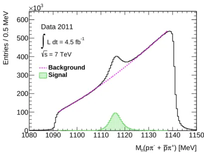
Although these bottom baryons are discovered, there are still a small number of candidates and the properties of the baryons are not yet known. For example,

the claimed mass of the Ω−_b baryon is diﬀerent between the measurements (CDF:

6054 MeV [12], D0: 6165 MeV [10]). Figure 2.8 shows the measured Ω−_b mass

dis-tributions from three experiments. The top left plot shows the result of D0, the top right plot shows that of CDF, and the bottom plot shows that of LHCb. Although the latest result from LHCb at the LHC supports the CDF result, new measure-ments are highly awaited for conﬁrmation. Especially, it is interesting to measure the production rate at the LHC energy.

(18)

) (GeV) b − Ω M( 5.8 6 6.2 6.4 6.6 6.8 7 Events/(0.04 GeV) 0 2 4 6 8 10 12 14 D0 −1 1.3 fb Data Fit (a) ] 2 c ) [MeV/ − Ω ψ M(J/ 5800 5900 6000 6100 6200 6300 ) 2_c Candidates / ( 20 MeV/ 0 2 4 6 8 10 12 14 16 18 20 22 24 LHCb − Ω ψ J/ → − b Ω (c)

Figure 2.8: Ω−_b mass distributions at the D0, CDF, and LHCb

(19)

Chapter 3 LHC and ATLAS experiment

3.1 Large Hadron Collider

The Large Hadron Collider (LHC) is the largest proton-proton collider in the world, having been built by the European Organization for Nuclear Research (CERN) lo-cated near Geneva in Switzerland. The purpose is to explore particle physics at the TeV scale; especially, to prove or disprove the existence of the Higgs boson, and it turned out that the Higgs boson does exist in 2012 [16] [17]. The mass is now determined to be 125.09 GeV by combining the ATLAS and CMS analyses [18].

The LHC is a circular accelerator. The design beam energy is 7TeV(√s = 14TeV)

and the design luminosity is 1034_cm−2_s−1_{. Here,} √_{s represents the total}

center-of-mass energy. To accomplish these performances, main 1232 superconducting dipole magnets cooled to 1.9 K by superﬂuid helium to provide a magnetic ﬁeld inten-sity of 8.33 T are arranged along the ring of 26.6 km in circumference [19]. Figure 3.1 shows an overall view of the LHC and its injectors. The proton beams from the linac are injected to the Proton Synchrotron (PS) via PS-booster to be accel-erated to 26 GeV. The beams are then sent to Super Proton Synchrotron (SPS)

and accelerated to 450 GeV. Finally, the beams are sent to the LHC ring,

ac-celerated, and stored for collisions. In November 2009, proton beams were circu-lated and the ﬁrst proton-proton collisions were recorded with the beam energy of

450 GeV (√s = 900 GeV). In March 2010, the highest-energy particle collisions with

the beam energy of 3.5 TeV (√s = 7 TeV) were recorded. Table 3.1 shows some values

(20)

3.1 Large Hadron Collider

Table 3.1: Details of the LHC parameters [21].

Design 2011

Circumferential length of the ring 27 km

-Proton beam energy 7 TeV 3.5 TeV

Peak luminosity/cm−2s−1 1034 3.65× 1033

The number of bunches 2808 1331

Time between bunch crossings 25 nsec 50 nsec

The number of proton particles per bunch 1.2× 1011 _1.2× 1011

(21)

3.2 ATLAS Detector

Figure 3.2: Overall view of the LHC experiments [22].

The LHC reuses a tunnel built for the Large Electron-Positron Collider (LEP, operated from 1989 to 2000) located about 100 m below ground. The LHC has four beam collision points, and four large detectors are placed at these collision points. Two of them are general-purpose particle physics detectors: ATLAS (A Toroidal LHC ApparatuS) and CMS (the Compact Muon Solenoid). The others are ALICE (A Large Ion Collider Experiment) and LHCb (Large Hadron Collider beauty). ALICE is a detector for heavy-ion (Pb-Pb) collisions, and LHCb aims for precise measurements of b-hadrons, especially on their CP violations. Figure 3.2 shows the locations of the four detectors.

3.2 ATLAS Detector

Figure 3.3 shows a cutaway view of the ATLAS detector. Its diameter is 25m, length is 44 m, and all-up weight is 7000 t. The inner track detectors, the calorimeters, and the muon track detectors are placed from the inside to the outside. The ATLAS detector is the largest detector in the world for collider physics and it is able to measure signals of electrons, muons, hadron jets, and missing transverse energy precisely under a severe high-luminosity condition.

(22)

3.2 ATLAS Detector

Figure 3.3: Cutaway view of the ATLAS detector [23].

interaction point to the center of the LHC ring and the y-axis points upward. A polar coordinate system is also frequently used, in which the polar angle θ is measured from the z-axis and the azimuthal angle ϕ is deﬁned as x = r sin ϕ and y = r cos ϕ with

r2 _{= x}2_{+ y}2_.

The rapidity y is deﬁned by the energy E and the longitudinal momentum p_∥ = pz

of a particle: y≡ 1 2ln ( E + p_∥ E− p_∥ ) = ln ( E + pz √ p2 T + m2 ) , (3.1)

where, m denotes the mass and pT is the transverse momentum (pT ≡

√

p2

x+ p2y). When the particle mass is negligible compared to the momentum, the pseudo-rapidity

η is often used instead of the rapidity. The pseudo-rapidity is deﬁned by the m→ 0

limit of the rapidity as

η = 1 2ln p + pz p− pz =− ln ( tanθ 2 ) . (3.2)

The barrel region of the detector covers an angular region of |η| < 1.05 and the

end-cap regions cover |η| > 1.05. The whole ATLAS detector covers a wide range of η up

(23)

3.2.1 Magnet systems 3.2 ATLAS Detector

3.2.1 Magnet systems

Figure 3.4: Geometry of the ATLAS magnet windings [23].

A large magnet system is incorporated in the ATLAS detector for precise measure-ments of charged particle momenta. Figure 3.4 shows a geometry of the ATLAS magnet windings. The ATLAS magnet system is composed of one solenoidal magnet located at the center of the detector and three sets of toroidal magnets around the calorimeters. All of them are superconducting magnets. The toroidal magnets are arranged to be an eight-fold azimuthal symmetry and generate an integrated mag-netic ﬁeld of 2 to 6 Tm at the barrel region and 4 to 8 Tm at the end-cap regions. The solenoidal magnet is arranged to cover the inner track detectors and generate an integrated magnetic ﬁeld of 2 T at the center. Using a curvature of charged particles by the magnetic forces, the momenta are measured.

3.2.2 Inner detectors

The inner detector are located in the magnetic ﬁeld produced by the solenoid magnet. Figure 3.5 shows a cutaway view of the inner detectors. They cover the pseudorapidity

range of |η| < 2.5. From the inside to the outside, pixel detectors, Semi-Conductor

Trackers (SCTs), and Transition Radiation Trackers (TRTs) are arranged. They measure the trajectories of charged particles in the magnetic ﬁeld to obtain their momentum information.

• Pixel detectors:

(24)

3.2.2 Inner detectors 3.2 ATLAS Detector detectors have a high resolution ability to measure the produced vertices of

charged particles. The size of one pixel is 50 µm × 300 µm in the z and ϕ

directions. The pixel detectors are placed very close to the interaction point, so that the occupancy is decreased by exploiting a beneﬁt of ‘pixelated’ detectors. The tracking resolution near the interaction point is 10 µm in rϕ and 115 µm along the z direction.

• SCT:

SCT is composed of long and thin microstrip silicon sensors arranged in par-allel rows. The distance between the strips is 80 µm. In each layer, the two sensors are paired and tilted with 40 mrad to allow a 2-dimensional position determination. The sensors are arranged in four cylindrical layers in the barrel region, and nine disks in each end-cap region. The position resolution is 17 µm in rϕ and 580 µm along z in the barrel region, and 17 µm in rϕ and 580 µm in

r in the end-cap region. • TRT:

TRT is composed of thirty-six layers of thin straw tube detectors covering a radius of 4 mm. TRT has the capability of identifying electrons by detecting X-rays of the transition radiations. TRT provides only rϕ information with the resolution of 130 µm.

(25)

3.2.3 Calorimeters 3.2 ATLAS Detector

Figure 3.5: Cutaway view of the ATLAS inner detectors [23].

3.2.3 Calorimeters

The energies of electrons, photons, and hadrons are measured with calorimeters. Figure 3.6 shows a cutaway view of the ATLAS calorimeter system. The

calorime-ters cover the pseudorapidity range of |η| < 4.9. They are located at the outside the

solenoid magnet and longitudinally divided into electromagnetic and hadron calorime-ters. The electromagnetic calorimeters measure energies and positions of electrons and photons. The hadron calorimeters surround the electromagnetic calorimeters and measure the energy of hadrons.

• Electromagnetic calorimeter:

The ATLAS electromagnetic calorimeter is composed of accordion-shaped lead absorbers and liquid argon as the active detection material. It has good

(26)

radi-3.2.4 Muon detectors 3.2 ATLAS Detector

Figure 3.6: Cutaway view of the ATLAS calorimeter system [23].

regions. The energy resolution is expressed as a function of the energy E [GeV] in the following formula,

∆σE

E =

9.5%

√

E ⊕ 0.7%, (3.3)

where ⊕ denotes the quadratic sum of the terms. The ﬁrst term comes from

statistical ﬂuctuation of shower tracks and the second constant term mainly comes from an accuracy of the calibration.

• Hadronic calorimeter:

Compositions of the hadron calorimeter are diﬀerent in each region. The barrel calorimeters are composed of iron absorbers and tiled plastic scintillators, while the end-cap calorimeters are composed of copper absorbers and liquid argon to preserve a good radiation resistance. The tungsten absorbers are also used in a foremost part of the end-cap regions, where higher energy particles are to be measured. The energy resolution is parameterized in the following formulae:

∆σE E = 52.3% √ E ⊕ 1.7% (Barrel), (3.4) ∆σE E = 62.4% √ E ⊕ 3.6% (End-Cap). (3.5)

3.2.4 Muon detectors

The muon lifetime is long and it seldom interacts with materials compared to other charged particles. Therefore, muons pass through the hadronic and electromagnetic

(27)

3.2.4 Muon detectors 3.2 ATLAS Detector chambers chambers chambers chambers Cathode strip Resistive plate Thin gap

Monitored drift tube

Figure 3.7: 3-dimensional view of the ATLAS muon detectors [24].

calorimeters of the ATLAS detector. The muon detectors are located outside all the other detectors to detect penetrated muons. Figures 3.7 and 3.8 show the ATLAS muon detectors. The muon detector system is composed of two types of detectors. One is used for generating trigger signals and the other is used for the position measurements. The former are Resistive Plate Chambers (RPCs) and Thin Gap Chambers (TGCs), and the latter are Monitored Drift Tubes (MDTs) and Cathode Strip Chambers (CSCs). RPCs are located in the barrel region and TGCs in the end-cap region. MDTs are placed in both barrel and end-end-cap regions with three stations to measure muon momenta. CSCs are located in a foremost part of the end-cap region to measure positions and angles of muons before entering into the end-cap

toroidal magnets. The muon detectors cover the pseudorapidity range of |η| < 2.7

for the momentum measurements and |η| < 2.4 for the triggers.

• RPC:

RPC is a parallel plate gas chamber without wires for the anode, in which

the C2H2F4 gas is ﬁlled between bakelite boards. The applied electric ﬁeld

between the boards is kept to a few kV/mm to produce spark-like signals in the passages of charged particles. The signals are read out from metal strips attached outside the bakelite boards. The strips in the two sides are arranged to be perpendicular to each other to provide a 2-dimensional measurement.

(28)

3.2.4 Muon detectors 3.2 ATLAS Detector 2 4 6 8 10 12 m 0 0 Radiation shield MDT chambers End-cap toroid

Barrel toroid coil

Thin gap chambers

Cathode strip chambers

Resistive plate chambers

14 16 18

20 12 10 8 6 4 2m

Figure 3.8: Side view of the ATLAS muon detectors [24].

• TGC:

TGC is a ‘Thin’ Multiwire Proportional Chamber (MWPC) ﬁlled with a mixed

gases of CO2 and n-Pentane. The applied electric ﬁeld is 3000 V. Tungstenic

wires with a radius of 25 µm are used as the anodes. The interval of the wire is 1.8 mm. Glass epoxy boards of carbons with the electrical resistance 1 MΩ are used as the cathodes. A 2-dimensional measurement is achieved by the readout of signals from the anode wires and metal strips attached outside the carbon cathodes. The position resolution is about 1 cm. Chambers composing TGC have a trapezoidal shape to cover the end-cap regions. The size of the chambers

ranges from 1 m× 1 m to 2 m × 2 m.

• MDT:

MDT is composed of six or eight layers of drift tubes with a radius of 15 mm. They are fastened on to a rigid frame. The ﬁlled gases is a composition of Ar

and CO2 under a pressure of 3 atm. An electric ﬁeld of 3270 V is applied to the

anode wire string at the center of each tube. The position resolution is 80 µm and the maximum drift time is 500 ns.

• CSC:

CSC is a cathodic readout MWPC. The distance between the wires is 2.5 mm and the distance between the strips is 5.3mm or 5.6mm. The position resolution is 60 µm and the maximum drift time is 30 ns. The ﬁlled gases is a composition

of Ar, CO2, and CF4 under a pressure of 3 atm with an anode voltage of 2600 V.

CSCs are located in a foremost part of the end-cap regions corresponding to

(29)

3.3 Trigger system which disturb the muon measurement.

3.3 Trigger system

LEVEL 2 TRIGGER LEVEL 1 TRIGGER

CALO MUON TRACKING

Event builder Pipeline memories Derandomizers Readout buffers (ROBs) EVENT FILTER Bunch crossing rate 40 MHz < 75(100) kHz O(1) kHz ~ 200 Hz Interaction rate ~1 GHz

Regions of Interest Readout drivers

(RODs)

Full-event buffers and

processor sub-farms

Data recording

Figure 3.9: Block diagram of the ATLAS trigger system [25].

On average, about twenty proton-proton collisions occur at each 40 MHz beam cross-ing in the design luminosity of the LHC. This corresponds to about 1 GHz proton-proton collisions. Therefore, it is important to select targeted physics events very eﬀectively. Figure 3.9 shows a block diagram of the ATLAS trigger system.

The trigger system is composed of three levels of triggers, and the trigger rate is reduced at each step. The steps are called as, ‘Level-1 trigger’, ‘Level-2 trigger’, and ‘Event Filter’. A task of the Level-1 trigger is to make a decision whether to start the readout or not, that of the Level-2 trigger is to make a decision whether to start an event building, and that of the Event Filter is to make decision whether to save the event.

(30)

by using the information from the muon detectors and the calorimeters, to

catch high-pT muons, electrons/photons, jets, or transverse missing momentum.

After receiving the trigger signals, triggered data of each event are collected on the Read Out Driver (ROD) and transferred to the Read Out Buﬀer (ROB). The location information of the trigger signal sources, which is called Region of Interest (RoI), is transferred to the Level-2 trigger. Here, the maximum trigger rate is reduced to 100 kHz.

• Level-2 trigger:

The Level-2 trigger is a software-base trigger performed in a computer form. The detector regions which should be examined are narrowed by using RoI transferred from the Level-1 trigger. Momenta and positons of the objects detected by the Level-1 trigger are recalculated in accordance with detailed information from the read-out data. At this stage, inner detectors information within RoI is available for reconstructing charged particle tracks. The decision of the Level-2 trigger is carried out using the result of the reconstruction. At this step, the trigger rate is reduced to a few kHz.

• Event Filter:

The event information which passed through the Level-2 trigger is transferred to the Event Filter after the event building. The Event Filter is also software-based. The decision of the Event Filter is carried out using the complete in-formation from the whole detectors. Contrary to the Level-2 trigger, only the information in RoI is available. Conclusions of the information from differ-ent detector compondiffer-ents are re-examined to iddiffer-entify interesting objects in each event. At this step, the trigger rate is finally reduced to about 200 Hz, to record the entire event data for effective analyses.

(31)

Chapter 4 Track parameters and vertex fit

Charged particle trajectories are reconstructed as helical tracks in the solenoidal magnetic field, to obtain their 3-dimensional momentum information. An appropriate assumption of the production vertex improves the reconstruction performance. For particles produced promptly, the production vertex is identical to the beam-beam collision point. However, such as assumption is not appropriate for decay products of long-lived particles that are considered in this analysis. The decay vertices, i.e., the production vertices of the decay products may be displaced from the collision point. The decay vertices are obtained from a simultaneous fit of the decay particle trajectories in the present study in order to optimize the momentum resolution for measured particles. Therefore, the vertex fit plays an important role in the analysis.

4.1 Track parameters

4.1.1 Parameterization of helical motion

The trajectory of charged particles in a magnetic ﬁeld can be obtained by solving an equation, ∂ ∂t ( mγ∂⃗r ∂t ) = kc2q⃗v(t)× ⃗B(⃗r), (4.1)

where ⃗B(⃗r) is the magnetic ﬁeld, ⃗r is a position of the particle, ⃗v is the particle

velocity, q is the signed charge, m is the rest mass, c is the velocity of light, t is the time, γ is the relativistic Lorentz factor, and k is the proportionality factor. In the

ATLAS inner detector, the magnetic ﬁeld ⃗B(⃗r) is almost parallel to the z-axis, so

(32)

4.1.2 Five track parameters 4.1 Track parameters of the above equation can be described as [26]

x(l) = x(0) + RH { cos ( Φ(0) + hl sin Θ RH ) − cos Φ(0) } , (4.2) y(l) = y(0) + RH { sin ( Φ(0) + hl sin Θ RH ) − sin Φ(0) } , (4.3) z(l) = z(0) + l cos Θ. (4.4) Here, Θ = sin−1 ( ∂z ∂l ) , RH = p sin Θ

|kqB| , and h = −sign(qBz). Equations (4.2), (4.3), and (4.4) denote the so-called parameterization of a helical motion in a global coor-dinate system. If the trajectory of a particle at the perigee is close enough to the origin, Equations (4.2), (4.3), and (4.4) can be written as the second order Taylor expansion around the perigee [26],

x ≃ −d0sin ϕ0+ (l sin θ0) cos ϕ0+

l2_sin2_θ 0

2hRH sin ϕ0, (4.5)

y ≃ d0cos ϕ0+ (l sin θ0) sin ϕ0 −

l2_sin2_θ 0

2hRH cos ϕ0, (4.6)

z ≃ z0+ l cos θ0, (4.7)

where variables denoted by the index 0 represent the values at the perigee and d0

represents the transverse impact parameter to the z-axis.

4.1.2 Five track parameters

Five track parameters are necessary to deﬁne a track as can be expected from the discussion in the previous subsection. The ﬁve variables are following:

• q

p: the charge over the momentum magnitude at the perigee.

• θ0: the polar angle at the perigee.

• ϕ0: the azimuthal angle at the perigee.

• z0: the z coordinate of the perigee.

• d0: the transverse impact parameter at the perigee.

These parameters are usually called the perigee parameters, and they can be

(33)

4.2 Vertex ﬁt

l0sin θ0 and RV ≡ yV cos ϕV − xV sin ϕV, the perigee parameters can be obtained as

the following functions:

ϕ0 = ϕV − L0 hRH . (4.8) z0 = zV − L0cot θ0. (4.9) d0 = RV + L2₀ 2hRH . (4.10)

Here, the variables denoted by the index V represent values at the origin V . Note

that q_p and θ0 do not change when going from V to the perigee.

4.2 Vertex ﬁt

4.2.1 Fit procedure

The ﬁve (5-dimensional) track parameters, qi described in the previous section and

their weight matrix Wi at the perigee obtained by individual track ﬁts are used for

the 3-dimensional vertex ﬁt. If a particle is originated from a vertex ⃗V , its track

parameters qi are able to be expressed as a function of the vertex position ⃗V and the

modiﬁed particle momentum ⃗pi at the vertex. To ﬁnd ⃗V and ⃗pi, minimization of the

following equation for χ2 is required:

χ2 = N∑tracks

i=1

(qi− T(⃗V , ⃗pi))TWi(qi− T(⃗V , ⃗pi)). (4.11)

Here, T(⃗V , ⃗pi) means trajectory parameters at a birthplace of the particle: q′i =

T(⃗V , ⃗pi). If T(⃗V , ⃗pi) is linearly related to the variations δ ⃗V and δ⃗pi around the ﬁrst

approximation ⃗V0 and ⃗p0i, T(⃗V , ⃗pi) can be written as follows:

T(⃗V , ⃗pi) = T(⃗V0+ δ ⃗V , ⃗p0i+ δ⃗pi) = T(⃗V0, ⃗p0i) + Diδ ⃗V + Eiδ⃗pi. (4.12) Here, Di ≡ ∂T(⃗V , ⃗pi) ∂ ⃗V and Ei ≡ ∂T(⃗V , ⃗pi) ∂⃗pi

are matrices of the derivatives. Then, Equation (4.12) can be written as

χ2 = N∑tracks

i=1

(34)

4.2.2 Fit constraint 4.2 Vertex ﬁt

where δqi = qi− T(⃗V0, ⃗p0i). To minimize Equation (4.13),

∂χ2

∂ ⃗V = 0 and

∂χ2 ∂⃗pi

= 0 are

required, and the system of equations for δ ⃗V and δ⃗pi are derived:

(_N tracks ∑ i=1 D_iTWiDi ) δ ⃗V + N∑tracks i=1 ( DT_i WiEi ) δ⃗pi = N∑tracks i=1 D_iTWiδqi, (4.14) ( E_iTWiDi ) δ ⃗Vi+ ( E_iTWiEi ) δ⃗pi = EiTWiδqi. (4.15)

Now, the vertex position ⃗V is equal to ⃗V0+ δ ⃗V and the modiﬁed particle momentum

⃗

pi equal to ⃗p0i+ δ⃗pi, so that a goal of the ﬁt is to solve the above equations and the

solution of δ ⃗V is [27] δ ⃗V = ( A− N∑tracks i=1 BiCi−1B T i )−1( F − N∑tracks i=1 BiCi−1Ui ) , (4.16) where A ≡ N∑tracks i=1 D_iTWiDi, Bi ≡ DTi WiEi, Ci ≡ EiTWiEi, F ≡ N∑tracks i=1 D_iTWiδqi, Ui ≡ EiTWiδqi.

δ⃗pi is able to be obtained by substituting δ ⃗V back into Equation (4.15).

If the ﬁrst approximation of ⃗V0 is far from the ﬁtted vertex, the track parameters

should be extrapolated to the ﬁtted point, all derivatives recalculated, and all ﬁt

procedures repeated. The weight matrices Wi should also be translated to the new

vertex position [28]. This method is completely the same as the Kalman ﬁlter based approach.

4.2.2 Fit constraint

The vertex ﬁt procedure without constraints is explained in Subsection 4.2.1. In this subsection, a vertex ﬁt procedure with constraints on some variables is explained.

It is beneﬁcial to impose some constraints in order to obtain more precise vertex positons and particle momenta. For example, when tracks are originating from well-known particles, a particle mass constraint is often imposed. The vertex ﬁt with

constraint Aj(⃗V , ⃗p1, ..., ⃗pn) = Const. is executed by using the Lagrange multipliers

method, i.e., using the following modiﬁed χ2 deﬁnition:

χ2 = χ2₀+∑ j

(35)

Here, χ2₀ is given by Equation (4.13), and λj denotes the Lagrange multiplier. If

A2

J can be linearized around the point (⃗V0, ⃗p0i) which is the solution without the

constraints (i.e. the case χ2 _{= χ}2

0), the above equation can be rewritten as

χ2 = χ2₀+∑ j λj(A2j0+ H T j δV + δV T_H j+ FijTδpi+ δpTi Fij), (4.18) where Hj = ∂Aj ∂ ⃗V , Fij = ∂Aj ∂⃗pi , Aj0 = Aj(⃗V0, ⃗p0i), δ ⃗V = ⃗V − ⃗V0, and δ⃗pi = ⃗pi− ⃗p0i.

To solve Equation (4.18), minimization of χ2 _{is carried out in the same way as the}

case without constrains by substituting ⃗V = ⃗V0+ ⃗V1 and ⃗pi = ⃗p0i+ ⃗p1i. The term ⃗V1

is the second part of the solution and can be obtained from the following relational expression [28]: ⃗ V1 =− ∑ j λjCcovLj, (4.19) where λj = Mj( ∑ i F_ijTC_i−1Fij + LTjCcovLj)−1, Lj = ∑ i BiCi−1Fij − Hj, Mj = A2j0− H T j V⃗0− ∑ i F_ijT⃗p0i, Ccov = (K − ∑ i BiCi−1B T i )−1, K =∑ i DT_i WiDi.

The deﬁnitions of the matrices Bi and Ci are the same as those in Subsection 4.2.1,

and ⃗p1i can be obtained in the same way. The vectors ⃗V0 and ⃗p0i are already solved

in the previous subsection, so that a goal of the ﬁt with constraints is accomplished as ⃗V = ⃗V0+ ⃗V1 and ⃗pi = ⃗p0i+ ⃗p1i.

In this analysis, the calculations of the vertex ﬁt are executed using a tool in the ATLAS software frame work [28]. The details of the actual application are described in the next chapter for the event reconstruction.

(36)

Chapter 5 Event reconstruction

5.1 Decay kinematics

The muon lifetime is long and it penetrates dense materials since it does not feel the strong force, i.e., the particle is clear enough to identify. In addition, the ATLAS detector has a good trigger eﬃciency on muons. Therefore, decay modes including muons in the ﬁnal state are suitable for studies of bottom baryons. The target decay modes in the present analysis are

Ω−_b → J/ψ + Ω−,

J/ψ → µ++ µ−, Ω− → Λ0+ K−,

Λ0 → p + π−,

for the Ω−_b baryon, and

Ξ−_b → J/ψ + Ξ−,

J/ψ → µ++ µ−, Ξ−→ Λ0+ π−,

Λ0 → p + π−.

for the Ξ−_b baryon. The ﬁve charged particles denoted by underlines are the objects

to be observed. The three particles other than the two muons can be distinguished by identifying the parent hadrons having a long lifetime. The vertex ﬁt described in Chapter 4 is used to identify these cascade decays. An image of these decays are

illustrated in Figure 5.1. The Ω−_b or Ξ−_b baryon is produced by a pp collision at the

collision point. The produced bottom baryon decays with a lifetime of O(ps) [3] to the

J/ψ meson and the Ω−/Ξ− baryon. The J/ψ meson immediately decays to a µ+_µ−

(37)

5.1 Decay kinematics

to the Λ0 baryon and the K−/π− meson with cτ = 2.461 cm/4.91 cm [3]. Here, the

K−/π− meson can be detected by the inner detectors. Finally, the Λ0 _{baryon decays}

to the proton and the pion with cτ = 7.89 cm [3] and they can also be observed by the inner detectors. Table 5.1 summarizes the masses and cτ values of the participating particles and Table 5.2 summarizes the relevant branching fractions.

π

−

p

K

−

/π

− Beam Beam Background

µ

−

µ

+

Λ

0

Ω

−

/Ξ

−

Ω

− b

/Ξ

−b

(38)

5.2 Monte-Carlo simulation Table 5.1: Masses and cτ values of the particles relevant to the analysis [3].

Particle Mass cτ /Lifetime(τ )

J/ψ 3096.916 MeV -Ξ− 1321.71 MeV 4.91 cm Ω− 1672.45 MeV 2.461 cm Λ0 _{1115.683 MeV} _{7.89 cm} µ± 105.658 MeV 658.6 m K− 493.677 MeV 3.7 m p 938.272 MeV τ > 1031_{to 10}33_yrs. π− 139.570 MeV 7.8 m

Table 5.2: Branching ratios of the particles relevant to the analysis [3].

Decay mode Fraction

J/ψ → µ+_µ− _5.93%

Ξ−→ Λ0π− 99.9%

Ω− → Λ0_K− _67.8%

Λ0 _{→ p π}− _63.9%

5.2 Monte-Carlo simulation

The properties of bottom baryons are still ambiguous because they have been discov-ered very recently. In order to understand the acceptance of the event selections, it is important to use a reasonable model of the bottom baryon production and to have the simulated event samples which are generated according to the model. pp colli-sion interactions are simulated using the Pythia event generator. Pythia simulates physics processes and the cross sections evaluated by using parton distribution func-tions of the initial state particles, matrix elements of parton-level hard interacfunc-tions, and fragmentations of produced partons.

In this analysis, generated events which include (anti-)Ω−_b or (anti-)Ξ−_b baryons

decaying to the ﬁnal states described in Section 5.1 are used. The bottom baryons

are selected through the fragmentation of b-quarks from gg → b¯b and q¯q → b¯b. They

have pT > 6 GeV in |η| < 2.7.

At least one of the two muons from the J/ψ decay has pT > 3.5 GeV in |η| < 2.5

(39)

5.2 Monte-Carlo simulation

0.13 for the Ω−_b simulation and 0.14 for the Ξ−_b simulation. The eﬃciency plots are

shown in Figure A.1 in Appendix A.1. The number of selected Ω−_b signal events is

366,998 and that of Ξ−_b events is 517,119.

In the simulations, the Ω−_b invariant mass is set to 6071.0 MeV, the world average

value in 2012 [3], and that of the Ξ−_b mass is set to 5791.1 MeV. The Ω−_b cτ is set to

0.339 mm and the Ξ−_b cτ is set to 0.447 mm.

The generated events are processed through the ATLAS detector simulation [30]

based on Geant4 [31]. Figure 5.2 show the pT and η distributions of the MC samples

before the detector simulation.

[MeV] T p b Ω MC truth 0 10000 20000 30000 40000 50000 Entries / 50 MeV 0 2000 4000 6000 8000 10000 12000 14000 16000 18000 20000 MC Simulation Sample -b Ω η b Ω MC truth -3 -2 -1 0 1 2 3 Entries / 0.1 0 2000 4000 6000 8000 10000 MC Simulation Sample -b Ω [MeV] T p b Ξ MC truth 0 10000 20000 30000 40000 50000 Entries / 50 MeV 0 5000 10000 15000 20000 25000 30000 MC Simulation Sample -b Ξ η b Ξ MC truth -3 -2 -1 0 1 2 3 Entries / 0.1 0 2000 4000 6000 8000 10000 12000 14000 MC Simulation Sample -b Ξ

Figure 5.2: pT (left) and η (right) distributions of the Ω−b (top) and

(40)

5.4 Muon track reconstruction

5.3 Data samples

The data used in the present analysis were collected in the year 2011 with a center-of-mass energy of 7 TeV of pp collisions. Those data were taken when the LHC beams were stable and all relevant detectors and magnets were running normally. Among the data, the events triggered by the J/ψ trigger are selected. The J/ψ trigger requires a detection of an opposite charge muon pair having an invariant mass within

the range of 2.5 < mµµ < 4.3 GeV [32]. The pT threshold of the muons is 4 GeV.

This trigger mode was prescaled in higher luminosity runs in 2012, whereas it was not prescaled during the 2011 data taking. As a reference, Figure 5.3 shows the muon reconstruction eﬃciency of the trigger at 7 TeV in 2010 evaluated on candidate

J/ψ→ µ+µ− events with respect to oﬄine muon reconstruction. The data eﬃciency

evaluated at plateau pT > 8 GeV is 0.41± 0.05 while the MC eﬃciency is 0.39 ± 0.04,

statistical errors only [33].

[GeV] T p 0 2 4 6 8 10 12 14 16 18 20 22 EF_2mu4_Jpsimumu Efficiency 0 0.1 0.2 0.3 0.4 0.5 0.6 0.7 0.8 0.9 ATLAS Preliminary -1 L dt = 38 pb ! 2010 Data MC Data |<2.4 " |

Figure 5.3: Muon reconstruction eﬃ-ciency of the J/ψ trigger [33]. Day in 2011 -1 fb T o ta l In te g ra te d L u m in o s it y 0 1 2 3 4 5 6 1/3 1/5 1/7 1/9 1/11 = 7 TeV s ATLAS LHC Delivered ATLAS Recorded -1 Total Delivered: 5.46 fb -1 Total Recorded: 5.08 fb

Figure 5.4: Integrated luminosity as a function of the day in 2011 [34].

The used data correspond to an integrated luminosity of 4.5 fb−1. Figure 5.4

shows the increase of the total integrated luminosity as a function of the day in 2011.

The integrated luminosity corresponding to the recorded data is 5.08 fb−1, and the

data committed by the J/ψ trigger are about 90% of them.

5.4 Muon track reconstruction

5.4.1 Muon reconstruction

Muons which pass the trigger system are reconstructed in the oﬄine software. They are classiﬁed into two types of muons: Stand Alone (SA) muons and ComBined (CB)

(41)

5.4.2 Muon selections 5.4 Muon track reconstruction muons. The SA muons are reconstructed by the Muon Spectrometer (MS) only. The CB muons, which are used in this analysis, are reconstructed by combining MS and ID track parameters. A combined ﬁt is performed using MS and ID track elements that make a nice accompaniment to each other in the (η, ϕ) plane by minimizing the

χ2 _{equation which is deﬁned as:}

χ2 = (P− PID)T× WID× (P − PID) + (P− PMS)T× WMS× (P − PMS), (5.1)

where PID and PMS are the two muon track parameters, WID and WMS are their

weight matrices, and P is the combined parameters to be optimized. The

opti-mization is tried for all candidate combinations, and the combination that gives the

smallest χ2 is retained. The optimized P of the best combination is taken as the

parameter of the combined muon track [25], and the combined muons with pT above

2.5 GeV are retained.

5.4.2 Muon selections

In order to obtain the final muon sample, the reconstructed muon tracks are regarded to be composed of a sufficient number of ID hits. This requirement is effective for reducing backgrounds from the pion and kaon in-flight decays and ensuring a good quality of the muon tracks. The requirements are [35]:

• nPixel ≥ 2:

nPixel is the number of hits in the pixel detector plus the number of dead pixel

sensors crossed by the track.

• nSCT ≥ 6:

nSCT is the number of hits in SCT plus the number of dead SCT sensors crossed

by the track.

• nHole

Pixel+ nHoleSCT < 3:

nHole

Pixel+ nHoleSCT is the number of missing hits in active layers of the pixel detector

and SCT.

• nb-layer ≥ 1:

nb-layeris the number of hits in the innermost layer (b-layer) of the pixel detector.

If the track is expected to pass outside the b-layer, this requirement is not applied.

(42)

5.5 J/ψ reconstruction

track reconstruction (nhits_TRT) plus that of TRT hits associated with the track but

not used (noutliers

TRT ), i.e., n = nhitsTRT+ noutliersTRT .

If |η| ≥ 1.9 and n ≤ 5, this requirement is not applied. If |η| ≥ 1.9 and n > 5,

noutliers

TRT < 0.9n is required.

If two opposite sign muons in an event satisfy the above requirements, the pair is used for the J/ψ reconstruction.

5.5 J/ψ reconstruction

Before starting the J/ψ vertex ﬁt, the invariant mass of the selected muon pairs

is required to be within the range of |M0(µ+µ−)− MPDG(J/ψ)| < 200 MeV. This

requirement reduces a lot of irrelevant combinations of muons. Here, the index 0 of M0

denotes the value calculated at the perigee. This requirement is loose enough to retain almost all J/ψ signals. The invariant mass distribution is shown in Figure 5.5 and the PDG average value is indicated as the red line. A partial sample corresponding to

the integrated luminosity of 11.6pb−1 is used for the plot. A clear peak corresponding

to the J/ψ signal can be seen, but the sample is still contaminated with background.

) [MeV] + µ -µ ( 0 M 2500 2600 2700 2800 2900 3000 3100 3200 3300 3400 3500 Entries / 2 MeV 0 200 400 600 800 1000 2011 Data -1 L dt = 11.6 pb

∫

TeV = 7 s Mass (3096.916 MeV) ψ J/

All CB muon pairs

Figure 5.5: Invariant mass distributions of the combined muon pairs.

Track parameters such as pT, η, and ϕ of the preselected muons are ﬁtted with

a constraint of the known J/ψ mass as described in Section 4.2. The ﬁt is carried out by assuming that the muon pair originates from a common vertex. Then, the following requirements are imposed to select a pure J/ψ sample. The requirements are

(43)

5.5 J/ψ reconstruction • χ2

m < 4,

• |ηm| < 2.5,

where the index m denotes a value after the ‘m’ass constraint. Figure 5.6 shows the invariant mass distributions evaluated by using the original track parameters of the muon pairs. The distributions are separately shown for the muon pair samples with

χ2_m > 4 or |ηm| > 2.5, and χ2m < 4 and |ηm| < 2.5. The χ2m > 4 or |ηm| > 2.5

pairs are rejected as the background. The obtained signal (χ2

m < 4 and |ηm| < 2.5) distribution is compared with simulation results in Figure 5.7. The left side plot

shows the comparison with the Ω−_b simulation and the right side one shows that with

the Ξ−_b simulation. The simulations are normalized to the number of entries. The

distributions are basically in good agreement with a small shift of the peak position.

The peak position is 3095.1 ± 0.2 MeV for the data, and 3101.1 ± 0.1 MeV and

3100.8±0.1MeV for the Ω−_b and Ξ−_b simulations, respectively. These mass diﬀerences

are used for estimating the systematic uncertainties in Subsection 6.1.4.

) [MeV] + µ -µ ( 0 M 2500 2600 2700 2800 2900 3000 3100 3200 3300 3400 3500 Entries / 2 MeV 0 200 400 600 800 1000 2011 Data -1 L dt = 11.6 pb

∫

TeV = 7 s > 4 m 2 χ Vertex | > 2.5 m η or | ) [MeV] + µ -µ ( 0 M 2500 2600 2700 2800 2900 3000 3100 3200 3300 3400 3500 Entries / 2 MeV 0 200 400 600 800 1000 2011 Data -1 L dt = 11.6 pb

∫

TeV = 7 s < 4 m 2 χ Vertex | < 2.5 m η |

Figure 5.6: Invariant mass distributions of the combined muon pairs satisfying the quality requirements.

Figure 5.8 shows the pT m, ηm, and ϕm distributions of the muons composing the

selected J/ψ candidates. There is no signiﬁcant bias depending on the sign of the charge. The eﬀective threshold of the selected muons is approximately 4 GeV due

to the trigger. The dips at |ηm| ∼ 0 and 1 are due to the boundaries in the muon

detector system and those at −2.5 . ϕm . −1.5 are due to the supporting columns

of the ATLAS detector. In both angular distributions, the shapes of µ+ _{and µ}− _are

slightly different. This difference reflects the effect of the magnetic field. Figure 5.9

shows the χ2

重心系エネルギー7TeV での陽子・陽子衝突におけるボトムバリオン生成の研究

学 位 論 文

Study of bottom baryon production in pp collisions

at

√

s = 7 TeV

（重心系エネルギー

7TeV

での陽子・陽子衝突における

ボトムバリオン生成の研究）

平成

27

年

12

月博士（理学）申請

東京大学大学院理学系研究科

物理学専攻

小 森 雄 斗

Contents

-List of Figures

-Chapter 1

Introduction

Chapter 2

Theoretical background

2.1

Hadron physics

2.1.1

Meson model

Q

Y

u¯

s

u ¯

d

¯

ds

¯

us

d¯

u

d¯

s

K

π

¯

K

π

K

π

η

η

1

-1

1

-1

K

Q

Y

u¯

s

u ¯

d

¯

ds

¯

us

d¯

u

d¯

s

K

1

-1

1

-1

K

ρ

¯

K

ρ

学位論文

小森雄斗