The Efficiency of Two-Stage Line

Journal of the Operations Research Society of Japan

Vol. 24, No. 3, September 1981

THE EFFICIENCY OF TWO-STAGE LINE

Toshirou Iyama [wate University

(Received August 7, 1980)

Abstract This paper considers a two·stage parallel line in which one of stages has a station with an arbitrary operation time but the other stage has S stations with expon'~ntial operation times. First, the procedure to estinJate the production rate is studied and the relation between the dual models is discussed. Next, the effect of the number of stations is evaluated by the imaginary buffer capacity. Consequently it is represented that this imaginary capacity has a linear asymptote and that this asymptote is obtained by the simple procedure and is very useful to evaluate the effect of the number of stations.

,. Introduction

Many papers have been published concerning the effects of the design factors of production lines on the production rate

[1].

[4], [5], [8], [9], [10], and the effects of the operation time distribution, the allocation of the operation time, the number of stages and the buffer capacity are re-presented. These results present the industrial engineers with the valuable advices to design the better production lines. Furthermore, the effect of the number of stations in the stage has been discussed by [6], and [12], and it is represented that paralleling is very effective to yield the high pro-duction rate when the buffer space is small. However, this effect has been discussed only for the special lines, i.e. the lines in which the operation time has the normal or exponential distribution and the number of statiohs in each stage is equal, so it is necessary to discuss the effect more elabo-rately.

In this paper, we consider the two-stage parallel lines in which one of stages has a station with an arbitrary operation time but another stage ha.s S stations with exponential operation times in order to represent the basic effect of the stage consisting of the plural stations. First, the procedure to estimate the production rate is discussed by the imbedded Markov chain

237

238 T. /yama

and the various characters for the dual models are represented. Next, the above parallel lines are compared with the corresponding series lines by the scale 'imaginary buffer capacity' introduced by [6], and it is shown that the asymptote for the imaginary buffer capacity is obtained by the simple procedure and that the asymptote is very useful to evaluate the effect of the number of stations within a small error.

2. Model

The production line discussed here consists of the buffer storage hold-ing in-process works temporarily and the two stages, one of which has S stations to operate the work practically, as shown in Fig. 2.1. Each sta-tion in one stage has the same operasta-tion and the same operasta-tion time dis-tribution. Then the line is defined by the buffer capacity M, the number S of stations and the operation time distribution F. (x) for stage i (i=l, 2).

1.-Especially in this paper we assume that, in Model 1, each station in stage 1 has an exponential distribution and stage 2 has an arbitrary distribution;

1 - exp(-Ax)

G(x)

and, in Model 2, these distributions are exchanged;

G(x)

1 - exp(-Ax)

Stage 2 Stage 1 Buffer

S~age 1 Model 1 Model 2 Stage 2

Fig. 2.1 Two-stage parallel line

Assume that there are infinite works ready to be operated in the first stage and there is an infinite buffer capacity just behind the second stage. This means that idling due to lack of input works is never occurred in the first stage and blocking is never occurred in the second stage because the completed work is immediately ejected from the stage. And assume that the operation times are mutually independent in each stage and station.

The Efficiency of Two-Stage Line

Moreover, the priority of the S stations must be interested, because it is required to decide in which station idling or blocking is occurred and re-leased first. We adopt the random priority in these models, since the S stations have the same operation and the same operation time distribution and the priority has no effect on the production rate.

3.

Formulation

3.1 Model 1

In this model we consider the states of the system at the time just before the completion of the n-th work in stage 2 (n=l, 2, ... ). These states are defined by the number m of in--process works in the buffer and the number s of stations blocked in stagE! 1, and the state probabilities are represented as follows;

P (m,

0) : no station in stage 1 is in blocking and

m

in-process n

P (M, s ) n

works are in the buffer (O~m~M)

s stations in stage 1 are in blocking and M in-process works are in the buffer (l~S~S).

239

Then these states form the imbedded Markov chain and we can obtain the system equations by using the transition probabilities. We denote the state probabilities in a steady state condition by

(3.1)

P.

'l- _n--Urn P _n (i, 0)

P.

=

lim

P (M, i-M)

'l- n-- n

and the transition probability from the state that the summation of the number of in-process works in the buffer and the number of stations blocked in stage 1 is i to the state that the summation is j by q. _.

'l-,J

These transition probabilities can be represented by the probabilities ex that i works are completed and eJ'ected from the S stations in stage 1

i,S

to the buffer during the operation time :Ln stage 2,

S. .

that the (S-j) 'l-,J

stations in stage 1 are in blocking and the other i stations are blocked during the operation time in stage 2, and y. . that

i

works are completed

'l-,J

and ejected from the S stations in stage 1 to the buffer to fill the buffer capacity and moreover the j stations are blocked during the operation time in stage 2, as follows;

240 (3.2) where (3.3) q . .

=

0 1-,J qo,j q1,j q . . a. 1 . S 1-,J J+ -1- .• T. /yama (o:;)91+S ) (l:;"'i:;"'M, i-1:;):;"'M-1)

qi,j Sj+1-i,M+S+1-i (M+1<i<M+S, i-1:;".j:;"'M+S) qi,j y M+1-i.,j-M

S . .

t.,J oo(SAx)i f -.-,-exp(-SAx)dG(x) o 1-.

fOO

.c.

Cl -exp (-Aa:» i exp (-(j-i) Ax) dG (x) OJ

1-y . . foo

rsc .

(1-exp (-A (x-y»)j exp (-(S-j) A (x-y»

t.,J 0 0 . 7

(SA) i i-1

{(i-1)!y exp(-SAy)}dydG(x).

Consequently the system equations in a steady state condition are given by

(3.4)

P m

(1:;"'8:;"'S-1)

••. . +PM+SS1,1 •

From the first M equations in (3.4) we solve P. (l:;".i:;"'M) and from the last 1.

(S+l) equations we solve P. (M+1~i~M+S).

1.

(3.5)

(3.6)

Now we introduce the generating function G

1(Z), G2(Z) and K(Z);

S

.i

l: Z _PM

+

_S-i i=O

The Efficiency of Two-Stage Line (3.7) co i K(Z)

=

I Z a. S

=

U(8A(1-Z» i=O 1.-, d where G

l (·) is defined for M-¥X> and U(·) is the Laplace transform of axG(x).

Then, for O~M<co, the first M equations are included in (3.8)

(3.8)

and Po (1 <i<M) is given by the coefficient of zi and is expressed in terms

1.- ==

of Po if (3.9) can be expanded in a power series,

(3.9) _{G1 (Z)} .

₌

_{Po l-Z/K(Z)} l-Z

On the other hand, the last (8+1) equations are represented by

241

S . M 8 _ 8-1 i+l_

(3.10) G₂(Z) = Po _{I z1.-YM} S_o+ I P. I zJYM+l_i,S_Jo+.EoPM+8-i

.IoZJf3i+l_j,~:+l

i=O ,1.- i=l 1.-j=O 1.-= J=

co

~

(SA)M M-l S

= Po fO J

O (M-l)!

Y

(Zexp(-Ax)+exp(-Ay)-exp(-Ax» dydG(x)

M co (SA)M+ l - i M-i S

+ i : / /

O~

(M-i)! Y (Zexp(-Ax)+exp(-Ay)-exp(-Ax» dydG(x)

+ f~(Zexp(-Ax)+1-exp(-Ax»G2(zexp(-Ax)+1-exp(-Ax»dG(x) co S+l - P~O(zexp(-Ax)+l-exp(-~x» dG(x) Hence by using Hk (3.11) we have (3.12) 1 ; Hk =

k!

dzkG2(Z)

I

Z=l M co 8 Al+l-i

+

i:1PifOSCkexp(-kAx){(8-k)· -exp(-(S-k)Ax)· M-i (sAx)M-i-j S j+l . co

j:O (M-i-j)! (S-k) ]dG(x)

+

_{(Hk _1+Hk )fOexp(-kAx)dG(x)} -

PMf~S+lckexp(-kAx)dG(x)

242 T. /yama

and finally we have

(3.13) l-S0,k H _ _ 1_ '¥

Hk_1

=

SO,k

k

SO,k k

where

'¥k

(l~k~S-l) M

'¥-PCt

_{S - 0 M S}

_,

+

_{~ Pi CtM+l-i,S - PM S+l CS}

S

_O,S

i=l

The above equation is the linear difference equation, so that

Hk (O;;;,k;:;p-l)

can be solved and expressed in terms of

Pi (O;;;,i;;;,M)

and each

Pi (M+l;;;,i;;;,M+S)

is represented by (3.14) P. 1-S

~

(-J)

k+i-M-S

C •

Hk

k=M+S-i

k

M+S-1-However, from (3.6) and (3.11) we have

M+S

HO

_{= G2 (Z)!Z=1 =} ~ P.

i=M

t.

so that normalizing, i.e. (3.15)

M+S

1 = ~ P.

i=O

1-gives the actual probabilities for

PO'

and hence

Pi (O;;;,i;;;,M+S)

is completely decided.

From these state probabilities we can obtain the idling time distribu-tion

I(x)

in stage 2, the mean idling time

I,

the production rate

R

and the mean number

M

of in-process works in the buffer as follows;

(3.16)

I(x)

= 1 - Po

exp(-SAx)

(x~O)

(3.17)

_I

_{= Po}

(liSt..)

(3.18) R = 1

I

(mean output interval in stage 2)

SAl

(PO+p)

M-l

M+S

(3.19)

M=

~

i·P. +M

~ P.

1-where

p

The Efficiency of Two-Stage Line

mean operation time in stage 2 l/SI..

3.2 Model 2

This is the dual model for Model 1 and, like Model 1, the states of the system form the imbedded Markov chain if we consider the states at the time just before the completion of the n-th work in stage 1.

These states are defined by the number m of in-process works in the buffer and the number s of stations operating in stage 2, so that the state probabilities are represented as follows;

P*(O,s) : s stations in stage 2 are in operating and no in-process n

P*(m,S) n

work is in the buffer (O~S~S)

S stations in stage 2 are in operating and

m

in-process works are in the buffer (l~m~M)

Then we can formulate the system equations in a steady state condition by the state probabilities p~ (O<i<M+S) and the transition probabilities q~ .

1.- = = 1.-,J

from the state that the summation of the number of stations operating in stage 2 and the number of in-process works in the buffer is

i

to the state that the summation is j

(3.20) Urn P*(O, i) n~ n p~ = lim P*(i-S, S) 1.- n~ n (O:::i:::S) 243

In this model the transition probabilities are represented by the probabili-ties a~ S that idling is never occurred and i works are completed in the S

1.-,

stations in stage 2 during the operation time in stage 1, S~ .

1.-,J that (S-j) stations in stage 2 are in idling and from the other j stations i works are completed during the operation time in stage 1, and Y~ . that

i

works are

1.-,J

completed in the S stations in stage 2 to become the buffer empty and more-over j works are completed during the operation time in stage 1, as follows;

q~ . 0 (O~i~S+M-2 , i+25)~S+M)

1.-,J *

qS+M,j qS+M-l,j * (05)~S+M)

(3.21) qoJ; . aoJ; • (S~i~S+M-l , S+l5)~i+l)

1.-,J 1.-+1-J,S

q~ •

1.-,J S{.+l-j,i+l (O~i~S--l , 05)~i+l) q~ • * _{(S~i~S+M-l , 05)~S)}

244 where (3.22) T. /yama foo (SAx)_i _O " exp(-SAx)dG(x) 1.-.

fooO .C. (l-exp (-Ax» i exp (-(j-i) Ax)dG(x) J

1.-yi,j

f~~

SC;j (l-exP(-A(x-y»)j exp(-(S-j)A(X-Y» •

(SA) i i-l {(i-l)! y exp(-SAy)}dydG(x) Therefore, by denoting

p~

t p* S+M-1.-. and

q~.

1.-,J q* M+S-i,M+S-j' (3.21) is t 0 (2::J5:M+S, 0:;)5:i - 2) q . . 1.-,J t t (O:;)5:M+S ) qo,j q1,j (3.23) q . . t _Cl.

*

_{'+1 . <'} (15:i 5:M, i-1:;)5:M~ 1) 1.-,J J -1.-,0 t

SJ+l-i,~4-S+1-i

(M+l5:i 5:M+S, i-1:;):J1+S)

q . . 1.-,J t

*

q . . _YM+1-i,j-M 1.-,J

and hence it is represented the transition probabilities with (3.4). Furthermore, in

(3.24)

(15:i 5:M, M:;)5:M+S)

that the state probabilities

p~ (05:i~S)

and

1.-t ( " )

qi,j 05:1.-,J5:M+S form the same system equations the dual models we have

so that the state probabilities can be obtained from the dual model, i.e. Model I, and are represented as follows;

(3.25)

Consequently we can obtain the blocking time distribution B*(x) in stage 1, the mean blocking time B*, the production rate R* and the mean number

M*

of inprocess works in the buffer as follows;

(3.26) (3.27)

B*(x)

=

1 - P~+Mexp(-SAX) B*

=

P~+M (1/ SA)

(3.28) (3.29)

where

R*

M*

The Efficiency of Two-Stage Line

l/(mean output interval in stage 1) S+M

L: i=S+l

(i-S) p~

1.-*

mean operation time in· stage 1

p = l/SA

Furthermore from the comparison between the above equations and (3.16) '" (3.19) we have the following conclusion for the dual models;

(3.30)

B* (x) = I(x)

s*

I

R* R

M*+M=M

4. Imaginary Buffer Capacity

In this section we study the effect of the number S of stations by thE! numerical results and the imaginary buffer capacity, and show that the asymptote for the imaginary buffer capacity can be obtained by the simple procedure and is very useful to represent the effect of

S.

The imaginary capacity is the capacity which is required to yield the same production rate of the considered parallel line in the corresponding series line, Le. S=l and each stage has the same operation time distribution and the same mean time with the parallel line.

245

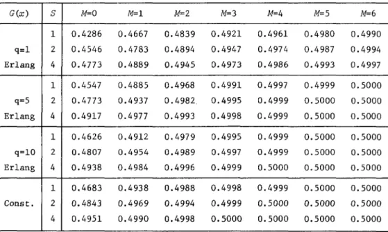
Tables 4.1 '" 3 show the production rates for the various parallel lines, where the operation times are given by q--Erlang or constant distribution with the mean 1/~. From these results it is appeared that the production rate increases as S increases but the rate of increase decreases and that the effect of S is larger when the buffer capacity M is small and the variance of the operation time is large. Furthermore in the unbalanced lines it is appeared that the production rate and the effect of S are larger and the rate of convergence to the maximum produetion rate yielded as M400 is fast when SA>~.

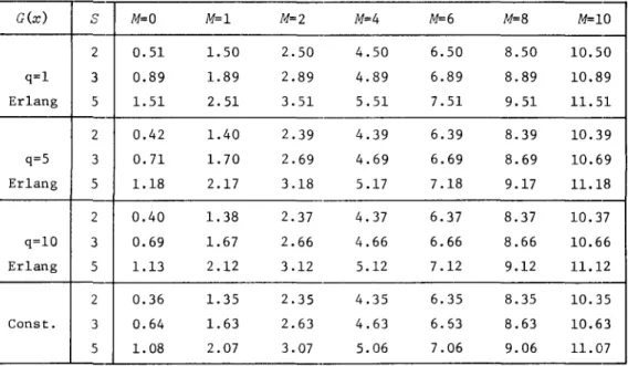
These situations can be simply explained by the imaginary buffer capacity

MI

as shown in Tables 4.4 '" 6, where the capacity

MI

is estimated by apply:Lng

the production rates of the series line to Newtons interpolation formula. That is, the imaginary capacity increases as S increases but the rate of

246 T. /yama

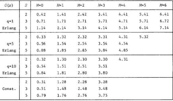
increase decreases, and the effect of S is large when q is small. Further-more, in the unbalanced l:ines, the imaginary capacity and the effect of S are larger when SA>~, and they are also larger than those for the balanced line.

Like this we can discuss the effect of the number of stations by the imaginary buffer capacity instead of the production rate, so that it is convenient to use this capacity if it is calculated by the easier procedure than that in Section 3. And, better still, it is expected that the imaginary capacity has the linear asymptote as M becomes large and that this asymptote gives the approximation value of MI within a small error for small M as well as large M. Therefore the effect of S can be discussed by this asymptote.

Now we present the procedure to estimate the asymptote on the assumption that G(x) is q-Erlang distribution with the mean l/~.

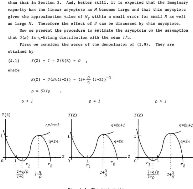
First we consider the zeros of the denominator of (3.9). They are obtained by (4.1) Y(Z) 1 - Z/K(Z) where K(Z)

=

U(SA(l-Z) p SA/~ p < 1

o

(1+~ (l-Z»-q q p 1 p > 1

Y(Z) Y(Z) Y(Z)

1 0 q=2n+l q=2n+l q=2n+l 1 Z Z 0 1 _Y'2 Y'l

Y'l Y'2 _Y'l Y'2

l+q/p _l+~ l+':! l+q/p _l+~

l+q p p

_1+P

p

Fig. 4.1 The real roots

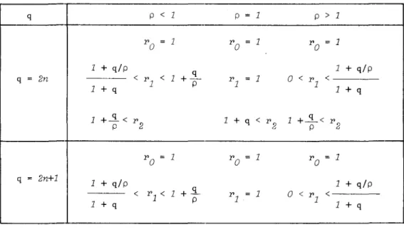
This equation has (q+l) roots but, as shown in Fig. 4.1, the number of the real roots is only two or three according to the value q. Therefore, if the roots are denoted by r. (i=O,1,2, .•• ,q) and especially the real roots

'l-The Efficiency of Two-Stage Line

are denoted by PO' P

1,P2 or PO' P1,the real roots exist in the range shown in Table 4.7 and we have (4.2) instead of (3.9),

(4.2) q A

+

--q-] 1 1--Z P q

where A. (i=1,2, ... ,q) is constant and E A.=l. From this equation P;

1.- i=l 1.- '"

(O~i~M) is given by

(4.3) P. = Po

i

A

(~)i

1.- t=l t Pt

247

Next, we consider the absolute value for the imaginary roots P. (i=2,3,

1.-... ,q or i=3,4, 1.-... ,q). By using w=l+(p/q)(l-Z), the equation (4.1) is re-written by (4.4) 2 q-l q, q (l-w) (1+w+w

+ ....

+w - -w ) p and hence (4.5) Z

=

1 (4.6) 3(1+e.(1-z»q = 1+(1+ '£'(1-Z»+ .•.. +(1+e.(1_Z»q-l p q q q

Equation (4.6) contains the imaginary roots, so that by calculating the absolute value we have

(4.7)

1

='£'1

1

+ .... +

1

q 1+e.(1-Z) (1+

e

(1-Z»q q q 2- .

..e.. (

1 1

1

+ .... +

1

__

1_1

q) - q l+~(1-Z) l+!?(1-Z) q q

where the equality is given by Z P

1• Therefore, if Z is a complex number, we have

(4.8)

248 T. /yama

This means that the absolute value for the imaginary roots is larger than r 1 which is minimum in the real roots besides rO=l.

On the other hand, by using (3.4), '¥k in (3.13) is (4.10) '¥ C ( S )M['l P +S

~

(S-k)i-1p .

k = S k S-k fO,k 0 O,k i~l S ~

- SO,k S+l

C

k

PM

'¥S

=

PM -

SO,?M+1 - SO,S S+l

C

S

PM

and hence, by substituting (4.3), this equation becomes

(4.11)

Furthermore from (3.13) HO is given by

S S-l i

(4.12) _HO 'IT <P_iP_{M -} l: 1jJ.+1 'IT <P .

i=l i=O ~ j=O J

1jJ.

~ '¥ ~ ./SO . ,~

1 -

So .

_,~

So .

_,~ (i=1,2, ... ,S) <Po = 1

and by substituting (4.11) we have

(4.13)

E.

~ i 'IT <p. j=l J

Therefore normalizing condition (3.15) gives the actual probability for

Po

The Efficiency of Two-Stage Line (4.14 ) M+1 S-l 1 q _{(-.2) i} q _(-.1...)M+2 S

Po

_t=l L: At _i=O L: 1't

+

_t=l L: A,Q, 1't _{1 - - -}S-l 1 S 1'£

Especially in the series line, i.e. S=l,

Po

is represented by

P

_Ol

(4.15) _1_ = P

Ol

Now we can solve the imaginary buffer capacity

M

I

.

In the above equation

Po

and

P

_Ol are the function of

M,

so that this imaginary capacity is given by the following equality;

(4.16) _R SA = POeM)

+

p SA and finally (4.17) 249

To estimate the asymptote for

Mr

let study the behavior of

Po

and

Pol

as

M

becomes large. From the discussion about the roots of (4.1), it is appeared that 1/1'1 has the maximum value among l/I1'i

l

(i=1,2, •.• ,q), so that (4.15) is rewri t ten as At Al l/1't M+2 1 q _(-.L)M+2 q At (l/1'l) } (4.18) POl L: 1 -{ - - + L: t=l 1 - - 1'1

1--~

t=2 1 __ 1_ 1't 1'1 1't and hence we have the asymptote for P

Ol as M becomes large as follows;

At 1 -(~)M+2 1 q 1'1 (4.19) - - - + _P L:

₊

_Al P ~ 1 Ol t=2 1 1 1 ___ 1_ 1'£ r'1 -+ p 1

250 T./yama

By the same way, (4.14) is rewri t ten as

(4.20) l/Y'l M+2 1 q Al _(..l.)M+2 A1 q Al (l/Y'/ 2: 1 { 1

+

2: 1 }

Po

_{l=l 1} Y'1 _{1 l=2 1}

Y'9v Y'1 Y'9v

S-l S-l

S _ " E C

S-l 1 i~l i S-l i

---S

Y'1

and we have the asymptote for

Po

as follows;

(4.21) q 2 : - -A9v +A 9v=2 1 1 1 1 1 ->-q A 9v 2: - - -

+

A (M+2) 9v=2 1 __ 1_ 1 Y'9v 5-1 1

+

A {S-l- 2: E. S l C . S . . }

l i=l 'I- - 'I- S(l-

~'I-)

(1- S-;-'l-)

The Efficiency of Two-Stage Line

Therefore, from (4.17), the asymptote for MI is given by the following simple equation; (4.22) 8-1 1 1 8 M +---=---'-1- log [1-(1- -){---c::'--::---::-log(-) 'P₁ 1- 8-1 1 ~ 8 ~ 8-1 i:1 Ei S_1Ci 8 i (i+1) p

+

1 p

=

1 251

This equation appears that the imaginary buffer capacity has the linear asymptote with the slope 1 as expected in Tables 4.4 'V 6. Furthermore, it appears that the asymptote is decided only by the minimum real root 'P

1 and, especially for p=1, this asymptote is completely decided since 'P

1=1. In Table 4.8, the asymptotes for the various production lines are represented. From the comparison between Table 4.8 and Tables 4.4 'V 6, it is appeared that the asymptote given by (4.22) presents the approximation values on the accuracy within 0.01 for M;;), so that this is very useful to evaluate the effect of S and also the other system parameters.

5. Conclusion

We have discussed the two-stage parallel line in which one of stages has a station but the other has S stations.

First, the procedure to estimate the, production rate is represented and the relations between the dual models are discussed. This appears that the dual models have the same production rate and the various characters for the one model can be derived from the: other dual model.

Next, we introduce the imaginary buffer capacity to evaluate the effect of the number of stations and show that the asymptote for the imaginary capacity can be obtained by the simple procedure and presents the good approximation value for the imaginary capacity. Therefore we can evaluate the effect of the number of stations by this asymptote.

252 T. /yama

Table 4.1 Production rate for the balanced line (l/SA= 111.1= 1.0)

G(x) S M=O M=l M=2 M=4 M=6 M=8 M=10 1 0.6667 0.7500 0.8000 0.8571 0.8889 0.9091 0.9231 q=l 2 0.7143 0.7778 0.8182 0.8667 0.8947 0.9l30 0.9259 Er1ang 4 0.7630 0.8084 0.8392 0.8783 0.9021 0.9182 0.9297 1 0.7133 0.8046 0.8525 0.9011 0.9256 0.9404 0.9503 q=5 2 0.7579 0.8266 0.8654 0.9071 0.9290 0.9426 0.9518 Er1ang 4 0.8021 0.8507 0.8804 0.9145 0.9334 0.9455 0.9539 1 0.7217 0.8138 0.8608 0.9076 0.9308 0.9447 0.9540 q-10 2 0.7653 0.8345 0.8727 0.9130 0.9339 0.9467 0.9554 Er1ang 4 0.8085 0.8574 0.8867 0.9198 0.9379 0.9493 0.9572 1 0.7311 0.8237 0.8696 0.9143 0.9362 0.9492 0.9578 Const. 2 0.7734 0.8431 0.8805 0.9192 0.9389 0.9509 0.9590 4 0.8154 0.8646 0.8934 0.9253 0.9425 0.9532 0.9606

Table 4.2 Production rate for the unbalanced line (1/SA=1.0, 1/~=2.0)

G(x) S M=O M=l M=2 M=3 M=4 M=5 M=6 1 0.4286 0.4667 0.4839 0.4921 0.4961 0.4980 0.4990 q=1 2 0.4546 0.4783 0.4894 0.4947 0.4974 0.4987 0.4994 Er1ang 4 0.4773 0.4889 0.4945 0.4973 0.4986 0.4993 0.4997 1 0.4547 0.4885 0.4968 0.4991 0.4997 0.4999 0.5000 q=5 2 0.4773 0.4937 0.4982. 0.4995 0.4999 0.5000 0.5000 Er1ang 4 0.4917 0.4977 0.4993 0.4998 0.4999 0.5000 0.5000 1 0.4626 0.4912 0.4979 0.4995 0.4999 0.5000 0.5000 q=10 2 0.4807 0.4954 0.4989 0.4997 0.4999 0.5000 0.5000 Er1ang 4 0.4938 0.4984 0.4996 0.4999 0.5000 0.5000 0.5000 1 0.4683 0.4938 0.4988 0.4998 0.4999 0.5000 0.5000 Const. 2 0.4843 0.4969 0.4994 0.4999 0.5000 0.5000 0.5000 4 0.4951 0.4990 0.4.998 0.5000 0.5000 0.5000 0.5000

The Efficiency of Two-Stage Line 253

Table 4.3 Production rate for the unbalanced line (1/SA=2.0, 1/~=1.0)

G(x)

S M=O M=l M=2 M=3 M=4 M=5 M=6 1 0.4286 0.4667 0.4839 0.4921 0.4961 0.4980 0.4990 q=l 2 0.4483 0.4754 0.4880 0.4941 0.4971 0.4985 0.4993 Er1ang 4 0.4653 0.4832 0.4918 0.4959 0.4980 0.4990 0.4995 1 0.4461 0.4821 0.4940 0.4980 0.4993 0.4998 0.4999 q=5 2 0.4625 0.4874 0.4957 0.4986 0.4995 0.4998 0.4999 Er1ang 4 0.4759 0.4918 0.4972 0.4991 0.4997 0.4999 0.5000 1 0.4489 0.4842 0.4951 0.4984 0.4995 0.4999 0.5000 q=10 2 0.4647 0.4889 0.4966 0.4989 0.4997 0.4999 0.5000 Er1ang 4 0.4775 0.4929 0.4978 0.4993 0.4998 0.4999 0.5000 1 0.4519 0.4864 0.4962 0.4989 0.4997 0.4999 0.5000 Const. 2 0.4670 0.4905 0.4973 0.4992 0.4998 0.4999 0.5000 4 0.4791 0.4939 0.4983 0.4995 0.4999 0.5000 0.5000

Table 4.4 Imaginary buffer capacity for the balanced line (l/SA= 1/~=1.0)

G(x)

S M=O M=l M=2 M=4 M=6 M=8 M=10 2 0.51 1.50 2.50 4.50 6.50 8.50 10.50 q=l 3 0.89 1.89 2.89 4.89 6.89 8.89 10.89 Er1ang 5 1.51 2.51 3.51 5.51 7.51 9.51 11.51 2 0.42 1.40 2.39 4.39 6.39 8.39 10.39 q=5 3 0.71 1.70 2.69 4.69 6.69 8.69 10.69 Er1ang 5 1.18 2.17 3.18 5.17 7.18 9.17 ll.18 2 0.40 1. 38 2.37 4.37 6.37 8.37 10.37 q=10 3 0.69 1.67 2.66 4.66 6.66 8.66 10.66 Er1ang 5 1.13 2.12 3.12 5.12 7.12 9.12 11.12 2 0.36 1.35 2.35 4.35 6.35 8.35 10.35 Const. 3 0.64 1.63 2.63 4.63 6.S3 8.63 10.63 5 1.08 2.07 3.07 5.06 7.06 9.06 11.07

254 T. Iyama

Table 4.5 Imaginary buffer capacity for the unbalanced line (1/SA=1.0,1/~=2.0)

G(x) S M=O M=l M=2 M=3 M=4 M=5 M=6 2 0.59 1.58 2.59 3.58 4.59 5.58 6.59 q=l 3 1. 08 2.08 3.08 4.08 5.08 6.08 7.08 Er1ang 5 1. 94 2.94 3.94 4.94 5.94 6.94 7.94 2 0.48 1.47 2.47 3.47 4.48 q=5 3 0.88 1.88 2.88 3.88 4.88 Er1ang 5 1.60 2.60 3.60 4.61 2 0.46 1.45 2.45 3.45 4.46 q=10 3 0.84 1.84 2.84 3.84 4.85 Er1ang 5 1.54 2.55 3.54 4.56 2 0.44 1.42 2.43 3.42 Const. 3 0.80 1. 79 2.80 3.79 5 1.47 2.48 3.46

Table 4.6 Imaginary buffer capacity for the unbalanced line (1/SA=2.0,1/~=1.0)

G(x) S M=O M=l M=2 M=3 M=4 M=5 M=6 2 0.42 1.41 2.42 3.41 4.41 5.41 6.41 q=l 3 0.71 1. 71 2.71 3.71 4.71 5.71 6.72 Er1ang 5 1.14 2.14 3.14 4.14 5.14 6.14 7.14 2 0.33 1.32 2.32 3.31 4.31 5.32 q=5 3 0.56 1.54 2.54 3.54 4.54 Er1ang 5 0.88 1.85 2.85 3.84 4.85 2 0.32 1.30 2.30 3.30 4.31 q=10 3 0.54 1.51 2.51 3.51 Er1ang 5 0.84 1.81 2.80 3.80 2 0.31 1. 28 2.28 3.28 Const. 3 0.51 1.48 2.48 3.48 5 0.79 1. 76 2.76 3.75

The Efficiency of Two-Stage Line 255

Table 4.7 The range in which the real roots exist

q p < 1 p = 1 P > 1 1'0 = 1 l' = 1 _{1'0 = 1} 0 1 + q/p 1 + q/p q = 2n < 1'1 < 1 +~ 1'1 = 1

o

< 1'1 < 1 + q P 1 + q 1 +2 < l ' _{1 + q < T'2} 1 +~< _1'2 P 2 p l ' 0 = 1 1'0 = 1 1'0 = 1 q = 2n+1 1 + q/p 1 + q/p < 1'1 < 1 +~ 1'1 = 1

o

< 1'1 < 1 + q P 1 + q

Table 4.8 The asymptote MI = M

+

a

a G(x) p S=2 S=3 S=4 S=5 S=lO 2.0 0.585 1.078 1. 524 1. 939 3.792 q=l 1.0 0.500 0.889 1. 219 1.510 2.660 Er1ang 0.5 0.415 0.711 0.945 1.141 1.825 2.0 0.471 0.876 1. 249 1.602 3.223 q=5 1.0 0.390 0.692 0.948 1.175 2.067 Er1ang 0.5 0.315 0.534 0.705 0.847 1.333 2.0 0.449 0.839 1. 200 1.543 3.126 q=10 1.0 0.371 0.660 0.905 1.122 1. 975 Er1ang 0.5 0.299 0.507 0.669 0.803 1.261 2.0 0.424 0.797 1.144 1.476 3.017 Const. 1.0 0.351 0.626 0.859 1.065 1.878 0.5 0.282 0.478 0.631 0.757 1.185

256 T. /yama

References

[I] Avi-Itzhak, B.: A Sequence of Service Stations with Arbitrary Input and Regular Service Times. Management Science, Vol. 11 (1965), 565-57l.

[2] Finch, P. D.: The Effect of the Size of the Waiting Room on a Simple Queue. Journal of the Royal Statistical Society, Vol. B-20 (1958), 182-186.

[3] Hashida, 0.: On the Busy Period in the Queueing System with Finite Capacity. Journal of the Operations Research Society of Japan, Vol. 15 (1972), 115-137.

[4] Hillier, F. S. and Boling, R. W.: The Effects of Some Design Factors on the Efficiency of Production Lines with Variable Operation Times. Journal of Industrial Engineering, Vol. 17 (1966), 651-658.

[5] Hillier, F. S. and Boling, R. W.: On the Optimal Allocation of Work in Symmetrically Unbalanced Production Line Systems with Variable Operation Times. Uxnagement Science, Vol. 25 (1979), 721-728.

[6] Iyama, T.: The Behavior of Some Design Factors in a Parallel Production Line. Journal of the Operations Research Society of Japan, Vol. 21

(1978), 226-243.

[7] Jain, H. C.: Queueing Problem with Limited Waiting Space. Naval Research Logistics (~uarterly, Vol. 9 (1962), 245-252.

[8] Knott, A. D.: The Inefficiency of a Series of Work Stations - A Simple Formula. International Journal of Production Research, Vol. 8 (1970), 109-119.

[9] Makino, T.: On a Study of Output Distribution. Journal of the Oper-ations Research Soc'iety of Japan, Vol. 8 (1966), 109-133.

[10] Suzuki, T.: On a Tandem Queue with Blocking. Journal of the Operations Research Society of Japan, Vol. 6 (1964), 137-157.

[11] Takacs, L.: On a Combined Waiting Time and Loss Problem concerning Telephone Traffic. Ann. Budapest Sect. Math., Vol. 1 (1958), 73-82. [12] Wild, R. and Slack, N. D.: The Operating Characteristics of 'Single'

and 'Double' Non-Mechanical Flow Line System. International Journal

of Production Resear'ch, Vol. 11 (1973), 139-145.

Toshirou IYAMA: Department of

Mechanical Engineering 11, Faculty of Engineering, Iwate University, 4-3-5, Ueda, Morioka 020, Japan