A Graphical Decomposition of the Stochastic Network

(1)

Journal of the Operations Research Society of Japan

Vol. 22, No. 2, J\lne 1979

A GRAPHICAL DECOMPOSITION

OF THE STOCHASTIC NETWORK

Noboru Yanagawa and Toshio Nishida Osaka university

(Received January 30,1978, Final February 9,1979)

Abstract The pivotal decomposition theorem of the reliability function is applied to the stochastic nNwork. A graphical observation of the theorem always yields more effective result than that of algebraic aspects, that is, the well· selected pivot arc enables the resulting network to contain modules. Our theorem 1 assures that, and our algorithms will be helpful to deTermine the optimal pivot of the decomposition.

1. Preliminaries

A network is said to be stochastic when its arcs either function or fail with known probabilit:les. Hereafter, the term network will refer to a

stochastic network satisfying following assumptions:

(AI) The network is an undirected network having the two specified nodes called terminals.

(AZ) Only arcs are subject to failure; nodes may not fail.

(A3) All arcs are relevant, that is, there is no arc whose deletion from the network will not affect its reliability.

(A4) The network can undergo no further modular decomposition, i.e. the network contains no modules having two or more arcs.

(AS) The state of each arc is statistically independent.

(A6) A graph obtained from the net'work by adding an artificial arc between the terminals is planar.

We deal with only nE!tworks as described above.

The reliability of a network is the probability that there exists a path from one terminal to anothE!r. We denote the arcs by 1,2, ... ,n, and its reli-ability (functioning probreli-ability) by Pi'

85

(2)

86 N. Yanagawa and T. Nishida

The reliability function h(p)

=

h(Pl"",Pn) is a multilinear polynomial of p. 'so The following lemna holds for h(p). (for the proof, see e.g. [1],

1. p.2l) Lemma 1. h(p) where (Pl"" ,Pi-l,l,Pi+l"" ,Pn) (P l ,··· ,Pi-1,O,Pi+l"" ,Pn) 1, ... ,n ,

A module is a subnetwork that acts as if it were just a component. If a network contains modules, we can replace each of them into single arc with the same reliabilities as that module has. These procedure are called "modular decomposition". The modula:r decomposition reduces the effort of calculat ion remarkably.

2. Graphical Representation of h(O.,p) and h(l.,p)

1 1

The following two propositions are obvious but important.

Proposition 1. The network N; representing h(Oi'P) is isomorphic to the network obtained by del,~ting an arc i from the original network N. Proposition 2. The network representing h(l. ,p)

1. is isomorphic to the network obtained by fusing both end nodes of an arc i of the origninal network N.

By these two propositions and lemma 1, the reliability function of the

i i

given network N is calculated from those of NO and Nl •

According to the assumptionB, N itself has no modules, however, the network i i

NO or Nl ' created from N, may be decomposable. In fact, we can prove the following:

Theorem 1. For any network N, there exists a pivot arc which produces the decomposable network

N~~

or

N~

•

Proof. Adding an arc between two terminals of the given network N, a planar graph G is constructed. By the proper transformation, G can be embedded in a plane such that every arc is drawn as a straight line segment. Therefore we can assume that G is such a graph as mentioned above.

Case 1. When G has at least one triangular region.

In this case, by fusing any two (except that those two are both terminals) of three nodes surrounding the triangular region, we can get the parallel arcs.

(3)

SrochG'stic Network 87

Hence is decomposable.

Case Z. When G has no triangular regions.

Let e,v, and f denote the number of arcs, nodes, and regions in G, respec-tively. Then Euler's formula holds irr e,v, and f;

(1)

f

=

e - v

+

Z.

Since G has no triangular regions, no region in G can be bounded with fewer than four edges. Hence we would have

(Z) Ze ~ 4f,

and, substituting for f from Euler's formula,

(3)

e ~ Zv -

4.

Let d (n

i) denotes the degree of nod.~ ni of the graph G, then

(4)

LV

d(n i)

=

Ze i=l from (3) and (4), -l\,v (5) v _{Li=l d(n i )} < 4 .

The assumptions (A3) and (A4) permit: neither series arcs nor pendant vertices, hence the degree of all nodes in G cannot be less than three;

(6) d(n

t) ~ 3 , for all i

The inequalities (5) and (6) show that there exists at least one node with degree thre.~, and if we remove an arc i from this node, a module of s.~ries

type is gen.~rated . (Two adjacent arCH are said to be in series i f thei>!; common node is of degree two.) Consequently Ni

°

is decomposable.

The fol101>1ing two examples illustrate our graphical decomposition proeedure. Example 1. The bridge structure.

2

₅

N

Applying lennna 1 to arc 3, the decomposable network N3 and N3 are

ob-°

1

tained. The reliability functions of

N~

and Ni are innnediate; h(03'P)

h(13' p)

PlP4

+

PZPs - PlP2 P4Ps

(PI

+

Pz - PlPZ)(P4

+

Ps - P4Ps) Hence the reliability function h(p) of N is

(4)

Example 2. The triangular frame.

s o----~.---Ot cr----~----~

2 5

N

Applying lemma 1 to arc 3, the decomposable networks

N~

and Ni are ob-tained. Ni can be reduced to the bridge structure of example 1, and the reliability functions of N3 and N3 are immediate;

°

1

(P1P6

+

P2 - P1P2P6) (P4 P7

+

PS - P4PSP7) , (1 - P6 - P7

+ P6P7) (P1P4

+ P2 PS - P1P2P4PS)

+

(P6

+

P7 - P6 P7)(P1

+

P2 - P1P2)(P4

+

Ps - P4PS) • Hence the reliability function h(p) of N is

h(p)

=

(1 - P3)h(03'P)

+

P3h (1 3,p) •

As was shown in above two examples, our graphical method is much efficient than other known methods such as path enumer~tion, state enumeration, and so forth. This is mainly due tc the possibility of decomposition of NO and N

1. Applying modular decomposition to the network reduces the computational effort especially.

3. Optimality of the Pivot Plrc

In applying our graphical decomposition to a given network, it is impor-tant that by which arc as a pivot the procedure is to be done. In this section we give a criterion for selecting a pivot arc of the decomposition. The term optimal means here that the number of states in the network are minimized. To this end, a concept of complexity of a network is proposed.

The complexity c(N) of the network N is considered to be a sort of measures that indicates the amount of the computational effort required to obtain its reliability function. And, the optimal pivot is defined as an arc i which gives the minimal sum of complexities for

N~

and

N~.

Birnbaum and Esary [2] formalized the concepts of module. In a wide sense, a single arc itself is a module however, we exclude this trivial case in the following discussions. We start from the definition of a level of the modules.

Let M

(5)

Stochastic Network

of the module Mi is defined recursiv.~ly as follows; (i)

(i i)

The whole network is a module with level zero. If Mi ::> M

j and there is no module ~ such that Mi ::> ~ ::> Mj , then the level of M

j is one greate:r than that of Mi; l(M

j)

= l(M

i)

+

1 .

89

(i i i)

The two modules M. and M. have the same level if no inclusion

rela-1. J

tion holds between those two. We say that Mi is higher level than I1

j i f the level of Mi is less than that of M

j • In the next, the complexity c(H) of a module M is defined as follows:

(i) If the module M with n arcs contains no submodules, then the complexity of M is 2n.

(ii) Let Sl"",Sk denote the submodules with level i

+

1 which are con-tained in the module M of level i . Then the complexity c(M) of M is given by

c(M)

=

c(M')

+

c(Sl)

+ ...

+

c(Sk) ,

where, M' is a module obtained from M, by replacing each of M's submodules SI"" ,Sk' respect:lvely, by a single arc.

*

Now, the optimality of arc i can be represented as follows: for i = l, ••. ,n •

4. Generation of Modules

We present some results helpful to determine an optimal pivot for the graphical decomposition. As in the previous sections, we use the symbol G for the graph obtained from the network N by adding an artificial arc between two terminals of N. The following p-ropositions 3 and 4 are from the proof of theorem 1.

Proposition 3. If there is a node w:lth degree three in the graph G, then by deleting an arc incident to that nod,~ we can get the series-type module in NO' Proposition 4. If G has a triangular region then by fusing any two of the three nodes constructing that triangle we can get the parallel-type module in NI'

In most cases we can find an optimal pivot by above propositions however, the more systematic method may be needed when the given network is complicated. We start from the discussion about some properties of the module. A knowledge of the concepts of regions is assumed. A graph theory text such as Deo [3] is recommended to those unfamiliar with these concepts.

(6)

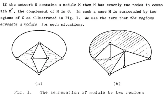
If the network N contains a module M then M has exactly two nodes in common with MC, the complement of M in G. In such a case M is surrounded by two regions of G as illustrated :in Fig. 1. We use the term that

the regions

segregate a module

for such situations.

(a) (b)

Fig. 1. The se~regation of module by two regions

The reformations of a module into two regions suggest to us a procedure to choose desirable pivots for our decomposition: If a subgraph S of N is segre~ gated by three reg:ions of G, and if these three satisfy some cond:itions then we can choose an arc whose d,:letion or shortage makes S a module in N. These considerations are described in two algorithms.

We define two relations Cl and i3 among the regions in the network.

(D1) For the two reg:ions R1 and R

2, we use the notation R1 Cl R2 if R1 and R2 are adj aeent each other.

(D2) For the two non·-adj acent regions R1 and R

2, we use the notation R1 i3 R2 if the boundaries of R1 and R2 have at least one node in common.

Algorithm 1. (for the deletion of arcs)

Step 1: Construct a planar graph G from the given network N by adding an artificial arc b,:tween two terminals of N.

Step 2: Let R

1, ... ,Rf denote the regions (including the outer region) of G. From f regions of G, select all the ordered triplets of

Step 3: regions (Cl) (C2) (C3) I f each

(R. ,R. ,R ) which satisfy one of the following conditons; 1. J -le Ri Cl R j , Rj Ri Cl R j , Rj Ri Cl R. , R. i3 J J

of the s.:lected triplet segregates a subgraph, then by deleting the arc which borders any two of the triplets a module is obtained.

(7)

Stochastic Network

Step 1: Construct a planar graph G from the given network N by adding an artificial arc between two terminals.

Step 2: Let Rl, ... ,R

f denote the regions (including the outer region) of G. From f regions of G, select all the ordered triplet of the

91

regions (Ri,Rj'~) which satisfy one of the following conditions;

Step 3: (Cl) (C2) (C3) (C4) I f each Ri CL R j , Rj Ri CL R j , Rj Ri CL R. , R. i3 J J Ri i3 R j , Rj i3

of the selected triplet

CL R. l. i3 R. l. i3 Ri i3 Ri

segregates a subgraph S, then S has just three nodes in co:nmon with its complement G - S (Le. the vertex attachment number of S is three). And if there is an arc between the two of these three nodes, then by shortening that arc a module is obtaiGed.

5. Discussion

The graphical decomposition is also applicable to some other problems such as maximum flow or minimum distance of the network. A slight modification of lemma 1 enables this.

Let F and c

i denote the flow from source to sink and the capacity of arc i, respectively. Note that the maximum flow is equal to the minimum of the capacities of all cut-sets. According to whether an arc i belongs to that minimal cut-set or not, the flow F can be expressed in two ways. These are concentrated as follows; F(c) where

Fe",.

,c) 1. (cl,···,ci_l,O, ... ,c n) (cl,···,c. l'oo, •.. ,c ) 1.- n

Similarly, let D and d

i denote the distances between two terminals and arc i, respectively, then the following equation holds;

D(d)

=

min ( D(ooi,d) , D(Oi,d)

+

d_i ) •

While the graphical method has many desirable effect, it has some limitations, too. We summarize them below.

(Ll) The pivot arc must be uGdirected.

(L2) The difficulty extremely increases when the network is non-planar.

(8)

not be treatl~d.

6. Supplementation

The following inequalities are obtained from the monotonicity of the re-liability function h(p).

h(Oi'P) ~ h(p) ~ h(li'P) , for all p and i •

Those inequalities show that the lower and upper bounds of the reliability of N can be calculated from those of Ni and Ni, respectively. We present

_o

1

a numerical example using above inequalities. The example is due to Shogan[4], and some arcs in the networ:~ are directed (as arrowed in the figure).

Shogan[4] also shows that hls sequential bounds are always tighter than Esary-Proschan bounds. The Esary·-Proschan bounds are presented in [1].

Shogan's network lower bound's network upper bound's network

Denote the exact reliability, the lower and upper bounds based on above inequalities, and Shogan's upper and lower bounds respectively by _R,~,~,RSL' and RSU' The following table exhibits those values corresponding to the various reliability of arcs. For the simplicity, we let the arc's reliability Pi=P for all arc 1.

p

_~

_RSL R _RSU

_~

0.1 .003 .001 .005 .005 .011 0.2 .029 .011 .042 .042 .075 0.3 .101 .056 .141 .158 .206 0.4 .229 .187 .305 .350 .385 0.5 .406 .411 .506 .575 .574 0.6 .605 .654 .700 .766 .742 0.7 .786 .838 .851 .890 .868 0.8 .917 .943 .945 .957 .948 0.9 .984 .988 .988 .990 .989

Since the bounding networks are limited, our bounding are less suitable for the directed network. I f t.he network is undirected, then our bounding will

(9)

Stochastic Network 93

become more powerful. We are convinced that our method provides the useful tools in reliability analysis because of its intuitive advantages, its ability of decomposition, and its flexibility of usages.

References

[1] Bar1ow, R. and Proschan, F.

Statistical Theory of Reliability and

Life Testing

Ho1t, Rinehart,

&

Winston, New York 1975.

[2] Birnbaum, Z.W. and Esary, J.D. ; "Modules of Coherent Binary Systems"

SIAM

J.

Appl. Math.

13 (1965) 444-462.

[3] Deo, N.

Graph Theory with Applications to Engineering and Computer

Science

Prentice-Hall, Inc., Engle'ioIood Cliffs, N.J. 1974.

[4] Shogan, A.W. : "Sequential Bounding of the Reliability of a Stochastic Network"

Opns. Res.

24 (1976) 1027-1044.

A Graphical Decomposition of the Stochastic Network