Robust Optimization Approach
to Network Congestion and
Power Efficient Network
Problems
Bimal Chandra Das
Department of Communication Engineering and Informatics
The University of Electro-Communications
Tokyo, Japan
A thesis submitted for the degree of
Doctor of Engineering
Robust Optimization Approach to Network Congestion
and Power Efficient Network Problems
APPROVED BY SUPERVISORY COMMITTEE:
Chairperson: Prof. Masakazu Muramatsu
Department of Computer and Network Engineering
The University of Electro-Communications, Tokyo
Member: Prof. Eiji Oki
Department of Communications and Computer Engineering
Kyoto University, Kyoto
Member: Prof. Yasushi Yamao
Advanced Wireless Communication Research Center
The University of Electro-Communications, Tokyo
Member: Prof. Yoshio Okamoto
Department of Computer and Network Engineering
The University of Electro-Communications, Tokyo
Member: Prof. Yusaku Yamamoto
Department of Computer and Network Engineering
The University of Electro-Communications, Tokyo
Member: Prof. Kitsuwan Nattapong
Department of Computer and Network Engineering
The University of Electro-Communications, Tokyo
Copyright
by
Bimal Chandra Das
March 2018
和文概要
本研究は、通信ネットワークの問題に対してロバスト最適化の手法を適用すること をテーマとしている。 1 つ目の題材は、基幹ネットワークが混雑しないようにルーティングを定める問題 である。基本的かつ重要な問題である。既存研究では、通信需要が正確にわかってい るモデルや末端ノードにおける入出力量が制限されているモデルなど、さまざまなモ デルが提案されている。この問題において通信需要が正確にはわかっていない場合を 想定し、真の通信需要が楕円体と多面体の交わりに含まれているという仮定のもとで ロバスト最適化の手法を適用し、その問題を2 次錐計画問題として定式化した。いく つかの例に対して数値実験を行い、提案したモデルは汎用ソルバーを用いて合理的な 時間内で求解可能であることを示し、また、従来のモデルとの比較検討を行なった。 2 つ目の題材は、エネルギーの節約のために不要なネットワークのリンクの電源を 落とす問題である。このとき、真の通信需要が正確にはわからない状況は容易に起こ りうるし、ネットワーク全体が通信需要のゆらぎに対して頑健であることが求められ る。真の通信需要が楕円体と多面体の交わりに含まれているという仮定のもとでロバ スト最適化の手法を適用し、その問題を整数2 次錐計画問題として定式化し、実際に 汎用最適化ソルバーで求解できることを示した。Abstract
This thesis focuses on providing robust optimization models for min-imization of the network congestion ratio and design of power effi-cient network that can handle fluctuation in traffic demands between source-destination pairs in the networks. It has become essential to design networks that are robust to di↵erent traffic conditions.
In the first part of the thesis, we propose robust optimization models to minimize congestion ratio for better performance of the network. The simplest and widely used model to minimize the con-gestion ratio, called the pipe model, is based on precisely specified traffic demands. However, in practice, network operators are often unable to estimate exact traffic demands as they can fluctuate due to unpredictable factors. To overcome this weakness, we apply robust optimization to the problem of minimizing the network congestion ra-tio. First, we review existing models as robust counterparts of certain uncertainty sets. Then we consider robust optimization assuming el-lipsoidal uncertainty sets; the total amount of squared errors in traffic demands is bounded by a positive constant which represents the to-tal admissible fluctuations over the network, and derive a tractable optimization problem in the form of second-order cone programming (SOCP). Furthermore, we take uncertainty sets to be the intersection of ellipsoid and polyhedral sets, and considering the mirror subprob-lems inherent in the models, obtain tractable optimization probsubprob-lems, again in SOCP form. Compared to the previous model that assumes an error interval on each coordinate, our models have the advantage of being able to cope with the total amount of errors by setting a parameter that determines the volume of the ellipsoid.
In the second part of the thesis, a green and robust optimiza-tion model is proposed to minimize the network power consumpoptimiza-tion. There are several researches that assume fluctuation in the traffic-demand matrix, our model is based on the idea of the green hose model where the knowledge of an exact traffic-demand matrix is not required. In the green hose model, the traffic is bounded by just total outgoing and incoming amount at each node. To allow fluctuations in traffic demands, here we also consider the same uncertainty set and subproblems as we did in the first part and formulate the green hose ellipsoid (green HE) model in the form of mixed-integer second-order cone programming (MISOCP) problem whose objective is to reduce the total energy by allowing some links to be put into the sleep mode. Furthermore, we establish a relationship between our model and the green HLT model, formulated from an extended version of the hose model called the hose model with bound of link traffic (HLT).
Numerical results demonstrate that our proposed robust op-timization models for congestion ratio and power efficient network achieves the performances with traffic fluctuations comparable to the previous studies in terms of congestion ratio, computation time and power efficiency.
Acknowledgements
This thesis is the summary of my doctoral study at the University of Electro-Communications, Tokyo, Japan. I am grateful to a large number of people who have helped me to accomplish this work.
First of all, I would like to express my sincere gratitude to my supervisor, Professor Masakazu Muramatsu, for his mentorship, guid-ance and encouragements. By working under the supervision of Pro-fessor Muramatsu, I received an invaluable experience that helped me to shape my academic and professional skills. I really feel very proud to be a student of his supervision. He showed me how to think and how to reach to the goal in a di↵erent way, which enhances my skills and makes this position. Secondly, I would like to thank Professor Eiji Oki for his continuous support, encouragement, and very useful guideline to develop my line of thinking for research. I also thanks to Professor Satoshi Takahashi for his help and useful comments to my research.
I would also like to thank, Professor Yasushi Yamao, Professor Yoshio Okamoto, Professor Yusaku Yamamoto, and Professor Kit-suwan Nattapong for being part of my judging committee and pro-viding their precious comments to improve my thesis.
I would like to thank my Japanese language teachers at the Uni-versity of Electro-Communications, the personnel of the Center for International Programs and Exchange and the International Student Office for their precious support during my stay in Japan.
Finally, I want to deeply thank to my parents, my wife, oth-ers member of my family, relatives, all of my friends, colleagues, the community of Bangali in Japan, and all of my lab mates.
Contents
List of Figures v
List of Tables vi
1 Introduction 1
1.1 Fluctuations of traffic demands . . . 2
1.2 Related work . . . 2
1.2.1 Problem of minimizing network congestion ratio . . . 2
1.2.2 Power efficient network problem . . . 4
1.3 Problem statement . . . 5
1.4 Contributions . . . 6
1.5 Organization of the thesis . . . 7
2 Network communications 9 2.1 Components of communication network . . . 9
2.1.1 Node . . . 9
2.1.2 Link . . . 10
2.2 Network model . . . 10
2.3 Di↵erent types of network . . . 12
2.3.1 Geographic spread of nodes and hosts . . . 12
2.3.2 Restricted access network . . . 12
2.3.3 Communication model employed by the nodes . . . 12
2.3.4 Switching model employed by the nodes . . . 13
CONTENTS
3 Second-order cone programming 14
3.1 Preliminaries . . . 14
3.2 Second-order cone programming . . . 15
3.3 Duality of conic linear programming . . . 18
3.4 Mixed-integer second-order cone programming (MISOCP) . . . . 22
4 Robust optimization 23 4.1 General form of robust optimization . . . 23
4.2 Robust optimization for linear programming with polyhedral un-certainty sets . . . 24
4.3 Robust linear programming with ball uncertainty sets . . . 26
5 Minimizing network congestion ratio with traffic fluctuations 28 5.1 Minimizing network congestion ratio and existing robust optimiza-tion models . . . 29
5.1.1 Problem formulation . . . 29
5.1.2 Hose model . . . 30
5.1.3 Hose-rectangle model . . . 33
5.2 Robust optimization models using ellipsoidal uncertainty set . . . 34
5.2.1 Ellipsoidal uncertainty set . . . 34
5.2.2 Ellipsoid model . . . 36
5.2.3 Hose-ellipsoid model . . . 38
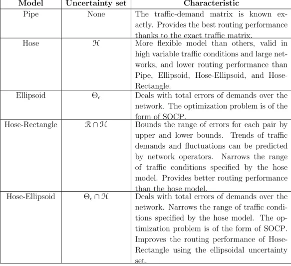
5.2.4 Characteristic of the considered models . . . 42
5.3 Numerical experiments . . . 42
5.3.1 Experiments settings . . . 42
5.3.2 Experiment results for fixed ✏ . . . 44
5.3.3 ✏ dependency of the models . . . 48
5.4 Summary . . . 50
6 Minimizing network power consumption based on robust opti-mization 52 6.1 Minimizing network power consumption . . . 53
6.1.1 Power model . . . 53
CONTENTS
6.1.3 Green hose model formulation . . . 55
6.1.4 Green HLT model formulation . . . 56
6.2 Green hose-ellipsoid model formulation . . . 59
6.3 Relation between ✏ and . . . 61
6.4 Numerical experiments . . . 62
6.4.1 Experiment settings . . . 62
6.4.2 Model comparisons . . . 64
6.4.3 ✏ dependency of G. HE model . . . 66
6.5 Summary . . . 66
7 Conclusions and future work 69 7.1 Conclusions . . . 69
7.2 Future work . . . 70
A
Derivation of traffic flow condition for destination node
71B
Proof of Lemma 2
72C
Dual transformation of the problem S(x
ij)
74D
Proof of Lemma 3
76E
Proof of Theorem 6
77Publications 78
List of Figures
1.1 Measurement of traffic demands . . . 3
2.1 Network topology . . . 11
3.1 Second-order cone in 3 dimension . . . 16
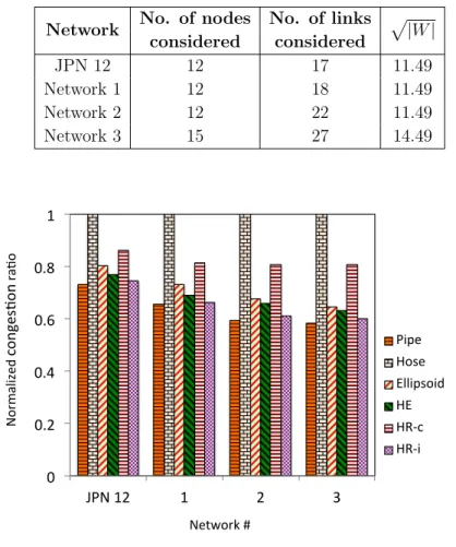
5.1 Sample networks . . . 44
5.2 Average normalized congestion ratio for 100 randomly generated problems for ✏ = 30. . . 45
5.3 Average normalized congestion ratio for 100 randomly generated problems for ✏ = 50. . . 46
5.4 Average normalized congestion ratio for 100 randomly generated problems for ✏ = 10. . . 47
5.5 Comparisons of average computation time of 100 randomly gener-ated problems for ✏ = 30. . . 48
5.6 ✏ dependency of congestion ratios for 100 random problems. Con-gestion ratios are normalized by the hose model (Network 3). . . . 50
6.1 Relation between ✏ and . . . 61
6.2 Sample networks. . . 64
6.3 Comparisons of power saving for = 0.5, ✏ = 24.75 (Network 1), 35 (Network 2), 95 (Network 3), 25 (Network 4). . . 65
6.4 ✏ dependency of G. HE model (Network 1). . . 67
6.5 ✏ dependency of G. HE model (Network 2). . . 67
List of Tables
5.1 Characteristic of models. . . 43 5.2 Network parameters considered in the experiments. . . 45 5.3 Comparisons of computation time of 100 randomly generated
prob-lems for ✏ = 30. . . 49 6.1 Summary of notations. . . 54 6.2 Network fixtures considered in experiments. . . 64 6.3 Number of deactivated links for = 0.5, ✏ = 24.75 (Network 1), 35
Chapter 1
Introduction
Nowadays, it is important to ensure an appropriate routing scheme in a network so that an operator can perform better in the case of traffic fluctuations due to various reasons and users’ need. In a backbone network, sending too much infor-mation on just a few of the links causes serious network congestion that results in greater end-to-end delay, packet loss, and decreasing the throughput. Network congestion can severely degrade the performance of the network [1]. Fortunately, setting an appropriate routing can enlarge the network resource utilization rate and the throughput [9]. Finding such a proper routing is a major concern for network operators whose goal is to provide better network performance.
The maximum link utilization rate among all links in a network is called the network congestion ratio [2]. Minimizing network congestion ratio is equivalent to maximizing additional admissible traffic [21].
Energy efficiency network is also a major concern in modern communication systems. Specially for economical and environmental reasons, energy-efficient networking has received a remarkable research interest over the last decade. The huge amount of power is consumed by the information and communication tech-nology (ICT) sector and it can save the worldwide energy by 2% to 10% [3], [4].
There are several researches on minimizing network power consumption that have been presented in the history. Most of them are presented under the as-sumption that the traffic-demand matrix, the set of traffic demands, is known and there are some bounds on the total outgoing/incoming traffic from/to node.
1. INTRODUCTION
Or, in addition to these bounds, traffic demands between each source and des-tination pair are bounded by upper and lower bounds [56]-[60]. There are also some studies on estimating the traffic-demand matrix, which makes it easy for network operators to avoid frequent dynamic route changes [61]-[63]. Most of the previous studies have a common objective to turn o↵ some links for green computing.
1.1
Fluctuations of traffic demands
The outgoing and incoming amount at each node in the network is defined as traffic. The traffic demand is denoted as the traffic volume that a source node requests to send to a destination node and the link capacity is the maximal volume of traffic that a link can accommodate. The traffic demands and link capacities are expressed in bits per seconds (bps). The set of demands which describes all the traffic demands between each source-destination pair in the network is called the traffic-demand matrix. When the network size is large, it is not easy for network operators to know the actual traffic matrix. In other words, since traffic demand between source and destination nodes easily fluctuates depending on the users’ needs, it is difficult task for network operators to compute the exact traffic-demand matrix. Therefore, it is challenging work for network operators to deal with the uncertain nature of traffic demands, if there are some errors in traffic demands. In the Figure 1.1, the matrix T which describes the traffic demands, dij for i = 1, 2, 3 and j = 1, 2, 3, is the traffic matrix. If there are some errors in
dij, then it is not so easy for operators to deal with this matirx.
1.2
Related work
1.2.1
Problem of minimizing network congestion ratio
There are several studies on the problem of minimizing the network congestion ratio. Wang and Wang [2] state that the problem of finding flows that minimize the network congestion ratio can be cast into a linear programming (LP) problem with the assumption that the traffic demand dpq for every pair of source node p
1.2 Related work
Figure 1.1: Measurement of traffic demands.
and destination node q, (p, q), is exactly known. This traffic-demand model is equivalent to the pipe model presented in [17], [18].
In practice, obtaining the exact traffic-demand matrix is difficult, if not im-possible, for network operators. In a typical situation, the network operators can only estimate the total outgoing/incoming traffic from/to each node rather than the actual traffic-demand matrix [13], [15]. Chu et al. [13] formulated the prob-lem of minimizing the network congestion ratio under this situation into an LP problem. Their traffic-demand model is called the hose model to contrast it with the pipe model [17], [18]. The hose model rids network operators of the heavy task of estimating the traffic-demand matrix exactly.
In general, the hose model has much lower routing performance than the pipe model. Based on the idea of additionally bounding the traffic demands in the hose model, Oki and Iwaki [20], [21] introduced another traffic-demand model that sets upper and lower bounds on the traffic demand between each pair of source and destination nodes in the network. They state that the problem of minimizing the network congestion ratio using their model can also be formulated as an LP problem. We call this model the hose-rectangle model in this paper as the bounded area for the traffic-demand matrix is contained in a rectangle.
1. INTRODUCTION
1.2.2
Power efficient network problem
In this thesis, we also propose another robust optimization model for minimization of the network power consumption. Minimizing the network power consumption is also ongoing research and there are lots of studies that have been presented in the history.
To minimize the power consumption in networks, Bianzino et al. [56] intro-duced the green pipe model based on the knowledge of previously specified traffic-demand matrix. The green pipe model achieves the high performance due to exact traffic demands. However, it may not be fully applicable in the case where the traffic demands often fluctuate.
In green computing, Ou´edraogo and Oki [30] applied the idea of the hose model introduced by Duffield et al. [17]. The hose model is contrary to the pipe model introduced by Wang and Wang [2] and does not require the exact traffic-demand matrix as the pipe model does. In the hose model, they bound the traffic with total outgoing and incoming amount of traffic at each node. The hose model is robust against traffic uncertainty and it is called a flexible service model.
Ou´edraogo and Oki [30] introduced the green HLT model under traffic uncer-tainty to achieve power saving in networks. The green HLT model is proposed on the idea of a model called the hose model with bound of link traffic (HLT) [31], which is the developed version of the hose model. In HLT, the authors as-sume that network operators are able to impose additional bounds on the traffic passing through each link. The traffic bound for each link is determined by total amount of traffic measured on that link. Since the performance of the model depends on the maximum amount of traffic measured on each link, In the green HLT model, the authors proposed a parameter which indicates uncertainty to maximum amount of traffic measured on each link in order to maintain the ro-bustness in the model. In the green HLT model, the additional bound on link fixes the range of traffic demand described by the hose model and makes it close to the pipe model.
1.3 Problem statement
1.3
Problem statement
Based on the previous work related to the congestion ratio problem and power efficient networks, using the formulations based on the knowledge of the exact traffic information (pipe model) makes it possible to achieve significant perfor-mance in both cases. However, these approaches, apart from the difficulty of traffic prediction for operators, have weaknesses in face of traffic fluctuation. A scheme applying the hose model, on the other hand, provides robustness against traffic uncertainty, but meager routing and energy performance compared to the pipe model. The limitation with the hose model, which is highly conservative, is due to the wide range of traffic specification considered. On the other hand, the hose-rectangle model is also robust and provides better routing performance by adding additional bounds to the traffic demand for each pair. The hose-rectangle model has a weakness, that is, it does not deal with total fluctuation over the network except fluctuation in each pair.
In the case of power efficient network, the green HLT model is also robust against traffic uncertainty. In the green HLT model, the authors bound the traffic passing through each link by total amount of traffic measured on that link as an additional bound to the hose model. The performance of the green HLT is closed to the green pipe model due to additional bound for each link. But the green HLT requires initial routing to compute the total traffic measured on each link and the routes need to be changed after solving the optimization problem which is not preferable for additional operating procedures needed to maintain network stability.
Our goal is to provide robust optimization models in the form of SOCP for minimization of congestion ratio and power efficient network, where we can use an ellipsoidal uncertainty set to allow total amount of fluctuation over the network without any additional bound and enhance the performances compared to the pervious studies. This is the objective in this thesis.
1. INTRODUCTION
1.4
Contributions
This thesis introduces robust optimization models to minimize the network con-gestion ratio and for the design of power efficient networks allowing fluctuations in traffic demands between source-destination pair in the network. The assump-tion is that the network operator can estimate the traffic-demand matrix, but the estimated values may contain some errors where the total amount of er-ror is bounded by a predefined constant. In other words, we assume that the traffic-demand matrix is contained in some uncertainty set whose ‘center’ is the estimated traffic-demand matrix and whose volume is bounded by some constant. This is a relevant situation if we remember that estimating the traffic-demand matrix exactly is a virtually impossible task. Our models allow the network op-erator to roughly estimate the traffic-demand matrix, and indicate the amount of admissible error.
In the first part of this thesis (Chapter 5), we apply robust optimization to minimize the network congestion ratio with traffic fluctuation. To do this, we consider an ellipsoidal uncertainty set, di↵erent from the hose and hose-rectangle uncertainty sets. Here we propose two models. The ellipsoid model considers only the ellipsoidal uncertainty set, and the hose-ellipsoid model considers both the hose and ellipsoidal uncertainty sets. We derive robust counterparts for these models which turn out to be SOCP problems. To derive the robust counterpart of the hose-ellipsoid model, we exploit the duality of conic linear programming in the presence of polyhedral cones [41].
In contrast to the hose-rectangle model, which considers the error of each source/destination pair, our ellipsoidal uncertainty set allows us to manage just the total amount of error among all pairs. The ellipsoidal uncertainty set is especially appropriate when the network-wide demands are governed by a multi-variate gaussian probability distribution whose average is the estimated traffic-demand matrix.
It is well-known that, in general, a robust counterpart of LP with an ellipsoidal uncertainty set becomes an SOCP [24]. Our first model, the ellipsoid model, follows this logic; the original model is an LP, and we consider the ellipsoidal uncertainty set used to derive its robust counterpart as an SOCP. However, in the
1.5 Organization of the thesis
second model, the hose-ellipsoid model, we consider the intersection of polyhedral and ellipsoidal sets as an uncertainty set. Deriving a robust counterpart in such a case is non-obvious, but we are able to derive it as an SOCP by applying the duality theorem of SOCP. This is our major contribution.
In the second part of this thesis (Chapter 6), we propose a green and robust optimization model to the problem of minimizing the network power consump-tion using the same ellipsoidal uncertainty set that can also deal with traffic fluctuations. Our model introduced in that chapter is based on the hose-model-based optimization in green research applying second-order cone programming (SOCP) [16]. Our ultimate goal is to reduce the power consumption in networks by turning o↵ some unnecessary links under traffic fluctuation. To do this, we use an ellipsoidal uncertainty set in addition to the hose model traffic bounds, where we assume that the true traffic-demand matrix is contained in the uncer-tainty set whose center is the estimated traffic-demand matrix and whose volume is bounded by some constant which indicates the total amount of fluctuation over the network
For robust optimization, we consider subproblems for the worst-case traffic scenario taking the uncertainty set which is the intersection of ellipsoidal and polyhedral sets. The subproblem is changed into a tractable SOCP problem. Finally using the knowledge of conic duality of the subproblem, we formulate the green hose ellipsoid (green HE) model again in mixed-integer second-order cone programming (MISOCP) form. Our proposed model allows the network operator to roughly estimate the traffic-demand matrix and represents the amount of permissible errors in the traffic demands.
1.5
Organization of the thesis
In Chapter 2, we discuss network communication with components of network, network model, and di↵erent types of network. Basic concept of conic program-ming and its dual are described in Chapter 3. In the later part of Chapter 3, we briefly discuss about mixed-integer second-order cone programming. The robust optimization with uncertainty sets are described in Chapter 4.
1. INTRODUCTION
Chapter 5 presents the robust optimization model for the problem of mini-mizing the network congestion ratio. In this chapter, first we explain the pipe model, which demands the exact traffic-demand matrix, and then, we show that the hose and hose-rectangle models can be viewed as robust counterparts of the pipe model. After introducing the ellipsoidal uncertainty set that we use in our models, we formulate the ellipsoid model, the hose-ellipsoid model, and derive their robust counterparts.
In Chapter 6, another robust optimization model is presented in order to min-imize the network power consumption for green computing considering the traffic uncertainty. The power model used to build the model is first introduced. Then the steps, which lead to the MISOCP formulation of green HE, are explained in details using the same uncertainty set as we used for formulation of the HE model in Chapter 5. These steps include the formulation for known traffic de-mands (green pipe model) and the formulation of the green hose model and green HLT models using the respective uncertainty sets.
The performances of our proposed models for congestion ratio and power efficient network are shown in experiments sections at the end of Chapter 5 and Chapter 6, respectively. We have conducted the experiments to check whether the proposed models can be solved in a reasonable time or not. In particular, in the case of MISOCP, there is a possibility that the problem cannot be solved in a reasonable time because it is NP-hard. The another reason for experiments is to observe some properties of the proposed models with respect to other models numerically. Some properties are proved in theory, but some are not proved.
Chapter 7 concludes the thesis by summarizing the findings and showing the direction for future work.
Chapter 2
Network communications
A communication network is an infrastructure that allows two or more nodes to communicate each other. The network accomplishes this by arranging a set of rules for communication, which are called protocols that should be observed by all participating nodes. In this chapter we review the fundamental concept of network communication. We will first discuss the constituent network compo-nents and various types of network, and then introduce the network model and backbone network.
2.1
Components of communication network
2.1.1
Node
A node is a point or vertex where more than two branches (links) meet. In a general communication network, there may be a large number of nodes and it is not necessary that each of them is connected to all others. The nodes typically handle the network protocols and provide switching capabilities. A node is usually itself a computer (general or special) which runs specific network software. The computers are also called the hosts of the network. The function of a network node is to make a connection between the output and incoming paths so that the signal can be switched to the desired path for onward transmission. In a telephone network, the telephone exchange (circuit switch) works as a node. In a data network, packet switch is known as node and is usually indicated to as a
2. NETWORK COMMUNICATIONS
router. There are some nodes, like the message and packet switching ones, that have bu↵ers and storage for messages. These kinds of nodes work as store-and-forward switches. There are also other functions of nodes like determining the incoming message, testing the free outlet, signaling, etc.
In a communication network, there are two kinds of nodes: edge node and intermediary node. The function of an edge node is to admit the data into the network and forward the data from one network to another network. The function of an intermediary node is to receive and forward data from one node to another node.
2.1.2
Link
The transmission medium of a communication network is known as a link which can be either a wire or a radio channel. There are di↵erent kinds of wired trans-mission medium such as a co-axial cable, an optical fiber, pair of copper wires or a multi-pair cable. The above transmission medium broadcasts the signals from one node to the other. The wireless transmission medium is a part of electromag-netic spectrum ranging from very low frequency to ultra high frequency including millimeter and optical waves. The wireless and wire channels can support data rates ranging from a few bits per second to many Giga/Peta bits per second since they have a very wide range of bandwidth. Due to various reasons such as dis-persion and attenuation, the lengths of these transmission links are limited. All kinds of links in a communication networkIt are not necessary to be of the same type. Some of them can be wireless and some other may be wired.
2.2
Network model
A network interconnects many nodes through which a desired entity flows. The network is expressed as a directed graph G(V, A), where A is the set of links and V is the set of nodes. Let the set Q ✓ V represents the set of edge nodes through which data is admitted into and going outside the network. In this thesis, an edge-node pair of p 2 Q and q 2 Q, where p 6= q, is denoted by (p, q) 2 W , where W indicates the set of edge-node pairs (p, q). The link from
2.2 Network model
node i2 V to node j 2 V \ {i} is represented as (i, j) 2 A, i 6= j. Here cij and uij
represent the capacity and the flow on (i, j)2 A, respectively. We consider the full duplex links in this research and both directions are powered on when there is data in one direction. Deactivating a link between node i and node j means deactivating both directions (i, j) and (j, i). The binary variable bij represents
the on/o↵ status of the links. The orientation of link remains di↵erent in the mathematical formulation although both directions (i, j) and (j, i) are powered on or o↵ simultaneously. Power consumption of (i, j) 2 A is an affine function of its usage (ratio between its load and capacity). Here Ef ij is the slope of the
function and E0ij is the constant term. The consumption of a link is equal to E0ij
when it is powered on and does not hold any traffic. The set of traffic demands is represented by T ={dpq}. And xpqij, where 0 x
pq
ij 1, is the portion of the
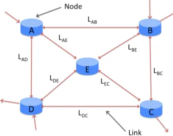
traffic from p2 Q to q 2 Q\{p} routed through (i, j) 2 A. Figure 2.1 describes a network topology with five nodes A, B, C, D, and E. These nodes are connected with the links LAB, LBC, LDC, LDE, etc.
2. NETWORK COMMUNICATIONS
2.3
Di↵erent types of network
Based on the following four criteria the networks are divided into di↵erent types.
2.3.1
Geographic spread of nodes and hosts
Local area network (LAN): A network is said to be a Local Area Network (LAN) if the physical distance between the hosts is within a few kilometers. LANs are usually used to connect a set of hosts within the same building e.g., an office environment or a set of closely-located buildings e.g., a university campus. Metropolitan area network (MAN): For larger distances, the network is said to be a metropolitan area network (MAN) or a Wide Area Network (WAN). MANs interconnect hosts across a city and cover distances of up to a few hundred kilometers.
2.3.2
Restricted access network
Private network: The network where the users are supposed to use the service for their private or business purpose. Networks maintained by banks, insurance companies, airlines, hospitals, and most other businesses are of this nature. Public network: The network where the users have to complete required regis-tration and have to pay the connection fees to get access to the network. Internet is the well known example of public networks.
2.3.3
Communication model employed by the nodes
Point-to-point model network: In this network, to get access from one node to another the message or information has to follow a specific route.
Broadcast model network: In this network, all nodes share the same commu-nication medium. Therefore, a message or information transmitted by any node can be received by all other nodes. A part of the message (an address) shows for which node the message is designed and the nodes ignore the message if it does not match their own address.
2.4 Backbone network
2.3.4
Switching model employed by the nodes
Circuit switching network: In circuit switching network, a dedicated com-munication path is allocated between two hosts to communicate each other in the network, via a set of intermediate nodes. The information is sent through the path as a continuous stream of bits. This path is maintained for the duration of communication between two nodes, and is then released.
Packet switching network: To send information form one node to another, packet switching network divides the information into packets and also uses in-termediate nodes to pass the information. Each inin-termediate node temporarily stores the packet and waits for the receiving node to become available to receive it. Since data is sent in packets, it is not necessary to reserve a path across the network for the duration of communication between two nodes. In order to en-hance the performance of the network, di↵erent packets can be routed di↵erently to spread the load between the nodes. However, this requires packets to allow additional admissible information.
2.4
Backbone network
The backbone network interconnects various local networks and provides paths for the exchange of information between them. It can tie together diverse networks in the same area, in di↵erent areas, or over wide areas. A large corporation that has many locations may have its own backbone network that ties all of the locations together. The network transmission medium such as ethernet, wire or wireless connections that bring these location together is often mentioned as network backbone. It is important to consider the network congestion while designing the backbones for better performance of the network.
Chapter 3
Second-order cone programming
The importance of second-order cone programming (SOCP) and mixed-integer second-order cone programming (MISOCP) problems has long been a focus of the mathematical programming society. In this chapter, we discuss basic concepts of SOCP and MISOCP with related propositions and theorems to read this thesis.
3.1
Preliminaries
In this subsection, we list some definitions needed for the following discussions.
Definition 1 A set C ✓ Rn is a cone if and only if for any positive scalar and
for any x2 C it holds that
x2 C.
Definition 2 Let C ✓ Rn. Then C is convex if for any two points x
1, x2 2 C, it
holds that,
✓x1+ (1 ✓)x2 2 C, 8 0 ✓ 1.
Let C be a convex set inRn. A function f : C ! R is said to be a convex function
if 8x1, x2 2 C it holds that
f ( x1 + (1 )x2) f(x1) + (1 )f (x2), 8 0 1.
Definition 3 A set S ✓ Rn is affine if x
1, x2 2 S implies that
3.2 Second-order cone programming
for every real number t. Geometrically, a set is affine if whenever two points are in the set, the entire line through these points is in the set. An affine combination of vectors is a special kind of linear combination. For given vectors, v1, v2, . . . , vm 2
Rn and scalars c
1, c2, . . . , cm an affine combination of v1, v2, . . . , vm is a linear
combination c1v1+ c2v2+· · · + cmvm such that c1+ c2+· · · + cm= 1.
Definition 4 An open ball of radius ✏ is the set of points of distance less ✏ from a fixed point. The open ball centered at x and radius ✏ is defined by
B(x, ✏) ={y : ||y x|| < ✏}.
Definition 5 The set of all affine combinations of vectors in a set S is called the affine hull of S, and it is denoted by a↵(S).
Definition 6 A point x2 C is a relative interior point of C if there exists ✏ > 0 such that B(x, ✏)\a↵(C) ✓ C. The set of relative interior points of C is the relative interior of C, denoted by ri(C).
Definition 7 An optimization problem of the form
minimize f (x) (3.1a)
s.t. gi(x) 0, i = 1, 2, . . . , m, (3.1b)
is said to be a convex optimization problem if the functions f, g1, . . . , gm :Rn! R
are convex.
Definition 8 Given an optimization problem P , we call a solution x feasible for P if it satisfies all the constraints of P . When f is the objective function of the optimization problem P , we define
val(P ) = inf{f(x) : x is feasible},
which will be called the optimal value, or value of the optimization problem P .
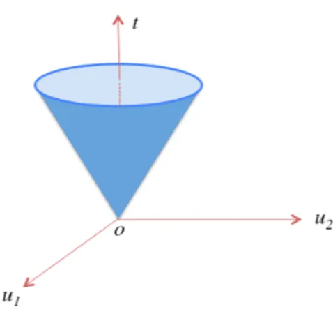
3.2
Second-order cone programming
The second-order cone (SOC) of dimension l + 1 is defined as SOC(l + 1) = ⇢✓ t u ◆ : u2 Rl, t2 R, ||u|| t , (3.2)
3. SECOND-ORDER CONE PROGRAMMING
Figure 3.1: Second-order cone in 3 dimension.
which is also called the quadratic, ice-cream, or Lorentz cone. A second-order cone of dimension 3 is presented in Figure 3.1. The unit second-order cone of dimension 1 is defined as
SOC(1) = {t : t 2 R, 0 t} .
It is easy to verify that SOC(l + 1) is a convex cone. The proof is presented below using the following Lemma 1:
Lemma 1 . Suppose C is a cone. Then C is convex if and only if
8x, y 2 C and 8 , µ > 0, x + µy 2 C. (3.3) Proof: If (3.3) holds, then C is obviously convex. Suppose C is a cone and convex, and x, y2 C and , µ > 0 are given. Since C is a cone, we have
+ µx2 C and µ
+ µy2 C. Since C is convex, we have
+ µx + µ
+ µy2 C.
Again since C is a cone, we can write x + µy2 C. Therefore, (3.3) holds. ⇤
3.2 Second-order cone programming
Proposition 1 SOC(l+1 ) is convex. Proof: Let x = ✓ t1 u1 ◆ 2 SOC(l + 1) and y = ✓ t2 u2 ◆ 2 SOC(l + 1). We have to show 8 , µ 0, || x + µy|| t1+ µt2.
For every, , µ 0 we can write
|| x + µy||2 = 2||x||2+ 2 µxTy + µ2||y||2
2||x||2+ 2 µ||x|| ||y|| + µ2||y||2
2t2
1+ 2 µt1t2+ µ2t22 = ( t1+ µt2)2,
which shows that ✓
t1+ µt2
x + µy ◆
2 SOC(l + 1). Therefore, SOC(l + 1) is convex. ⇤ Let K be a closed convex cone in Rn. Then K⇤ ={s : sTx 0 (8x 2 K)} is
called the dual cone of K. It is easy to see that K⇤ is in fact a cone. Furthermore,
we have the following property.
Theorem 1 (Separation theorem (cone version)) [39]
Let K be a closed convex cone and z /2 K. Then, there exists y such that yTz < 0 yTx, 8x 2 K.
Proposition 2 If K is a closed convex cone, then K⇤⇤ = K. Proof: Let x2 K. Then for every y 2 K⇤, xTy 0. So x 2 K⇤⇤.
Conversely, let ¯x 2 K⇤⇤. Then for every y 2 K⇤, ¯xTy 0. Suppose that
¯
x /2 K. Since K is a closed convex cone, according to the Theorem 1, there exists a vector ¯y such that
¯
yTx < 0¯ ¯yTx, 8x 2 K.
The right inequality implies that ¯y 2 K⇤. Then ¯yTx < 0 contradicts the fact¯
that ¯x2 K⇤⇤. Therefore, ¯x2 K.
3. SECOND-ORDER CONE PROGRAMMING
The dual of a second-order cone is itself, i.e., SOC(l + 1)⇤ =SOC(l + 1) [55].
Such a cone is called self-dual.
Second-order cone programming (SOCP) is a convex optimization problem in which a linear function is minimized over the intersection of an affine set and a direct product of second-order cones. The following is called the equality standard form second-order cone programming problem:
minimize cTx (3.4a)
s.t. Ax = b, (3.4b)
x2 K, (3.4c)
where x2 Rnis the decision variable, K ✓ Rnis a direct product of second-order
cones, and the other problem data are c2 Rn, A 2 Rm⇥n, and b2 Rm. To fully
understand the properties of SOCP, please consult [55] or textbooks such as [35], [52], [53], [54].
An SOCP can be solved efficiently by the primal-dual interior-point methods [48], [49], [50], [51]. In fact, Gurobi [38] can be considered as one of the standard solvers, such as CPLEX [43] and SCIP [42]. CPLEX and SCIP also support SOCP.
3.3
Duality of conic linear programming
SOCP is a subcategory of more general class of optimization problems called conic linear programming. In this section, we briefly review conic linear pro-gramming and its duality, and derive a dual of SOCP in a special form. This dual relationship is used to derive the dual of the problem S(xij) in Section 5.2.3
of Chapter 5.
We start with considering two closed convex cones C ✓ Rm and K ✓ Rn.
With ¯A 2 Rm⇥n, ¯b 2 Rm, and ¯c 2 Rn, we consider an optimization problem of
the form:
(P ) : min ¯cTx
s.t. Ax¯ b¯ 2 C, x2 K.
3.3 Duality of conic linear programming
This problem is called conic linear programming problem. Obviously, SOCP (3.4) is a special case of conic linear programming where C = {0} and K is a direct product of second-order cones. The (conic) dual of (P ) [40] is
(D) : max ¯bTy
s.t. ¯c A¯Ty2 K⇤, y2 C⇤.
It is easy to see that the weak duality holds between (P ) and (D).
Theorem 2 (Weak Duality) If x is feasible for (P ) and y for (D), then we have ¯cTx b¯Ty.
Proof: We can write
¯cTx b¯Ty = ¯cTx yTAx + y¯ TAx¯ b¯Ty
= (¯c Ay)¯ Tx + ( ¯Ax b)¯ Ty 0,
since ¯c Ay¯ 2 K⇤, x2 K, ¯Ax b¯ 2 C, and y 2 C⇤.
⇤ If C ={0} and K is a closed convex cone, then the primal-dual pair of conic linear programming becomes
(P0) : 8 < : min ¯cTx s.t. Ax = ¯¯ b, x2 K dual ! (D0) : ⇢ max ¯bTy s.t. ¯c A¯Ty2 K⇤.
The problem (P0), sometimes called the equality standard form of conic linear
programming, is widely used in the literature. Note that, although the rest of this section writes the theorems in terms of (P0) and (D0), all are also valid on
(P ) and (D).
We say (P0) satisfies Slater’s condition if there exists a feasible solution ¯x
such that
¯
3. SECOND-ORDER CONE PROGRAMMING
Similarly, we say that (D0) satisfies Slater’s condition if there exists a feasible
solution ¯y of (D0) such that
¯c A¯Ty¯ 2 riK⇤.
In conic linear programming, we need Slater’s condition to state the strong du-ality.
Theorem 3 (Strong Duality) [41]
1. If (P0) satisfies Slater’s condition, and (D0) has a feasible solution, then
val(P0) = val(D0), and (D0) has an optimal solution.
2. If (D0) satisfies Slater’s condition, and (P0) has a feasible solution, then
val(P0) = val(D0), and (P0) has an optimal solution.
Using the duality of (P ) and (D), we can easily show that the following theorem holds.
Theorem 4 Suppose that K is a direct product of SOCs, and b 2 Rm, A 2
Rm⇥n1, B 2 Rm⇥n2, c2 Rn1, f 2 Rn2. Then the dual of (P1) : max bTy s.t. ATy c, BTy = f , y2 K is (D1) : min cTx + fTw s.t. Ax + Bw b2 K, x 0.
Proof: The problem (P1) can be written as
max bTy
s.t. c ATy2 Rn1
+, (3.5)
3.3 Duality of conic linear programming
y2 K. (3.7)
Using the direct product Rn1
+ ⇥ {0}, we can write the above problem as
(P2) : max bTy s.t. ✓ c f ◆ ✓ AT BT ◆ y2 Rn1 + ⇥ {0}, y2 K.
If we compare the problem (P2) with problem (D), then we obtain the following
correspondence: ¯ A = ✓ AT BT ◆T = (A B)2 Rm⇥(n1+n2), ¯c = ✓ c f ◆ 2 R(n1+n2) + , and C = K.
Since K is self-dual, the dual of the problem (P2) is as follows:
min ✓ c f ◆T ✓ x w ◆ s.t. (A B) ✓ x w ◆ b2 K ✓ x w ◆ 2 Rn1 + ⇥ Rn2 , min cTx + fTw s.t. Ax + Bw b2 K, x2 Rn1 +, w 2 Rn2 , min cTx + fTw s.t. Ax + Bw b2 K, x 0,
which is the final dual form of (P2).
3. SECOND-ORDER CONE PROGRAMMING
3.4
Mixed-integer second-order cone
program-ming (MISOCP)
An MISOCP is an optimization problem which involves some real and integer variables to optimize a linear objective function subject to some linear and second-order cone constraints. It is well known that MISOCP is NP-hard and it is not so easy to solve MISOCP like LP or SOCP, because MISOCP involves integer variables in addition to the properties of LP or SOCP. Modern optimization software like Gurobi [38] and CPLEX [43] can handle MISOCPs but generally it takes longer computation time compared to LP or SOCP of a similar size.
Mixed-integer second-order cone problems have various applications in finance and engineering. For example, MISOCP have been used to model and solve many challenging applied problems such as transmission in cellular networks [5], power distribution [6], portfolio optimization [7], battery swapping stations on freeway networks [8], telecommunication network design [30], etc.
Chapter 4
Robust optimization
In the last few decades, the idea of robust optimization has emerged as a key trend in the field of optimization [22], [37]. In this chapter, we discuss the basic concept of robust optimization that we apply in this research.
4.1
General form of robust optimization
If some information of an optimization problem is not defined exactly, but it is said to belong to a predefined set ,and we want to optimize the problem in the worst case with respect to the set, then the resulting optimization problem is called a robust optimization problem ([23], [39], [52], [54]). The objective of robust optimization is to optimize the problem in the worst case wherein the problem data lie in a set. In such cases, the set where parameters are supposed to fall in is called uncertainty set. In general, the uncertainty set contains infinitely many points. This means that the robust optimization problem can be categorized as an instance of semi-infinite programming, which is inherently intractable. Thanks to the progress in conic linear programming, robust optimization is now being used in many real-world applications such as finance [44], mechanics [45], and control [46], [47] etc.
The general form of robust optimization problem can be stated as follows:
minimize f0(x) (4.1a)
4. ROBUST OPTIMIZATION
where x 2 Rn is a vector of decision variables, f
0, fi : Rn ! R are functions,
di 2 Rki are parameter uncertainties, and ⌦i are uncertainty sets. We can always
take the objective function to have no uncertainty by introducing a new constraint if necessary. The aim of the problem (4.1) is to compute minimum solutions x⇤ among all those solutions which are feasible for all realizations of the di 2
⌦i. The optimization problem (4.1) o↵ers some measure of feasibility protection
for optimization problems containing parameters which are not known exactly. Although a robust optimization problem is in general intractable, in some cases, we can reformulate it as a conic linear programming problem which is tractable, and this is the case we present in the thesis. In such a case, the reformulated optimization problem is called robust counterpart.
In the following sections, we consider robust optimization for LP. We con-sider two uncertainty sets: a polyhedral uncertainty set and a ball uncertainty set. We present how we can derive robust counterparts of the robust linear pro-gramming. In the latter chapters, similar arguments will be used to obtain robust counterparts of various models.
4.2
Robust optimization for linear programming
with polyhedral uncertainty sets
The linear programming (LP) problem can be represented as min
x c
Tx (4.2a)
s.t. aTi x bi, i = 1, 2, . . . , m, (4.2b)
where ai 2 Rn, bi 2 R, and c 2 Rn are given, and x is the decision variable.
A robust linear programming problem can be stated as min x c Tx (4.3a) s.t. aTi x bi, 8ai 2 Uai,8bi 2 Ubi, i = 1, 2, . . . , m, (4.3b) where Uai ✓ R n, and U
4.2 Robust optimization for linear programming with polyhedral uncertainty sets
Robust linear programming with polyhedral uncertainty sets is the special case of the problem (4.3) where
Uai ={ai : Diai di} , (4.4) where Di 2 Rki⇥n and di 2 Rki are given, and Ubi is a given interval in R [23]. It is clear that for the optimal value of the problem (4.3), we can get rid of the uncertainty in bi because the worst-case scenario is obtained at the infimum of
the interval. Therefore the problem (4.3) becomes min
x c
Tx (4.5a)
s.t. aTi x bi, 8ai 2 Uai, i = 1, 2, . . . , m, (4.5b) where Uai = {ai : Diai di} and each bi denotes the infimum of each interval. Equivalently, the robust linear programming problem (4.5) can be written as
min x c Tx (4.6a) s.t. max ai2Uai aTi x bi, i = 1, 2, ..., m. (4.6b)
Our goal is to convert the min-max problem to a min-min problem so that we can combine the two minimization problems. If we are given x, then the left-hand side of (4.6b) is the optimal value of
max aTi x (4.7a)
s.t. Diai di, (4.7b)
where ai is the decision variable. Now using the duality of equality standard form
of conic linear programming as describe above, the dual of the subproblem (4.7) can be expressed as:
min pTi di (4.8a)
s.t. DTi pi = x, (4.8b)
pi 0. (4.8c)
By the strong duality theorem, the primal (4.7) and the dual (4.8) have the same optimal value. So, we can replace the left-hand side of the constraints (4.6b) by the optimal value of (4.8).
4. ROBUST OPTIMIZATION
As a result, the problem (4.6) can be written as min x,pi cTx s.t. pTi di bi, i = 1, 2, . . . , m, (4.9) DTi pi = x, i = 1, 2, . . . , m, pi 0, i = 1, 2, . . . , m.
We have seen that the robust optimization of LP with a polyhedral uncertainty set is formulated into another LP . Obviously, LP can be solved efficiently, and so, (4.9) is the robust counterpart of (4.5).
4.3
Robust linear programming with ball
uncer-tainty sets
Here, we consider the following optimization problem:
min cTx (4.10a)
s.t. aTi x bi, 8ai 2 Uai, i = 1, 2, . . . , m, (4.10b) where the uncertainty sets,
Uai ={ ¯ai+ u :||u|| ✏} . (4.11) Here, ¯ai 2 Rn and ✏ are given, and u is restricted in a ball whose radius is ✏. We
call this uncertainty set a ball uncertainty set.
Again, using the ball uncertainty sets, we rewrite the problem (4.10) as min cTx
s.t. max
ai2Uai
aTi x bi, i = 1, 2, . . . , m. (4.12)
The left-hand side of the constraint (4.12) can be written as: max aTi x : ai 2 Uai = max (¯ai+ u)
Tx : ||u|| ✏
= ¯aTix + max uTx :||u|| ✏ = ¯aTix + ✏||x||,
4.3 Robust linear programming with ball uncertainty sets
where the last equality is obtained by observing that the optimal solution of the optimization problem max{uTx : ||u|| ✏} is ✏x/||x||.
Then, the problem (4.12) can be written as
min cTx (4.13)
s.t. ¯aTi x + ✏||x|| bi, i = 1, 2, . . . , m, (4.14)
which represents an SOCP problem because it minimizes the linear objective function subject to the SOC constraints (4.14). Therefore, a robust LP problem with ball uncertainty sets can be cast into an SOCP problem which can be solved efficiently by modern solvers.
Some existing studies on network communication related to this research used polyhedral uncertainty sets to allow some errors in traffic demands. In our cases, we used ellipsoidal uncertainty set to make some fluctuations in traffic demands where the total amount of squared errors bounded by a positive constant.
Chapter 5
Minimizing network congestion
ratio with traffic fluctuations
The maximum link utilization rate among all links in a network is called the network congestion ratio [2]. If some links or nodes broadcast too much informa-tion, it causes serious network congestion that results in greater end-to-end delay and packet loss or decreases in the throughput. Network congestion can severely degrade the performance of the network [1]. Fortunately, setting an appropriate routing can enlarge the network resource utilization rate and the throughput [9]. Finding such a proper routing is a major concern for network operators whose goal is to provide better network performance. Since traffic fluctuates due to users’ needs, we can allow additional traffic in the network by minimizing net-work congestion ratio. [21]. There are a lot of studies in the history to minimize the network congestion ratio, but most of them are presented under the assump-tion that the traffic-demand matrix is exactly known or there are some bounds in the traffic demands. In this chapter, we introduce robust optimization models to minimize the congestion ratio that can deal with fluctuations of traffic. Numeri-cal results show that our proposed models can achieve the performance compared to the previous studies.
5.1 Minimizing network congestion ratio and existing robust optimization models
5.1
Minimizing network congestion ratio and
ex-isting robust optimization models
5.1.1
Problem formulation
The network we consider is represented as a directed graph G(V, A), where V is the set of nodes and A is the set of links. A link from i 2 V to j 2 V \ {i} is denoted by (i, j)2 A. The capacity of link (i, j) 2 A is cij. Let Q✓ V be the
set of edge nodes through which traffic enters and leaves the network. We denote by W the set of edge-node pairs (p, q), i.e,
W ={(p, q) 2 Q ⇥ Q : p 6= q}.
We assume that traffic, which is allowed to be split into any portion, can take any route. This is, for example, executed by the Multi-Protocol Label Switch-ing (MPLS) Traffic-EngineerSwitch-ing (TE) technology [10], [11]. For (p, q) 2 W and (i, j) 2 A, the ratio of traffic from p to q routed on (i, j) with respect to the total amount sent from p to q is denoted by xpqij, where 0 xpqij 1. When
demand T ={dpq : (p, q) 2 W } is given, the amount of traffic sent on link (i, j)
isP(p,q)2W dpqxpqij. Therefore, the network congestion ratio is defined by
max (P (p,q)2W dpqxpqij cij : (i, j)2 A ) .
Assuming that traffic demand T = {dpq : (p, q) 2 W } is known, Wang and
Wang [2] formulated an explicit routing problem whose objective is to minimize the network congestion ratio by solving the following LP problem:
min r (5.1a) s.t. X j:(i,j)2A xpqij X j:(j,i)2A xpqji = 1, 8(p, q) 2 W, i = p, (5.1b) X j:(i,j)2A xpqij X j:(j,i)2A xpqji = 0, 8(p, q) 2 W, 8i 2 V \ {p, q}, (5.1c) X (p,q)2W dpqxpqij cijr, 8(i, j) 2 A, (5.1d) 0 xpqij 1, 8(p, q) 2 W, 8(i, j) 2 A, (5.1e)
5. MINIMIZING NETWORK CONGESTION RATIO WITH TRAFFIC FLUCTUATIONS
0 r 1. (5.1f)
Here the constraints (5.1b) and (5.1c) represent the flow conservation law. The constraint (5.1b) indicates that the total of traffic flow portions leaving node i(= p) equals 1 while (5.1c) states that the total portion of traffic entering node i must be the same as that leaving from node i if node i is neither a source nor destination for the traffic flow. Constraint (5.1d) and the objective function ensure that r becomes the network congestion ratio if an optimal solution is obtained.
Note that, at the destination node (i = q), the condition to maintain the flow is X j:(i,j)2A xpqij X j:(j,i)2A xpqji = 1 8(p, q) 2 W, i = q. (5.2)
The destination node must satisfy the constraint (5.2), but this constraint can be obtained by using the constraints (5.1b) and (5.1c). Therefore, the con-straint (5.2) is guaranteed by the concon-straints (5.1b) and (5.1c), which is proved in Appendix A.
This model is called the pipe model in [17] and [18], where the following hose model was presented for virtual private networks. Note that the pipe model is valid only if we know the complete traffic-demand matrix exactly.
In this thesis, we use the robustness in the sense that the true traffic-demand matrix can be di↵erent from the estimated one. However, we impose that the di↵erence is small and bounded by a constant.
5.1.2
Hose model
This and the next subsections give a fresh appraisal of two existing models asso-ciated with minimizing the congestion ratio; each can be viewed as an application of robust optimization for the pipe model, and their di↵erences come from the uncertainty sets selected.
It is often an impossible task for network operators to measure and predict the actual traffic data, T , accurately, but sometimes they can easily specify just the
5.1 Minimizing network congestion ratio and existing robust optimization models
total outgoing/incoming traffic from/to node p to q. The total outgoing traffic from node p is represented as
X
q
dpq ↵p, (5.3)
where ↵pis the maximum amount of traffic that node p can send into the network.
In such a case the total incoming traffic to node q is represented as X
p
dpq q, (5.4)
where q is the maximum amount of traffic that node q can receive from the
network. The traffic-demand model having such upper bounds is called the hose model [16], [17], [19].
With regard to the robust optimization viewpoint, their work can be regarded as follows. First, consider the uncertainty set:
H= 8 > > > > < > > > > : d2 RW : X q2Q dpq ↵p, 8p 2 Q, X p2Q dpq q, 8q 2 Q, dpq 0, 8(p, q) 2 W 9 > > > > = > > > > ; , (5.5)
which we call the hose uncertainty set in the following. Next, we amend the pipe model so that (5.1d) holds for every demand d2 H to obtain
(H) : min r (5.6a) s.t. Eqs. (5.1b), (5.1c), (5.6b) max d2H (i,j)max2A X (p,q)2W dpqxpqij/cij r, (5.6c) Eqs. (5.1e), (5.1f). (5.6d) This is robust version for the pipe model with respect to the hose uncertainty set. Exchanging the two max operators in (5.6c), we obtain the condition
max d2H X (p,q)2W dpqxpqij cijr, 8(i, j) 2 A, (5.7) which is equivalent to (5.6c).
Note that the left hand side of (5.7) is the optimal value of the following LP problem:
5. MINIMIZING NETWORK CONGESTION RATIO WITH TRAFFIC FLUCTUATIONS max X (p,q)2W dpqxpqij (5.8a) s.t. X q2Q dpq ↵p, 8p 2 Q, (5.8b) X p2Q dpq q, 8q 2 Q, (5.8c) dpq 0, 8(p, q) 2 W. (5.8d)
The dual of the problem (5.8) is as follows:
min X p2Q ↵p⇡ij(p) + X q2Q q ij(q) (5.9a) s.t. ⇡ij(p) + ij(q) xpqij, 8(p, q) 2 W, 8(i, j) 2 A, (5.9b) ⇡ij(p), ij(q) 0, 8(p, q) 2 W, 8(i, j) 2 A. (5.9c)
Since the dual of the LP problem has the same optimal value as the primal,1 it
is possible to reformulate the left hand side of (5.7) by the dual problem yielding a robust counterpart of (H) as follows:
(H) : min r (5.10a) s.t. Eqs. (5.1b), (5.1c), (5.10b) X p2Q ↵p⇡ij(p) + X q2Q q ij(q) cijr, 8(i, j) 2 A, (5.10c) xpqij ⇡ij(p) + ij(q), 8(p, q) 2 W, 8(i, j) 2 A, (5.10d) ⇡ij(p), ij(q) 0, 8(p, q) 2 W, 8(i, j) 2 A, (5.10e) Eqs. (5.1e), (5.1f). (5.10f)
This is the hose model presented in [13], [16], [17], and [19]. The hose model is known as more flexible than the pipe model because we can choose parameters to bound the total amounts of inputs/outputs. On the other hand, it tends to
1Strictly speaking this holds if at least one of the primal or dual problem is feasible, and it
is easy to show that the condition holds with a mild assumption such as Assumption 1 which will be presented in Section 5.2.3.
5.1 Minimizing network congestion ratio and existing robust optimization models
allow big errors in the traffic demands. The hose model is well performed in the case of highly varied traffic conditions and large network. However, the routing performance of the hose model is much lower than that of the pipe model, because this model tends to show much lower performance in the experiments [20] possibly because of its loose bounds.
5.1.3
Hose-rectangle model
Oki and Iwaki [20] introduced another model where, in addition to the hose model, each demand dpq should be bounded below and above by positive constants.
Specifically, given pq and pq for every (p, q) 2 W , we consider the following
uncertainty set:
R= d2 RW : pq dpq pq, (p, q)2 W , (5.11)
which we call the rectangle uncertainty set hereafter. If we consider robust opti-mization with respect to the uncertainty set that is the intersection of the hose and rectangle uncertainty sets we obtain
(R) : min r (5.12) s.t. Eqs. (5.1b), (5.1c), (5.13) max d2H\R X (p,q)2W dpqxpqij cijr, 8(i, j) 2 A, (5.14) Eqs. (5.1e), (5.1f). (5.15)
Again, this problem can be converted into an LP, and the resulting problem is
(I1) : min r (5.16a) s.t. Eqs. (5.1b), (5.1c), (5.16b) X p2Q ↵p⇡ij(p) + X q2Q q ij(q) + X p2Q X q2Q [ pq⌘ij(p, q) pq✓ij(p, q)] cijr, 8(i, j) 2 A, (5.16c) xpqij ⇡ij(p) + ij(q) + ⌘ij(p, q) ✓ij(p, q), 8(p, q) 2 W, 8(i, j) 2 A, (5.16d) ⇡ij(p), ij(q), ⌘ij(p, q), ✓ij(p, q) 0, 8(p, q) 2 W, 8(i, j) 2 A, (5.16e)
5. MINIMIZING NETWORK CONGESTION RATIO WITH TRAFFIC FLUCTUATIONS
Eqs. (5.1e), (5.1f), (5.16f)
where ⇡ij(p), ij(q), ⌘ij(p, q) and ✓ij(p, q) are additional variables introduced by
the dual of the subproblems. See [20] for details.
We point out that the rectangle uncertainty set can be viewed as follows. Set, for each (p, q)2 W ,
¯
dpq = ( pq+ pq) /2, and ✏pq = ( pq pq) /2, (5.17)
so that ¯dpq is the midpoint of the interval [ pq, pq]. This allows us to write the
condition in R as
dpq d¯pq ✏pq, 8(p, q) 2 W. (5.18)
We can say that their model presumes an estimated value ¯dpq for each (p, q)2 W
and allows some fluctuation in real demand dpq from ¯dpq up to ✏pq. Specifically,
we can write:
R= d 2 RW : |d
pq d¯pq| ✏pq . (5.19)
Since they use a rectangle uncertainty set together with the hose uncertainty set, we call their model the hose-rectangle model in this thesis. The hose-rectangle model can set the range of errors of traffic demands for each pair in the network specified by the hose model. The network operators can predict the fluctuation of each traffic demand and can determine the total fluctuations in some part of the network using the hose-rectangle model [21]. The hose-rectangle model narrows the range of traffic conditions specified by the hose model by adding additional bounds to traffic demands for each source-destination pair in the network and o↵ers better routing performance than the hose model.
5.2
Robust optimization models using ellipsoidal
uncertainty set
5.2.1
Ellipsoidal uncertainty set
In contrast to the hose uncertainty set where fluctuation in total input/output of source nodes is captured and in rectangle uncertainty set the fluctuation is
5.2 Robust optimization models using ellipsoidal uncertainty set
locally considered for each demand pair, we try to capture the fluctuation over the network in total. To this end, we bound the total amount of squared errors in
¯
dpq for all (p, q)2 W by a positive constant ✏, and the true demand is contained
in the ellipsoid: ⇥✏ = 8 < :d : s X (p,q)2W ⇢pq(dpq d¯pq)2 ✏ 9 = ;, (5.20)
where ⇢pq > 0 for every (p, q) 2 W is a weight that indicates the significance of
pair (p, q) in terms of the fluctuation. If ⇢pq is large, then we will not allow a
large fluctuation on the link, while if it is small, we allow generous fluctuation. Of particular interest, we put ⇢pq = 1 for every (p, q) 2 W if we do not know
any information on the fluctuations of the pairs in advance. In this case, ✏ is the single network-wide parameter to be adjusted.
It is easy to derive the following inclusion relationships between the two sets.
Proposition 3 1. If ✏pq = ✏⇢pq1/2 for every (p, q)2 W , then ⇥✏ ✓ R.
2. If ✏pq = ✏|W | 1/2⇢pq1/2 for every (p, q)2 W , then ⇥✏ ◆ R.
Proof: We have to show that d2 ⇥✏ where
s X
(p,q)2W
⇢pq(dpq d¯pq)2 ✏ implies
d2 R if ✏pq = ✏⇢pq1/2 for every (p, q)2 W .
Suppose d 2 ⇥✏ such that
s X
(p,q)2W
⇢pq(dpq d¯pq)2 ✏. For every (p, q) 2 W
we can writep⇢pq(dpq d¯pq)2 ✏. Since ✏pq = ✏⇢pq1/2, this can be written as
q
⇢pq(dpq d¯pq)2 ✏pq⇢1/2pq
,(dpq d¯pq)2 ✏2pq
,|dpq d¯pq| ✏pq 8(p, q) 2 W,
which implies d2 R. Therefore, ⇥✏ ✓ R if ✏pq = ✏⇢pq1/2 for every (p, q)2 W .
Similarly, suppose d2 R such that |dpq d¯pq| ✏pq for every (p, q)2 W. We
have to show d2 ⇥✏. Since ✏pq = ✏|W | 1/2⇢pq1/2 for every (p, q)2 W , we have
|dpq d¯pq| ✏|W | 1/2⇢pq1/2 , ⇢1/2pq |dpq d¯pq|
✏ |W |1/2,
5. MINIMIZING NETWORK CONGESTION RATIO WITH TRAFFIC FLUCTUATIONS ,⇢pq(dpq d¯pq)2 ✏2 |W |, 8(p, q) 2 W ) X (p,q)2W ⇢pq(dpq d¯pq)2 X (p,q)2W ✏2 |W | = ✏ 2,
which shows that d2 ⇥✏ if ✏pq = ✏|W | 1/2⇢pq1/2 for every (p, q) 2 W . Therefore,
⇥✏ ◆ R.
⇤ The ellipsoidal uncertainty set is more appropriate than the rectangle uncer-tainty set in the cases where total amount of fluctuation is given for all pairs in the network, traffic demands fluctuate independently, and we want to capture the error in terms of variance. The use of the ellipsoidal uncertainty set is not appropriate in the case where some source-destination pairs have large errors si-multaneously, because we consider that the di↵erence between true and estimated demand is small and it is contained in a set. On the other hand, if fluctuation is given for each source-destination pair in the network, the errors are correlated and there are cases where most of the demands have large deviations simultaneously, the use of the rectangle uncertainty set is more appropriate than the ellipsoidal uncertainty set.
5.2.2
Ellipsoid model
The ellipsoid model is derived by applying the robust optimization to the pipe model with respect to the ellipsoidal uncertainty set ⇥✏. Assuming that constraint
(5.1d) should be satisfied for every d2 ⇥✏, we have the following condition:
max d2⇥✏ max (i,j)2A X (p,q)2W dpqxpqij/cij r (5.21)
for the robust model. As we can exchange the two max operators, this is equiva-lent with max d2⇥✏ X (p,q)2W dpqxpqij cijr (5.22)
5.2 Robust optimization models using ellipsoidal uncertainty set
for each (i, j)2 A. Next we evaluate the left hand side of (5.22), which yields a second-order cone constraint.
Given ✓ > 0, define
⌦✓ = v2 RW :kvk ✓ . (5.23)
The following lemma plays a crucial role in evaluating the left hand side of (5.22).
Lemma 2 For arbitrary a2 R|W | and ✓ > 0, we have
max
v2⌦✓
aTv = ✓kak. (5.24)
The lemma is easy to show if we notice that the maximum is achieved when kakv = ✓a. Details of the proof of lemma 2 is presented in Appendix B.
To apply Lemma 2 when evaluating the left hand side of (5.22), we introduce a variable:
vpq = p⇢pq(dpq d¯pq) (5.25)
for each (p, q)2 W . We can easily see that d 2 ⇥✏ , v 2 ⌦✏.
Therefore, using Lemma 2, we have for every (i, j)2 A max d2⇥✏ 0 @ X (p,q)2W dpqxpqij 1 A = max v2⌦✏ 0 @ X (p,q)2W vpq xpqij p⇢ pq 1 A + X (p,q)2W ¯ dpqxpqij = ✏ v u u t X (p,q)2W xpqij 2 ⇢pq + X (p,q)2W ¯ dpqxpqij. (5.26)
Replacing the left hand side of (5.22) by (5.26) yields the equivalent inequality for every (i, j)2 A:
v u u t X (p,q)2W xpqij 2 ⇢pq 1 ✏ 0 @cijr X (p,q)2W ¯ dpqxpqij 1 A . (5.27)