Vol. 59, No. 4, October 2016, pp. 270–290
DYNAMIC SOFTWARE AVAILABILITY MODEL WITH REJUVENATION
Tadashi Dohi Hiroyuki Okamura Hiroshima University
(Received October 6, 2015; Revised July 15, 2016)
Abstract In this paper we consider an operational software system with multi-stage degradation levels due to software aging, and derive the optimal dynamic software rejuvenation policy maximizing the steady-state system availability, via the semi-Markov decision process. Also, we develop a reinforcement learning algo-rithm based on Q-learning as an on-line adaptive nonparametric estimation scheme without the knowledge of transition rate to each degradation level. In numerical examples, we present how to derive the optimal software rejuvenation policy with the decision table, and investigate the asymptotic behavior of estimates of the optimal software rejuvenation policy with the reinforcement learning.
Keywords: Reliability, availability modeling, operational software system, software
ag-ing, dynamic rejuvenation policy, semi-Markov decision process, reinforcement learning
1. Introduction
Software fault-tolerant technique is mainly classified into design diversity technique and environment diversity technique. The former is an engineering approach to realize the redundant design of equipments (hardware and software systems) for tolerating system fail-ures, the latter achieves the temporal redundancy by changing the operation environment occasionally. Especially, if one focuses on a service provided by software, the environment diversity technique leads to an effective improvement to prevent a severe service failure. When many software systems around us are executed continuously for long periods of time, some of the faults may cause them to age due to error conditions that accrue with time and/or load. Especially, aging-related bugs [19], which are due to the phenomenon of re-source exhaustion, may exist in operating systems, middleware and application software. For instance, operating system resources such as swap space and free memory available are progressively depleted due to defects in software such as memory leaks and incomplete cleanup of resources after use. It is well known that software aging will affect the perfor-mance of applications and eventually cause them to fail [2, 8, 48]. Software aging is observed in widely-used communication software like Internet Explorer, Netscape and xrn as well as commercial operating systems and middleware. A complementary approach to handle tran-sient software failures [18], called software rejuvenation, is becoming much popular. Software rejuvenation is a preventive and proactive (as opposite to being reactive) solution that is particularly useful for counteracting the phenomenon of software aging. It involves stopping the running software occasionally, cleaning its internal state and restarting it. Cleaning the internal state of a software may involve garbage collection, flushing operating system kernel tables, reinitializing internal data structures, and hardware reboot. Software rejuvenation has the same motivation and advantages/disadvantages as preventive maintenance policies in hardware systems [25]. Any software rejuvenation typically involves an overhead [3], but, on the other hand, prevents more severe failures to occur. The application software will of
course be unavailable during the rejuvenation, but since this is a scheduled downtime the cost is expected to be much lower than the cost of an unscheduled downtime caused by failure. Hence, an important issue is to determine the optimal schedule to perform software rejuvenation in terms of availability and expected cost.
Since the seminal work by Huang et al. [20], many authors consider the problems to determine the optimal timing to rejuvenate software systems in terms of availability and some other dependability measures. The time-based software rejuvenation policy is charac-terized as an optimal timing to trigger software rejuvenation. Dohi et al. [9–11], Rinsaka and Dohi [37, 39] and Zhao et al. [49] formulate several time (age)-based optimization prob-lems and give their nonparametric statistical estimation approach based on the total time on test concept. On the other hand, the condition-based software rejuvenation is an alter-native scheme to determine the optimal timing for software rejuvenation by monitoring the workload or the number of jobs. Bao et al. [4], Bobbio et al. [6], Okamura et al. [29], Wang et al. [45], Xie et al. [47] propose different condition-based software rejuvenation policies in some operating software systems. Transaction-based software systems with queueing effects are considered by Garg et al. [16], Okamura et al. [31–34]. Rinsaka and Dohi [38, 40] and Vaidyanathan and Trivedi [43] develop prediction-based approaches for triggering software rejuvenation. The above works deal with static optimization problems to determine the op-timal software rejuvenation timing. Meanwhile, the dynamic software rejuvenation policies enable us to trigger rejuvenation sequentially at each decision point. Pfening et al. [36], Eto and Dohi [12–14], and Okamura et al. [27] formulate the underlying optimization problems as Markov / semi-Markov decision processes, and derive the optimal software rejuvenation policies under availability and expected cost criteria. Recently, virtualized systems receive considerable attention in cloud computing, and are still subject to the software aging. Oka-mura et al. [30, 35] and Machida et al. [22, 23] analyze virtualized software systems with rejuvenation and give an availability improvement by introducing the proactive fault man-agement technique.
In this paper, we consider a similar multi-stage service degradation model to Eto and Dohi [12, 14] under a different optimization criterion, where the service degradation process is described by a right-skip free continuous-time Markov chain (CTMC). Along this direction, we consider an optimal software rejuvenation policy maximizing the steady-state system availability, and give some mathematical results by means of semi-Markov decision process (see e.g. [42]). We show in a fashion similar to the expected cost model in [12, 14] that the control-limit type of software rejuvenation policy is the best policy among all the stationary Markovian policies. Next, we consider a statistical problem to estimate the optimal software rejuvenation timing in an adaptive way. Eto et al. [15] and Okamura and Dohi [26] apply a reinforcement learning technique called Q learning [41, 46] to the expected cost models [12, 14], and develop an on-line adaptive nonparametric estimation algorithm to trigger software rejuvenation dynamically. The Q learning is discussed more specifically within the framework of Markov and/or semi-Markov decision processes. Abounadi et al. [1] improves the classical Q-learning algorithm and show that it can converge to the optimal relative value function in the dynamic programming equation almost surely. Borkar and Meyn [7] and Konda and Borka [21] prove some convergence properties on the Q learning-based algorithms with the ordinary differential equation (O.D.E.) method and the martingale convergence theorem, respectively. Mahadevan [24] pays his attention to the numerical calculation in the Q learning. For good surveys on the Q learning algorithms in Markov/semi-Markov decision processes, see [5, 17]. Okamura et al. [28] also apply the similar Q learning to a restart policy for software system [44]. Similar to the above results, we develop a Q
1 0 2 g 0,1 s s+1 g 1,s+1 g 1,2 g s,s+1 g 2,s+1 g 0,s+1 g 0,2 g 0,s g 1,s g 2,s ... ....
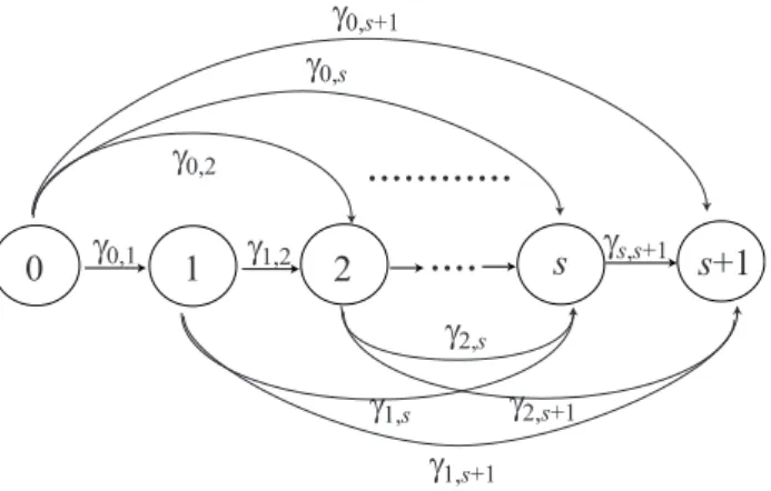
Figure 1: Markovian transition diagram of software degradation level
learning algorithm to the availability model with multi-stage service degradation level. We take place simulation experiments to investigate asymptotic properties of estimators of the optimal software rejuvenation policies maximizing the steady-state system availability. Also we carry out the sensitivity of the turning parameter on the optimal software rejuvenation schedule as a condition-based preventive maintenance policy for a software system.
2. Model Description
Consider an operational software system which may deteriorate with time. State of the software system deteriorates stochastically and changes from i to j (i, j = 0,· · · , s + 1; i < j), where states 0 and s + 1 are the normal (robust) state and the system down state, respectively. Suppose that the state of software at time t, {N(t), t ≥ 0}, is described by a right-skip free CTMC with state space I ={0, 1, · · · , s+1} and that the transition rate from i to j is given by γi,j (> 0), where
∑s+1
j=i+1γi,j = Γi for all i (= 0, 1,· · · , s) (see Figure 1). More precisely, let us define the probability matrix T (t) whose (i, j)-entry is given by
Ti,j(t) = Pr{N(t) = j | N(0) = i}. (2.1)
From the familiar Markovian argument, we have the following Kolmogorov forward equation: d dtT (t) = T (t)Q, (2.2) where Q = −∑γ1,· γ1,2 · · · γ1,s+1 0 −∑γ2,· · · · γ2,s+1 .. . ... . .. ... 0 · · · −γs,s+1 γs,s+1 . (2.3)
Solving the matrix differential equation in Equation (2.2) with the initial condition T (0) = I (identity matrix), the transition probability matrix T (t) can be represented by T (t) = exp{Qt}.
When a system failure occurs, the system is down (j = s + 1) and the recovery operation immediately starts, where the time to complete the recovery operation is an independent and identically distributed (i.i.d.) random variable having the cumulative distribution function (c.d.f.) Hf(x) and mean 1/χ (> 0). On the other hand, one makes a decision whether
to trigger the software rejuvenation or not at the time instant when the state of software system changes from i to j (= i + 1, i + 2,· · · , s). We call this timing decision point. If one decides to continue operation, then the state is monitored until the next change of state, say, decision point, otherwise, the software rejuvenation is preventively triggered, where the time to complete the rejuvenation is also an i.i.d. random variable with the c.d.f. Hr(x) and mean 1/ω (> 0).
It should be noted that the system state N (t) can be described by only the index j (0 ≤ j ≤ s + 1). At each decision point when the state changes from i to j, more specifically, one has an option to choose Action 1 (rejuvenation) or Action 2 (continuation of processing). When the system failure occurs, i.e. the state of system becomes j = s + 1, the recovery operation (Action 3) is taken. Let qi,j(δ) denote the probability that the state changes from i to j under Action δ (= 1, 2, 3) at an arbitrary state. Then, it can be seen that
(i) Case 1 (rejuvenation): qi,0(1) =
∫ ∞ 0
dHr(t) = 1, i = 0, 1,· · · , s, (2.4) where the mean rejuvenation time (overhead) is given by
hr = ∫ ∞
0
tdHr(t). (2.5)
(ii) Case 2 (continuation of processing):
qi,j(2) = γi,j/Γi, i, j = 0, 1,· · · , s + 1, i < j.
(2.6) (iii) Case 3 (recovery from failure):
qi,0(3) = ∫ ∞
0
dHf(t) = 1, (2.7)
where the mean recovery time (overhead) is given by hf =
∫ ∞ 0
tdHf(t). (2.8)
After completing rejuvenation or recovery operation, the state of software system becomes as good as new, i.e., i→ 0 in Equations (2.4) and (2.7), and the same cycle repeats again and again over an infinite time horizon. We define the time interval from the initial operation time (i.e., t = 0) to the completion of rejuvenation or recovery operation whichever occurs first, as one cycle.
3. Semi-Markov Decision Process
Observing the state of software system, we sequentially determine the optimal timing to trigger the software rejuvenation so as to maximize the steady-state system availability, or equivalently to minimize the steady-state system unavailability, which is the probability that the software system is not operative in the steady state. Define the following notation:
δ(i): action taken at state (decision point) i δ(i) = 1 : 0 ≤ i ≤ s 2 : 0 ≤ i ≤ s 3 : i = s + 1. (3.1)
G(i, δ(i)): mean down time between successive decision points, when action δ(i) is taken at state i G(i, δ(i)) = hr : δ(i) = 1 0 : δ(i) = 2 hf : δ(i) = 3. (3.2)
πi(δ(i)): expected total time between successive decision points, when action δ(i) is taken at state i πi(δ(i)) = hr : δ(i) = 1 1/Γi : δ(i) = 2 hf : δ(i) = 3. (3.3)
U (i): action space at state i, i.e., δ(i)∈ U(i).
v(i): relative value function in the semi-Markov decision process at state i∈ I. z∞: steady-state system unavailability, where z∗∞ denotes the minimum one.
From the preliminary above, the Bellman equation based on the principle of optimality is given by v(i) = min δ∈U(i) { G(i, δ)− z∞πi(δ) + s+1 ∑ j=0 qi,j(δ)v(j) } , (3.4)
where the relative value function v(i) means the minimized mean down time provided that the optimal action was continuously taken in the future. It is well known that the software rejuvenation schedule satisfying Equation (3.4) is the best policy among all the Markovian policies [42]. To solve the above functional equation numerically, we can easily develop the well-known value iteration algorithm and policy iteration algorithm for the semi-Markov decision process. Define:
w(i, δ(i)): relative value function when action δ(i) is taken at state i, A(n): = mini∈I{vn(i)− vn−1(i)},
B(n): = maxi∈I{vn(i)− vn−1(i)},
ϵ: tolerance level for iterative calculation,
τ : design parameter in the value iteration algorithm which satisfies 0 ≤ τ/hr ≤ 1, 0 ≤ τ Γi ≤ 1 and 0 ≤ τ/hf ≤ 1 for all i (see [42]),
where wn(i, δ(i)) and vn(i) denote the n-th iterations of the relative value functions and their minimum ones. Then the value iteration algorithm for the Bellman equation in Equa-tion (3.4) is given in the following:
Value Iteration Algorithm: Step 1: n := 0, v0(i) := 0.
Step 2: wn+1(i, 2) := s+1 ∑ j=0 τ γi,jvn(j) + ( 1− s+1 ∑ j=0 τ γi,j ) vn(i), wn+1(i, 1) := hr hr + ( τ hr ) vn(0) + ( 1− τ hr ) vn(i), vn+1(i) := min{wn+1(i, 1), wn+1(i, 2)},
vn+1(s + 1) := hf hf + ( τ hf ) vn(0) + ( 1− τ hf ) vn(s + 1).
Step 3: If 0 ≤ B(n) − A(n) ≤ ϵA(n), then stop the procedure, otherwise, n := n + 1 and go to Step 2.
Also, the policy iteration algorithm for the Bellman equation in Equation (3.4) is given in the following:
Policy Iteration Algorithm:
Step 1: n := 0. Select an arbitrary policy δn.
Step 2: Solve the following linear equations. Any one of the vn terms should be set to 0.
vn(i) = G(i, δn(i))− zn∞πi(δn(i)) + s+1 ∑ j=0
qi,j(δ(i))vn(j).
Step 3: Choose a new policy δn+1 such that
δn+1(i) = argmina∈U(i)´ { G(i, a)− zn∞πi(δn(i)) + s+1 ∑ j=0 qi,j(a)vn(j) } .
Step 3: If the new policy is identical to the old one, that is, if δn+1(i) = δn(i) for each i then stop the procedure, otherwise, n := n + 1 and go to Step 2.
In general, it would be possible to derive numerically the optimal software rejuvenation schedule by applying either value iteration algorithm or policy iteration algorithm, if there exists a unique optimal solution, even though the underlying state process is given by a semi-Markov decision process. It is worth noting, however, that an analytical approach to characterize the optimal rejuvenation policy, without solving the Bellman equation directly, is possible by making some parametric (but reasonable) assumptions. In the following section, we investigate some mathematical properties for the optimal software rejuvenation schedule and prove its optimality.
4. Optimal Software Rejuvenation Policy
In this section, we prove the optimality of the control-limit type of policy, i.e., it is optimal to trigger the software rejuvenation at the first time when the state of software reaches to a pre-specified level, say, N (> 0). We make the following assumptions:
(A-1) Γi is monotonically increasing in i (= 0, 1,· · · , s + 1). (A-2) For an arbitrary increasing function fj,
∑s+1
j=i+1γi,jfj/Γi is monotonically increasing in i (= 0, 1,· · · , j − 1).
(A-3) For an arbitrary x, Hf(x) > Hr(x), where in general H(·) = 1 − H(·).
The assumption (A-1) implies that the mean sojourn time in each state decreases as the system tends to deteriorate. The assumption (A-2) seems to be somewhat technical, but is intuitively reasonable. For instance, let fj be any cost parameter depending on state j. In this case, the mean down time incurred when the system state makes a transition, ∑s+1
j=i+1fj(γi,j/Γi), tends to increase as the degraded level i progresses. In the assumption (A-3), one expects that the recovery time from system failure is strictly greater than the rejuvenation overhead in the sense of probability.
Then, we obtain the following results.
Lemma 4.1. The function v(i) is increasing in i. Proof. It is evident from (A-3) to show that
w(s, 1) = hr+ v(0)− zhr, (4.1)
v(s + 1) = hf + v(0)− zhf. (4.2)
Hence we have v(s) ≤ v(s + 1) immediately. Supposing that v(i + 1) ≤ v(i + 2) ≤ · · · ≤ v(s)≤ v(s + 1) for an arbitrary i, from (A-2), it can be seen that
∑ j γi,j Γi v(j)≤∑ j γi+1,j Γi+1 v(j). (4.3)
In Case 1 with δ(i + 1) = 1, we have
v(i + 1)− v(i) ≥ (hr− hr)− z(hr− hr) = 0. (4.4) This implies that v(i + 1)≥ v(i). In Case 2 with δ(i + 1) = 2, we obtain
v(i + 1)− v(i) ≥ ∑ j γi+1,j Γi+1 v(j)− z/Γi+1− ∑ j γi,j Γi v(j) + z/Γi = ∑ j γi+1,j Γi+1 v(j)−∑ j γi,j Γi v(j) + (z/Γi− z/Γi+1)≥ 0, (4.5)
which is due to (A-1) and (A-2). Thus, it can be shown that v(i) ≤ v(i + 1). From the inductive argument, it can be proved that v(i)≤ v(i + 1) for an arbitrary i.
Theorem 4.1. There exists the optimal control limit N∗+ 1 satisfying
δ(i) = { 1 : otherwise 2 : i≤ N∗. (4.6) Proof. w(i, 2)− w(i, 1) = ∑ j γi,j Γi v(j)− z/Γi− hr− v(0) + zhr. (4.7)
From (A-1) and (A-2) and Lemma 4.1, it is seen that Equation (4.7) is a monotonically increasing function of i. Hence, the proof is completed.
The above theorem is similar to that for the expected cost model in Eto and Dohi [12]. From Theorem 4.1, the problem can be reduced to obtain the optimal control-limit N∗+ 1 so as to minimize the steady-state system unavailability. In fact, this type of rejuvenation policy is essentially the same as the workload-based rejuvenation policy in the transaction-based software system (see e.g. [34]). In other words, even for our non-queueing system framework, the control-limit type of rejuvenation policy is always better than any time-based one.
Next, we formulate the steady-state system unavailability as a function of N , i.e. z∞ = z∞(N ). Define the following functions:
Ri,j = 1 i = j, j ∑ k=i+1 γi,kRk,j/Γi otherwise, (4.8) Si = N ∑ j=i Ri,j/Γj i≤ N, 0 i > N, (4.9)
where Ri,j is the transition probability from state i to state j, and Si denotes the mean time to trigger software rejuvenation at state i. Using the above notation, we can get the following result immediately.
Theorem 4.2. The optimal software rejuvenation time is given by the first passage time (random variable) T∗ = inf{t ≥ 0 : N(t) ≥ N∗+ 1}, where the optimal threshold level N∗ is the solution of z∞∗ = min0≤N<∞z∞(N ):
z∞(N ) = N ∑ j=1 R0,j Γj { s ∑ k=N +1 γj,khk+ γj,s+1hf } S0+ N ∑ j=1 s ∑ k=N +1 R0,j Γj {γj,khr+ γj,s+1hf} . (4.10)
In Equation (4.10), the function z∞(N ) is formulated as the expected down time for one cycle divided by the mean time length of one cycle. The minimization problem of z∞(N ) with respect to N (= 0, 1, 2,· · · ) is trivial. Define the difference of z∞(N ) by ϕ(N ) = z∞(N + 1)− z∞(N ). If ϕ(N + 1)− ϕ(N) > 0, then the function z∞(N ) is strictly convex in N . Further, if ϕ(N∗ − 1) > 0 and ϕ(N∗) ≤ 0, then there exist (at least one, at most two) optimal threshold level N∗ which minimizes z∞(N ). In fact, the convex property of the function z∞(N ) can be easily checked numerically, although we omit to show it.
If the state of software, N (t), is described by SMPs with general transition probability, it is worth noting that Theorem 4.2 is still valid by replacing the transition rate γi,j by γi,j(t). In other words, if one can know the transition probabilities completely, it is possible to obtain the analytical form of the steady-state system unavailability and to minimize it with respect to the threshold level N . However, in such a situation, the control-limit policy is not always guaranteed to be optimal. In the following section, we consider the case where the complete information on the state transition (system deterioration and failure times) is not available. If the underlying state process, N (t), is given by a CTMC, the standard statistical method for estimating the transition rate, like the maximum likelihood estimation, would be applicable. On the other hand, if one can not know whether N (t) follows the CTMC
response ENVIRONMENT
LEARNING AGENT action
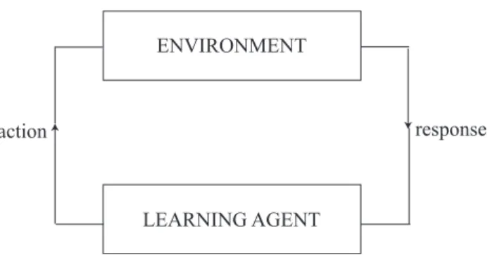
Figure 2: Configuration of reinforcement learning algorithm
in advance, any non-parametric approach has to be used to estimate the optimal software rejuvenation schedule. In the following section, we introduce the reinforcement learning algorithm to estimate the optimal software rejuvenation schedule in an adaptive way. 5. Reinforcement Learning Algorithm
The reinforcement learning is a simulation-based optimization algorithm, where the optimal value function is approximated with the sample or simulation of observations. In general, the reinforcement learning scheme consists of (i) an environment, (ii) a learning agent with its knowledge base, (iii) a set of actions taken by the agent and (iv) responses from the environment to the different actions in different states (see Figure 2). That is, the agent learns an interaction from the environment based on try-and error principle, and adapts the environment itself. The agent can receive the information called reward from the environ-ment, and can learn the parameters which govern the environment. Here, we consider two representative reinforcement learning algorithms, called Q learning and Q-P learning [5], which correspond to the value iteration and policy iteration algorithms, respectively, and define the following three factors:
Observation of state: Observe the current state,
Selection of actions: Select the best action from possible ones at the current state, where the best action is taken based on an estimate of reward (Q value),
Learning from environment: Update Q value with both the current Q value and the reward earned by the selected action.
The Q learning is discussed more specifically within the framework of Markov and/or semi-Markov decision processes. Abounadi et al. [1] improves the classical Q learning algo-rithm and show that it can converge to the optimal relative value function in the dynamic programming equation almost surely. Borkar and Meyn [7] and Konda and Borkar [21] prove some convergence properties on the Q learning-based algorithms with the the ordinary dif-ferential equation (O.D.E.) method and the martingale convergence theorem, respectively. Mahadevan [24] pays his attention to the numerical calculation in the Q learning. For good surveys on the Q learning algorithms in Markov/semi-Markov decision processes, see [5, 17].
Define the following notation:
Q(i, δ(i)): estimate of future cumulative system down time just after the action δ(i) is taken in state i,
P (i, δ(i)): replication of Q(i, δ(i)),
r(i, δ(i), j): system down time until the state transition to j occurs just after the action δ(i) is taken in state i,
REW ARD∞: cumulative system down time in the steady state, provided that an agent selects the action δ(i) with probability 1/|U(i)| so as to minimize the Q value,
T IM E∞: cumulative operation time in the steady state, provided that an agent selects the action δ(i) with probability 1/|U(i)| so as to minimize the Q value,
REW ARDt: cumulative system down time at each decision point, T IM Et: cumulative operation time at each decision point,
ϕ: design parameter in the Q learning algorithm, k, E: number of iterations,
zt: transient (instantaneous) system unavailability, i.e.,
zt = REW ARDt/T IM Et, (5.1)
where limt→∞zt= z∞.
We derive the Q-factor version of the value iteration algorithm mentioned in Section 3. In the first phase of Q learning algorithm (Step 1∼ Step 5 below), the learning agent learns the Q value as an estimate of future cumulative system down time based on a probabilistic action, and adapts the environment through the update of Q value. In the second phase (Step 6 ∼ Step 9 below), the decision maker (DM) regards the first phase as a simulator, and selects the optimal action based on the updated Q value by the agent. Although the DM’s action at each decision point does not influence the agent and the environment, he or she can behave optimally in the sense of minimization of the Q value, and can estimate the updated Q value, say, estimates of the cumulative system down time and cumulative total operation time from the history. The estimates in this stage is transient, i.e., they can function to check the convergence.
Q Learning Algorithm:
Step 1: Agent observes the current state i of software system. Set
k = 0, ϕ = 1, REW ARD∞ = 0, T IM E∞= 0, REW ARDt = 0 and T IM Et= 0. Step 2: For a sufficient large iteration number kz, if k ≤ kz at each observation point with
state i (= 1, 2,· · · , s), then the agent uses a probabilistic strategy, i.e., takes an action δ(i) (rejuvenation (Action 1) or continuation of process (Action 2)) with probability 1/|U(i)|. Further, if the action taken by the agent minimizes Q value, then ϕ = 0, otherwise ϕ = 1. On the other hand, if k ≥ kz, then the agent takes the optimal action which minimizes Q value and stop the procedure.
Step 3: After observing the transition from state i to j, the agent updates the Q value with the probabilistic strategy δ according to the following formula:
Q(i, δ) ←− (1 − α)Q(i, δ) + α {
r(i, δ, j)− z∞t(i, δ, j) + min ´ δ′∈U(j)
Q(j, δ′) }
, where α∈ (0, 1] is the learning rate (constant).
Step 4: If ϕ = 0, then update REW ARD∞ and T IM E∞ as shown below: REW ARD∞ ← REW ARD∞+ r(i, δ, j),
Step 5: Update the minimum steady-state system unavailability z∞ by z∞ ← REW ARD∞/T IM E∞.
Step 6: The DM selects the optimal action at state i, minimizing the Q value updated by δ(i) = argminδ(i)∈U(i)´ Q(i, δ(i)).
Step 7: Update REW ARDt and T IM Et by
REW ARDt← REW ARDt+ r(i, δ(i), j), T IM Et← T IMEt+ t(i, δ(i), j). Step 8: Update zt by
zt← REW ARDt/T IM Et. Step 9: Set k = k + 1 and i← j, and go to Step 2.
In actual implementation of the above algorithm, it should be noted that the action whether to trigger the software rejuvenation or not at each decision point is taken in Step 6. Then, an estimate of the steady-state unavailability is equivalent to that estimated by the learning agent in Step 5 and is independent of the DM’s action. On the other hand, when z∞≈ zt at the maximum iteration number kz, then one can check that the Q learning algo-rithm converges and as the result the maximum steady-state system availability is achieved in the software operation with rejuvenation.
Next, we derive the Q-factor version of the policy iteration algorithm mentioned in Section 3.
Q-P Learning Algorithm:
Step 1: Agent observes the current state i of software system. Set
k = 0, E = 1, ϕ = 1, REW ARD∞ = 0, T IM E∞= 0, REW ARDt = 0 and T IM Et= 0, and initialize P (i, δ(i)) for all state i and all δ(i) to random values.
Step 2: For a sufficient large iteration number kz, if k ≤ kz at each observation point with state i (= 1, 2,· · · , s), then the agent uses a probabilistic strategy, i.e., takes an action δ(i) (rejuvenation (1) or continuation of process (2)) with probability 1/|U(i)|. Further, if the action taken by the agent minimizes Q value, then ϕ = 0, otherwise ϕ = 1. On the other hand, if k≥ kz, then go to Step 10.
Step 3: After observing the transition from state i to j, the agent updates the Q value with the probabilistic strategy δ according to the following formula:
Q(i, δ) ←− (1 − α)Q(i, δ) +α
{
r(i, δ, j)− z∞t(i, δ, j) + Q(j, arg min ´ δ′∈U(j)
P (j, δ′)) }
,
Step 4: If ϕ = 0, then update REW ARD∞ and T IM E∞ as shown below: REW ARD∞ ← REW ARD∞+ r(i, δ, j),
T IM E∞ ← T IME∞+ t(i, δ, j).
Step 5: Update the minimum steady-state system unavailability z∞ by z∞ ← REW ARD∞/T IM E∞.
Step 6: The DM selects the optimal action at state i, minimizing the Q value updated by δ(i) = argminδ(i)∈U(i)´ Q(i, δ(i)).
Step 7: Update REW ARDt and T IM Et by
REW ARDt← REW ARDt+ r(i, δ(i), j), T IM Et← T IMEt+ t(i, δ(i), j). Step 8: Update zt by
zt← REW ARDt/T IM Et. Step 9: Set k = k + 1 and i← j, and go to Step 2.
Step 10: For a sufficient large iteration number Ez, if E ≤ Ez, then set P (i, δ(i)) ← Q(i, δ(i)) and Q(i, δ(i)) = 0 for all i and all δ(i) and go to Step 11. On the other hand, if E ≥ Ez, then the agent takes the optimal action which minimizes Q value and stop the procedure.
Step 11: Set k = 0, E ← E + 1, and go to Step 2.
In the following section, we give an illustrative examples and investigate the convergence properties of the Q learning algorithm and Q-P learning algorithm.
6. Numerical Examples 6.1. CTMC case
First, we consider the case where the temporal dynamics of software state is given by a right-skip CTMC, and derive the optimal software rejuvenation schedule when the statistical information on the state transition is completely known. Huang et al. [20], Dohi et al. [9] suppose that the number of system states is only 3: normal operation, deterioration (failure probable state) and system down (failure). Here, we consider a more generalized Markovian deterioration process with 3 degradation levels (totally, 5 states), where the associated infinitesimal generator is given by
Q = −0.1 0.04 0.03 0.02 0.01 0 − 0.1 0.04 0.04 0.02 0 0 −0.1 0.06 0.04 0 0 0 −0.1 0.1 .
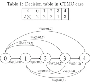
In this case we have ω = 0.4 and χ = 0.2. In Table 1, we obtain the so-called decision table to characterize the optimal software rejuvenation schedule. From this result, it is optimal to trigger the software rejuvenation at the first time when the system state reaches to i = N∗+ 1 = 3. Then the associated minimum unavailability is given by z∗∞ = z∞(2) = 0.038041.
Table 1: Decision table in CTMC case i 0 1 2 3 4 δ(i) 2 2 2 1 3 1 0 exp(0.04) 2 3 4 exp(0.04) exp(0.04) exp(0.04) Wei(0.03,2) Wei(0.02,2) Wei(0.01,2) Wei(0.02,2) Wei(0.06,2) Wei(0.1,2)
Figure 3: An example with three degradation levels
6.2. SMP case
Next, we consider more general case where the state transition is governed by a semi Markov process (SMP). For better understanding the situation, we do not use the notation of tran-sition rate γi,j(t), but instead of the following one:
exp(λ): exponential distribution with mean 1/λ,
W ei(η, m): Weibull distribution with scale parameter η and shape parameter m
for notational simplicity. Figure 3 depicts the SMP with respective transition probabilities, where ω = 0.4 and χ = 0.2 similar to the CTMC case. Table 2 presents the decision table for the SMP case, where the optimal threshold is given by N∗ = 1 and the corresponding steady-state system unavailability is z∗∞ = 0.04028. As mentioned before, the resulting rejuvenation schedule may not be strictly optimal. However, if we pay our attention to only the control-limit policy, this is of course optimal to maximize the steady-state system availability.
6.3. On-line adaptive rejuvenation scheduling
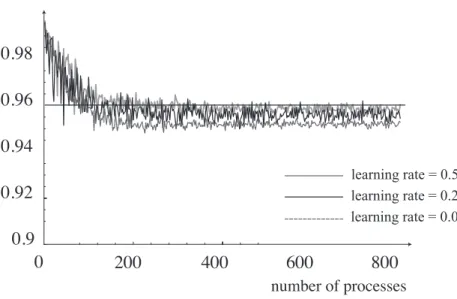
Of our concern is the investigation of convergence properties of the Q learning and Q-P learning algorithms. We perform the Monte Carlo simulation with pseudo random numbers for the exponential and the Weibull distributions with the same parameters in Subsec-tion 6.2, and observe the realizaSubsec-tions of state deterioraSubsec-tion time and system failure time. At each decision (observation) point, we behave so as to minimize the Q value and estimate both z∞ and zt. Hereafter, we fix the upper limit of iteration number as kz = 10000 in Q learning algorithm case. Also, we fix the iteration numbers as kz = 100 and Ez = 100 in Q-P learning algorithm case. Figures 4 and 5 show the asymptotic behavior of estimates of the steady-state system availability for varying learning rate; 0.01, 0.20, 0.50, in Q learning algorithm and Q-P learning algorithm respectively, where the horizontal line denotes the real maximized value, 1− z∗∞ = 0.95972. In these figures, we define the unit of a process as the time length of one cycle. From these figures, it is seen that estimates of the steady-state system availability asymptotically converges to the real optimal solution 1−z∗ = 0.95972 as
Table 2: Decision table in SMP case i 0 1 2 3 4 δ(i) 2 2 1 1 3 0.9 0.92 0.94 0.96 0.98
steady-state system availability
200 400 600 800 number of processes 0 learning rate = 0.20 learning rate = 0.01 learning rate = 0.50
Figure 4: Asymptotic behavior of steady-state system availability based on Q learning for varying learning rate
the number of processes increases. Note again that this can be achieved with the probabilis-tic action by the agent. In Q learning case, if the learning rate is given by 0.10 and 0.50 when the number of processes is fixed as 200, the relative error with respect to 1− z∗∞= 0.95972 becomes 0.31% and 0.86%, respectively. Also, in Q-P learning case, if the learning rate is given by 0.10 and 0.50 when the number of processes is fixed as 200, the relative error with respect to 1− z∗∞ = 0.95972 becomes 0.33% and 0.51%, respectively.
In general, though the smaller learning rate leads to much more computation, it does not always guarantee the smaller error.For instance, when the number of processes is 800 when the learning rate is given by 0.01, the relative errors become 0.14% in Q learning case, and 0.13% in Q-P learning case, respectively. That is, the careful adjustment of the learning rate would be important to realize the effective estimation by taking account of computational effort. In Table 3, we calculate the estimation errors (%) between estimate and the real optimal solution with high accuracy, where|z∗∞−z∞|/(1 − z∗∞). As the learning rate decreases, the estimation error decreases and afterward the Q learning and Q-P learning tend to estimate the steady-state system availability.
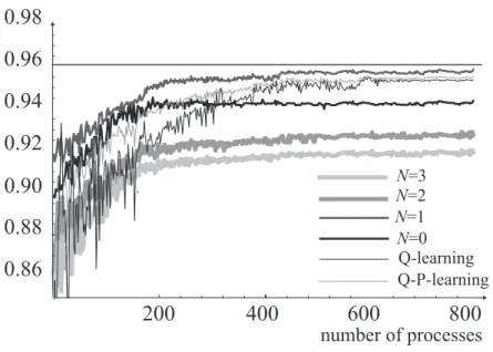
Next, we examine the asymptotic behavior of the transient system availability based on the DM’s action. For the example in the previous SMP case, if the complete information on the system deterioration/failure time distributions is available, one can know that the optimal threshold level is given by N∗ = 1 and would continue applying the control-limit policy with N∗ = 1. Then, our main concern is to examine the performance of the Q learning and Q-P learning characterized by choosing the minimum Q value. That is, if the estimate of transient system unavailability, zt, is closed to the real optimal solution, z∗∞, it can be concluded that the resulting Q learning and Q-P learning can provide the similar
0.9 0.92 0.94 0.96 0.98
steady-state system availability
200 400 600 800 number of processes 0 learning rate = 0.20 learning rate = 0.01 learning rate = 0.50
Figure 5: Asymptotic behavior of steady-state system availability based on Q-P learning for varying learning rate
Table 3: Dependence of learning rate on estimation of steady-state system availability with Q learning and Q-P learning
number of processes Q -learning Q -P -learning learning rate 200 400 800 200 400 800 0.01 0.31% 0.04% 0.14% 0.33% 0.25% 0.13% 0.05 0.15% 0.02% 0.15% 0.34% 0.31% 0.15% 0.10 0.04% 0.05% 0.19% 0.39% 0.34% 0.15% 0.20 0.33% 0.30% 0.27% 0.40% 0.37% 0.18% 0.30 0.63% 0.30% 0.32% 0.42% 0.39% 0.22% 0.40 0.73% 0.53% 0.47% 0.45% 0.44% 0.26% 0.50 0.86% 0.85% 0.70% 0.51% 0.49% 0.32%
transient system availability Q-learning N=2 N=1 N=0
200
400
600
800
number of processes N=3 Q-P-learning0.86
0.88
0.92
0.94
0.96
0.98
0.90
Figure 6: Comparison of Q-learning and Q-P -learning policies with some control-limit ones in simulation
effect on system availability to the best (but unknown) control limit policy. In Figure 6, we carry out the simulation and compare the Q learning and Q-P learning algorithms with the rejuvenation schedule with fixed threshold level N (= 0, 1, 2, 3). In the same parametric circumstance as Table 3, we plot the behavior of estimates of 1− zt. In this simulation experiment, since it is shown analytically that N∗ = 1 is optimal, it can be easily expected that the simulation result with N∗ = 1 approaches to 1−z∗∞= 0.95972. On the other hand, the rejuvenation schedule based on the Q learning and Q-P learning give the fluctuated results in earlier phase, and latter converge to the real optimal as the number of processes increases, respectively. Additionally, we derive a result that Q-P learning converges at an early age in comparison with Q learning, but both of two algorithms share its asymptotic characteristic. It is evident that the simulation-based algorithm used here can never outper-form the really optimal rejuvenation policy, say, N∗ = 1. However, in the situation where no statistical information on the system deterioration/failure time distributions is available, this non-parametric estimation scheme would be useful.
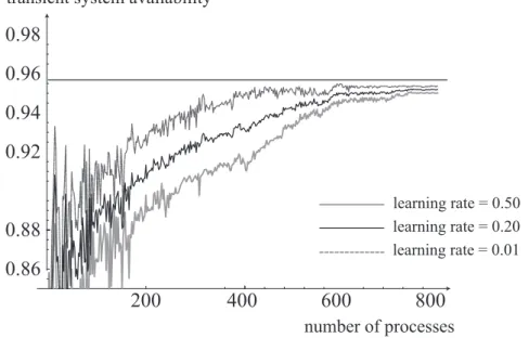
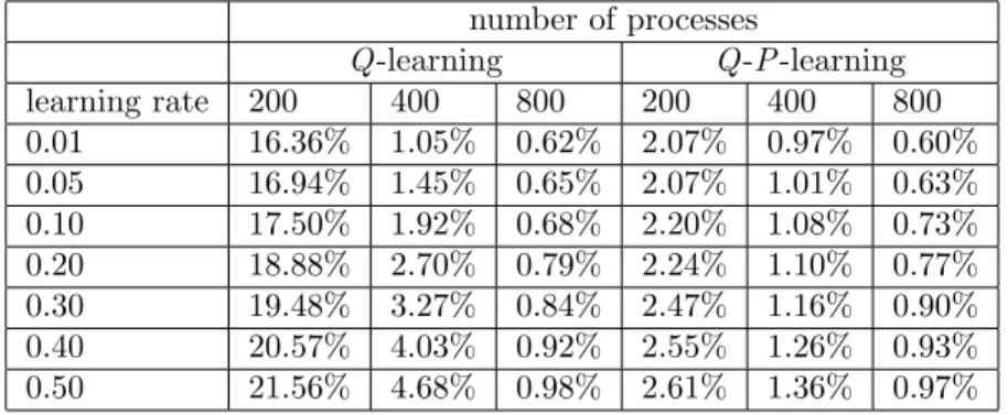
Figures 7 and 8 illustrate the dependence of learning rate on the transient system avail-ability 1−ztat arbitrary time t in Q learning case and Q-P learning case respectively, where the estimate of system availability with smaller learning rate approaches to the steady-state availability 1− z∞ as the number of processes increases. In Table 4, we calculate the esti-mation errors (%) between estimates of transient availability and the real optimal with high accuracy, where |z∗∞− zt|/(1 − z∗∞). As the learning rate decreases, the estimation error decreases and afterward the Q learning and Q-P learning tend to estimate the steady-state availability.
7. Conclusions
In this paper we have considered an operational software system with multi-stage degrada-tion levels due to software aging, and derived the optimal dynamic software rejuvenadegrada-tion
0.86 0.88 0.92 0.94 0.96 0.98
transient system availability
200 400 600 800
number of processes
learning rate = 0.20 learning rate = 0.01 learning rate = 0.50
Figure 7: Asymptotic behavior of transient system availability based on Q learning for varying learning rate
0.86 0.88 0.92 0.94 0.96 0.98
transient system availability
200 400 600 800 number of processes learning rate = 0.20 learning rate = 0.01 learning rate = 0.50 0.90
Figure 8: Asymptotic behavior of transient system availability based on Q-P learning for varying learning rate
Table 4: Relative error of estimates of transient system availability to the steady-state one number of processes Q -learning Q -P -learning learning rate 200 400 800 200 400 800 0.01 16.36% 1.05% 0.62% 2.07% 0.97% 0.60% 0.05 16.94% 1.45% 0.65% 2.07% 1.01% 0.63% 0.10 17.50% 1.92% 0.68% 2.20% 1.08% 0.73% 0.20 18.88% 2.70% 0.79% 2.24% 1.10% 0.77% 0.30 19.48% 3.27% 0.84% 2.47% 1.16% 0.90% 0.40 20.57% 4.03% 0.92% 2.55% 1.26% 0.93% 0.50 21.56% 4.68% 0.98% 2.61% 1.36% 0.97%
policy maximizing the steady-state system availability, via the semi-Markov decision process. In addition, we have developed a reinforcement learning algorithm as an on-line adaptive nonparametric estimation scheme without the knowledge of transition rate to each degra-dation level. In simulation experiments, we have investigated the asymptotic behavior of estimates of the optimal software rejuvenation policy with the reinforcement learning. The Q-learning-based algorithms have rich convergence properties to the unknown optimal solu-tions as the number of data increases. At the same time, it is known that the computation is rather expensive and the convergence speed is relatively slow. In the future work, we plan to implement the resulting Q-learning algorithms on a real software system and to conduct an experiment to examine the feasibility of our on-line adaptive software rejuvenation scheme. References
[1] J. Abounadi, D. Bertsekas, and V.S. Borkar: Learning algorithms for Markov decision processes with average cost. SIAM Journal on Control and Optimization, 40 (2001), 681–698.
[2] E. Adams: Optimizing preventive service of the software products. IBM Journal of Research & Development, 28 (1984), 2–14.
[3] J. Alonso, R. Matias Jr., E. Vicente, A. Maria, and K.S. Trivedi: A comparative experimental study of software rejuvenation overhead. Performance Evaluation, 70 (2013), 231–250.
[4] Y. Bao, X. Sun, and K.S. Trivedi: A workload-based analysis of software aging, and rejuvenation. IEEE Transactions on Reliability, 54 (2005), 541–548.
[5] D.P. Bertsekas and N.J. Tsitsiklis: Neuro-Dynamic Programming (Athena Scientific, 2001).
[6] A. Bobbio, M. Sereno, and C. Anglano: Fine grained software degradation models for optimal rejuvenation policies. Performance Evaluation, 46 (2001), 45–62.
[7] V.S. Borkar and S.P. Meyn: The O.D.E. method for convergence of stochastic approx-imation and reinforcement learning. SIAM Journal on Control and Optimization, 38 (2000), 447–469.
[8] V. Castelli, R.E. Harper, P. Heidelberger, S.W. Hunter, K.S. Trivedi, K.V. Vaidyanathan, and W.P. Zeggert: Proactive management of software aging. IBM Jour-nal of Research & Development, 45 (2001), 311–332.
[9] T. Dohi, K. Goseva-Popstojanova, and K. S. Trivedi: Estimating software rejuvenation schedule in high assurance systems. The Computer Journal, 44 (2001), 473–485.
[10] T. Dohi, H. Okamura, and K.S. Trivedi: Optimizing software rejuvenation policies under interval reliability criteria. Proceedings of The 9th IEEE International Conference on Autonomic and Trusted Computing (ATC-2012), (IEEE CPS, 2012), 478–485. [11] T. Dohi, H. Okamura, and K.S. Trivedi: Optimal periodic software rejuvenation policies
based on interval reliability criteria. under submission.
[12] H. Eto and T. Dohi: Optimality of control-limit type of software rejuvenation policy. Proceedings of The IEEE 11th International Conference on Parallel and Distributed Systems (ICPADS-2005), II (IEEE CPS, 2005), 483–487.
[13] H. Eto and T. Dohi: Analysis of a service degradation model with preventive rejuvena-tion. In D. Penkler, M. Reitenspiess and F. Tam (eds.): Service Availability: Third In-ternational Service Availability Symposium (ISAS-2006), LNCS 4328 (Springer-Verlag, 2006), 17–29.
[14] H. Eto and T. Dohi: Determining the optimal software rejuvenation schedule via semi-Markov decision process. Journal of Computer Science, 2 (2006), 528–534.
[15] H. Eto, T. Dohi, and J. Ma: Simulation-based optimization approach for software cost model with rejuvenation. In C. Rong, M.G. Jaatun, F.E. Sandnes, L.T. Yang, and J. Ma (eds.): The 5th International Conference on Autonomic and Trusted Computing (ATC-2008), LNCS 5060 (Springer-Verlag, 2008), 206–218.
[16] S. Garg, S. Pfening, A. Puliafito, M. Telek, and K.S. Trivedi: Analysis of preventive maintenance in transactions based software systems. IEEE Transactions on Computers, 47 (1998), 96–107.
[17] A. Gosavi: Simulation-based Optimization: Parametric Optimization Techniques and Reinforcement Learning (Kluwer Academic Publishers, 2003).
[18] J. Gray: Why do computers stop and what can be done about it? Proceedings of The 5th International Symposium on Reliable Distributed Software and Database Systems, (IEEE CPS, 1986), 3–12.
[19] M. Grottke and K.S. Trivedi: Fighting bugs: Remove, retry, replicate, and rejuvenate. IEEE Computer, 40 (2007), 107–109.
[20] Y. Huang, C. Kintala, N. Koletti, and N.D. Fulton: Software rejuvenation: Analysis, module and applications. Proceedings of The 25th International Symposium on Fault Tolerant Computing (FTCS-1995), (IEEE CPS, 1995), 381–390.
[21] V.R. Konda and V.S. Borkar: Actor-critic-type learning algorithms for Markov decision processes. SIAM Journal on Control and Optimization, 38 (1999), 94–123.
[22] F. Machida, D.S. Kim, and K.S. Trivedi: Modeling and analysis of software rejuvenation in a server virtualized system with live VM migration. Performance Evaluation, 70 (2013), 212–230.
[23] F. Machida, V.F. Nicola, and K.S. Trivedi: Job completion time on a virtualized server with software rejuvenation. ACM Journal on Emerging Technologies in Computing Systems, 10 (2014), 10–26.
[24] S. Mahadevan: Average reward reinforcement learning: Foundations, algorithms for Markov decision processes. SIAM Journal on Control and Optimization, 38 (2000), 94–123.
[25] T. Nakagawa: Maintenance Theory of Reliability (Springer-Verlag, 2005).
[26] H. Okamura and T. Dohi: Application of reinforcement learning to software rejuvena-tion. Proceedings of The 10th International Symposium on Autonomous Decentralized Systems (ISADS-2011) (IEEE CPS, 2011), 647–652.
[27] H. Okamura and T. Dohi: Dynamic software rejuvenation policies in a transaction-based system under Markovian arrival processes. Performance Evaluation, 70 (2013), 197–211.
[28] H. Okamura, T. Dohi, and K.S. Trivedi: On-line adaptive algorithms in autonomic restart control. In B. Xie, J. Branke, S.M. Sadjadi, D. Zhang and X. Zhou (eds.): The 7th International Conference on Autonomic and Trusted Computing (ATC-2010), LNCS 6407 (Springer-Verlag, 2010), 32–46.
[29] H. Okamura, H. Fujio, and T. Dohi: Fine-grained shock models to rejuvenate software systems. IEICE Transactions on Information and Systems (D), E86-D (2003), 2165– 2171.
[30] H. Okamura, J. Guan, C. Luo, and T. Dohi: Quantifying resiliency of virtualized sys-tem with software rejuvenation. IEICE Transactions on Fundamentals of Electronics, Communications and Computer Sciences (A), E98-A (2015), 2051–2059.
[31] H. Okamura, S. Miyahara, and T. Dohi: Dependability analysis of a client/server software systems with rejuvenation. Proceedings of The 13th International Symposium on Software Reliability Engineering (ISSRE-2002), (IEEE CPS, 2002), 171–180. [32] H. Okamura, S. Miyahara, and T. Dohi: Dependability analysis of a transaction-based
multi server system with rejuvenation. IEICE Transactions on Fundamentals of Elec-tronics, Communications and Computer Sciences (A), E86-A (2003), 2081–2090. [33] H. Okamura, S. Miyahara, and T. Dohi: Rejuvenating communication network system
with burst arrival. IEICE Transactions on Communications (B), E88-B (2005), 4498– 4506.
[34] H. Okamura, S. Miyahara, T. Dohi, and S. Osaki: Performance evaluation of workload-based software rejuvenation scheme. IEICE Transactions on Information and Systems (D), E84-D (2001), 1368–1375.
[35] H. Okamura, K. Yamamoto, and T. Dohi: Transient analysis of software rejuvenation policies in virtualized system: Phase-type expansion approach. Quality Technology and Quantitative Management Journal, 11 (2014), 335–352.
[36] S. Pfening, S. Garg, A. Puliafito, M. Telek, and K.S. Trivedi: Optimal rejuvenation for tolerating soft failure. Performance Evaluation, 27/28 (1996), 491–506.
[37] K. Rinsaka and T. Dohi: Behavioral analysis of fault-tolerant software systems with rejuvenation. IEICE Transactions on Information and Systems (D), E88-D (2005), 2681–2690.
[38] K. Rinsaka and T. Dohi: Non-parametric predictive inference of preventive rejuvenation schedule in operational software systems. Proceedings of The 18th International Sympo-sium on Software Reliability Engineering (ISSRE-2007), (IEEE CPS, 2007), 247–256. [39] K. Rinsaka and T. Dohi: Estimating the optimal software rejuvenation schedule with
small sample data. Quality Technology and Quantitative Management Journal, 6 (2009), 55–65.
[40] K. Rinsaka and T. Dohi: Toward high assurance software systems with adaptive fault management. Software Quality Journal, 24 (2016), 65–85.
[41] R.S. Sutton and A. Barto: Reinforcement Learning (MIT Press, 1998).
[42] H.C. Tijms: Stochastic Models: An Algorithmic Approach (John Wiley & Sons, 1994). [43] K.V. Vaidyanathan and K.S. Trivedi: A comprehensive model for software rejuvenation.
[44] A.P.A. van Moorsel and K. Wolter: Analysis of restart mechanisms in software systems. IEEE Transactions on Software Engineering, 32 (2006), 547–558.
[45] D. Wang, W. Xie, and K.S. Trivedi: Performability analysis of clustered systems with rejuvenation under varying workload. Performance Evaluation, 64 (2007), 247–265. [46] C. Watkins and P. Dayan: Q-learning. Machine Learning, 8 (1992), 279–292.
[47] W. Xie, Y. Hong, and K.S. Trivedi: Analysis of a two-level software rejuvenation policy. Reliability Engineering and System Safety, 87 (2005), 13–22.
[48] W. Yurcik and D. Doss: Achieving fault-tolerant software with rejuvenation and re-configuration. IEEE Software, 18 (2001), 48–52.
[49] J. Zhao, Y.B. Wang, G.R. Nin, K.S. Trivedi, R. Matias Jr., and K.-Y.Cai: A compre-hensive approach to optimal software rejuvenation. Performance Evaluation, 70 (2013), 917–933.
Tadashi Dohi
Department of Information Engineering Hiroshima University
1–4–1 Kagamiyama, Higashi-Hiroshima 739-8527, Japan