2008, Vol. 51, No. 1, 1-14
HEURISTIC FOR BALANCING U-SHAPED ASSEMBLY LINES WITH PARALLEL STATIONS
Sihua Chen Louis Plebani
Aristocrat Technologies, Inc. Lehigh University (Received March 22, 2005; Revised May 17, 2006)
Abstract This paper presents a version of the U-shaped Assembly Line Balancing Problem and an asso-ciated heuristic solver where parallel stations are used to accommodate tasks with processing time greater than the cycle time. Computational results for the heuristic applied to problems created from industry standard test sets show that the heuristic performs well when compared to optimum solution bounds.
Keywords: Algorithm, heuristic, assembly line balancing
1. Introduction
Assembly line configurations are one of most ubiquitous and important aspects in manufac-turing. The Assembly Line Balancing Problem (ALBP) is to group tasks into workstations such that the sum of the processing times at each station does not exceed a station uni-form cycle time. The precedence constraints on the tasks are typically shown by an acyclic graph such as Figure 1. The digits outside the nodes represent the constant processing
3 6 7 4 4 6 5 4 5 3 6 7 11 1 5 2 6 8 10 3 4 7 9 12 4 6
Figure 1: Example of a precedence network
times for the corresponding tasks. The assembly tasks cannot be sub-divided and must be completed at their assigned work-station. There are two common versions of this problem: the minimization of the number of workstations for a given cycle time (SALBP-I) and the minimization of the cycle time for a given number of workstations (SALBP-II) which is typically attacked by repetitively solving SALBP-I problems. Figure 2 shows an optimal SALBP-I straight line solution for the example of Figure 1 and a cycle time of 10 time units. Seven workstations are needed.
The advent of just-in-time (JIT) manufacturing has driven industries to search for man-ufacturing methodologies with lean concepts and high efficiency in both inventory and labor. Largely due to pressures of JIT, many assembly lines are now being designed as U-shaped
Station 2 Station 3 Station 4 Station 5 Station 6 Station 1 Station 7 4 2 5 3 6 4 4 5 6 6 4 7 3 8 7 1 5 9 7 10 3 11 6 12 Cycle Time = 10
Figure 2: Straight assembly line solution to Figure 1
assembly lines [16]. In addition to the potential for better balancing, they typically have im-proved visibility and communications, fewer work stations, more flexibility for adjustment, minimization of operation travel, and easier material handling when compared to straight lines. Figure 3 shows an optimal U-shaped assembly line for the example network of Fig-ure 1. Only six workstations are required as compared to the seven workstations required in the straight assembly line case.
4 2 6 4 4 5 6 6 4 7 3 8 1 5 9 7 10 3 11 6 12 5 3 Station 4 Station 5
Station 1 Station 2 Station 3 Station 6
7
Cycle Time = 10
Figure 3: U-shaped assembly line solution to Figure 1
Since the ALBP was first introduced by Salveson in 1955 [21], numerous researchers have investigated straight line assembly line balancing [9]. Freeman and Jucker [8] introduced parallel workstations into the straight line problem. Buxey [5] studied the practical aspects of parallel stations and noted that the costs of duplicated equipment and difficulties of layout and transportation detracted from the essential benefits of just-in-time flow line production in most cases. He concluded that parallel stations should be tightly constrained and only be used to accommodate tasks with time larger than the line cycle time. If no tasks exceed the cycle time, no parallel stations should be used.
The study of U-shaped assembly line balancing has been much more limited. The first published work on U-shaped lines was in 1994 [15]. For the same reasons as those of the straight assembly line, the successful application of U-shaped assembly lines depends upon efficient line balancing. Yet, only a limited body of research has been reported in the area of U-shaped line balancing [1, 7, 11, 14, 15, 17–19, 23]. A major reason for the sparseness of reported research is the fact that both assembly line balancing and sequencing are known to be NP-Hard problems [6, 9, 24].
To date, no detailed research has been reported on U-shaped assembly line balancing with parallel stations, although Boysen and Fliedner [4] suggest that their two-stage graph algorithm could be adapted to the problem. This paper presents a version of the U-shaped assembly line balancing problem which allows parallel stations to be used on a U-shaped line. It incorporates a constraint implementing Buxey’s conclusion that parallel stations should only be used when necessary to accommodate a task whose time is larger than the line cycle
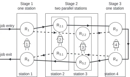
R1 R6 R3 R4 Stage 1 one station Stage 2 two parallel stations
Stage 3 one station R2.1 R5.1 job entry job exit R2.2 R5.2 1 2 3 4
station 1 station 2 station 3 station 4
Figure 4: U-line showing task sets and work flow
time. This type of line is applicable to JIT production environments where labor cost is relatively high and it is common to use smaller and inexpensive equipment [16]. Section 2 presents a mathematical model of the problem. Section 3 describes a heuristic solver for this problem. Section 4 summarizes the computational results of the heuristic applied to problems created from industry standard test sets. Section 5 is concluding remarks. The appendix in Section 6 presents a worked example.
2. Mathematical Model
A U-shaped assembly line with parallel stations can be viewed as a traditional U-shaped line where stations are replaced with stages. A stage may contain two or more identical workstations operating in parallel. We define the following variables:
T : {i : i = 1 . . . N} the set of all tasks to be assigned.
ti : the processing time of task i
P : the set of task pairs indicating task precedence. For all {x, y} ∈ P , task x must be completed before task y begins.
C : the line cycle, the pace of production.
qk : the number of identical workstations in stage k.
M : the number of stages.
Rk : for k = 1,2,..M, the set of tasks that are processed at the stage k
during the first half of the U-line;
R2M +1−k : for k = 1, 2, ..M , the set of tasks that are processed at the stage k
during the second half of the U-line;
Sk : the set of all tasks processed in stage k.
The sets R are identified in the schematic of a 3 stage U-shaped line, with 2 parallel stations in the second stage shown in Figure 4. Assume a cycle time of 6 minutes and that the sum of task times is represented by R1 = 3, R2 = 4, R3 = 4, R4 = 2, R5 = 8, and R6 = 3,
where R5 consists of a single indivisible task. Since R5 = 8, the parallel stations as shown
in the figure are necessary to obtain the desired cycle time. The processing is as follows. Operator 1 works on station R1 for 3 min(work forward) and turns to work on R6 for 3
min(work backward). Operator 2 works on station R2.1 for 4 min(work forward) and turns
to work on R5.1 for 8 min(work backward). Operator 3 works on station R2.2 for 4 min(work
forward) and turns to work on R5.2 for 8 min(work backward). Operator 4 works on station R3 for 4 min(work forward) and turns to work on R4 for 2 min(work backward).
The objective of the mathematic model is to minimize the total idle time in the system M X k=1 qkC − N X i=1 ti (2.1)
which is equivalent to minimizing the total number of stations. A complete model is: Minimize M X k=1 qk (2.2) Subject to: Sk = Rk∪ R2M +1−k, k = 1, 2, .., M (2.3) M [ k=1 Sk = T (2.4) Si∩ Sj = ∅, for all i 6= j (2.5) X i∈Sk ti ≤ qkC, k = 1, 2, .., M (2.6)
for all (x, y) ∈ P : if x ∈ Ri and y ∈ Rj, then i ≤ j (2.7)
qk = » t∗ k C ¼ , where t∗k = max i∈Sk ti (2.8)
Equations (2.3) define the tasks assigned to each stage. Equation (2.4) ensures that all the tasks are assigned. Equations (2.5) ensure that each task is assigned to only one stage. Inequalities (2.6) limit the total workload in a stage to the capacity of that stage. Con-ditions (2.7) enforce the precedence restrictions. Equations (2.8) enforce Buxey’s practical constraint that, in a high tech assembly environment, parallel stations should only be used when necessary to accommodate a task time which exceeds the cycle time.
3. Heuristic for U-line with Parallel Stations
Heuristic solution approaches for the straight line and non-parallel U-line ALBP have in-cluded priority rule based procedures [12], simulated annealing [26], tabu search [20], and genetic algorithms [10]. While exact methods using Integer Programming, Dynamic Pro-gramming and particularly Branch and Bound [2, 9, 22] have had some success with small to modest size problems, heuristic procedures are needed for larger problems, for finding initial feasible solutions and bounds for exact methods, and for use in solving variations of the ALBP using search procedures where the SALBP-I problem is repetitively solved. The HUP (Heuristic for U-shaped Parallel lines) heuristic is offered as a solver for the present problem. HUP always returns a feasible solution.
The HUP heuristic is based upon Hackman’s [12] IUFF heuristic for straight assembly line balancing which in turn was based upon Wee and Magazine’s [27] GFF heuristic for straight lines. In a manner similar to these heuristics, HUP balances the line by scoring, ranking, and assigning tasks to workstation stages until all tasks are assigned.
Talbot, et.al. [25] compiled a list of the numerical scoring functions that have been used by Hackman [12], Wee and Magazine [27], and other researchers in constructing decision rules for assembly line balancing heuristics. Four of these are meaningful for the parallel station U-shaped line problem. Each of these rules assigns a score reflecting the importance of a task in terms of some measure such as time or number of tasks that they “control” with respect to assignment of tasks to workstations. The HUP heuristic uses all four with appropriate U-line adaptations. They are:
• Work element time (WE): the processing time of a task. The largest WE has the highest
priority.
• Positional weight (PW): If the task is eligible for assignment in the forward direction (no
unassigned predecessors) then PW is the sum of unassigned task times that follow it. If the task is eligible for assignment in the backward direction (no unassigned successors) then PW is the sum of unassigned task times that precede it. The largest PW has the highest priority.
• Number of followers (NF) : If the task is eligible for assignment in the forward direction
(no unassigned predecessors) then NF is the number of unassigned tasks that follow it. If the task is eligible for assignment in the backward direction (no unassigned successors) then NF is the number of unassigned tasks that precede it. The largest NF has the highest priority.
• Number of immediate followers (NIF) : If the task is eligible for assignment in the forward
direction (no unassigned predecessors) then NIF is the number of unassigned tasks that immediately it. If the task is eligible for assignment in the backward direction (no unassigned successors) then NIF is the number of unassigned tasks that immediately precede it. The largest NIF has the highest priority.
In addition to the modifications necessary to accommodate U-shaped lines and parallel sta-tions, HUP improves over earlier heuristics by immediately adjusting scores and re-ranking available tasks after each task assignment. The adjustment and re-ranking is important for U-lines since the assignment of tasks to either end of the line can immediately affect ranking scores in the case of PW, NIF, and NF criteria.
Preliminary investigation determined that it was not possible to predict which of the four scoring function would provide the best solution (smallest number of stations) for any particular network. Because of this, we decided to investigate whether a new scoring function that combined the other four would provide value to the heuristic. Because of the incompatibility of the units of measure reported by the other scoring functions, the new function combines the rank returned by the other functions rather than the raw values. The new ranking function is called scored rank of scores (SRS) and is calculated as follows:
1. the tasks are ranked with each of the 4 ranking functions;
2. for each task, the ordinal rank corresponding to each function is summed;
3. the resulting sums are sorted to determine the SRS ranking. Lowest value has highest priority.
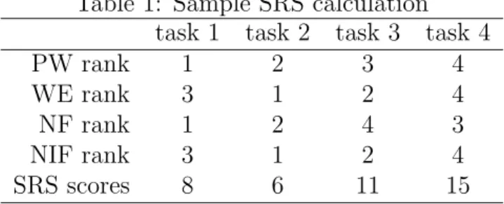
Table 1 illustrates SRS applied to four tasks. The first four lines show the ranking for the tasks corresponding to each of the ranking functions. The SRS line is the sum of ranked scores. Ranking this line would order the tasks {t2, t1, t3, t4}, where t2would highest priority
for assignment. When SRS was incorporated into HUP, it too resulted in a better solution for some problems than the other scoring functions.
Table 1: Sample SRS calculation task 1 task 2 task 3 task 4
PW rank 1 2 3 4
WE rank 3 1 2 4
NF rank 1 2 4 3
NIF rank 3 1 2 4
Start HUP
For all Scoring rules WE, PW, NF,NIF, SRS Allocate all tasks Done all 5 Select best of 5 assignments Done
Allocate all tasks
Create New Stage Add available tasks to A No Yes Yes No Select ( i) highest ranked
task from A. Buxey allow expansion? Yes No No C ti£ Assign task to stage A empty? Yes all allocated? Add parallel stations to stage No slack ti< Return No Yes Yes
Assign task to Stage
Adjust slack time
Adjust ranking scores for tasks
in A Return 0 = slack Yes No
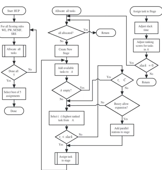
Figure 5: HUP heuristic
Because each of the scoring rules has occasions to yield a better solution than the re-maining rules, and because HUP executes quickly, HUP’s default strategy is to determine an assignment using each of the five scoring functions separately and then to choose the best of the resulting five solutions. HUP uses the following variables:
slack : slack time for a station in the current stage;
A : set of tasks available for assignment because they currently have either no predecessors or no successors;
n : stage number;
qn : number of parallel stations in the current stage;
qtest : temporary value for number of stations n the current stage used
to test if stage can be expanded;
ri : ranking score for task i;
ti : time for task i;
ttest : temporary time value used to test if stage can be expanded
A flowchart of HUP is shown in Figure 5. For a given scoring rule, the following steps allocate tasks to stages:
Step 1: Close any open stage. Create a new stage (n = n + 1, qn = 1, A = ∅, slack = C, )
Step 2: Add all tasks having no unassigned predecessors and/or no unassigned successors to A. For each task added to A, calculate the associated ranking score.
Step 3: If A = ∅, go to Step 1. Otherwise, select and remove the highest ranking task i from
A.
If ti ≤ slack assign task i to the current stage. Go to Step 5.
If slack < ti ≤ C, the task cannot be assigned to the current stage. Go to Step 3.
If ti > C, the task can be added to the current stage if the stage can be expanded with
parallel stations. Go to Step 4.
Step 4: If the current stage has already been expanded, the Buxey constraint on minimizing duplicated equipment does not allow further expansion. The task cannot be assigned. Go to Step 3.
If the time consumed by tasks already assigned to an unexpanded station require the stage to be expanded beyond the minimum size necessary to accommodate the current large task, expansion would also violate the Buxey constraint. To check this, calculate:
qtest= » ti C ¼ (3.1)
ttest = slack + (qtest− 1)C (3.2)
If the ti ≤ ttest, then the stage can be expanded. Expand the station and add the task
(qn= qtest, slack = ttest− ti). Then Go to Step 5.
If the stage cannot be expanded go to Step 3.
Step 5: For scoring functions other than WE, appropriately adjust the ranking scores for the tasks remaining in A which have the current task i as a predecessor or successor. If
slack = 0, go to Step 1, otherwise go to Step 2.
4. Computational Results
The HUP heuristic was coded in C++ and run on a 733Mhz Pentium computer. The test suite of problems was constructed from the benchmark data sets of Talbot, Patterson & Gehrlein [25], Hoffman [13], and Scholl & Klein [23]. These data sets have been used for testing and comparing solution procedures for assembly line balancing problems in almost all relevant studies since the early nineties. As the present problem is a new version of the ALBP, there are no existing exact solvers or heuristic solvers for it other than the present HUP algorithm. In order to evaluate the heuristic three comparisons were made. The first was based upon known optimal solutions to U-line non-parallel problems. The second used lower bounds to U-line parallel problems. The third compared the HUP heuristic to a straight line with parallel stations heuristic that also incorporated the Buxey constraint.
In order to obtain a base line for evaluation, the number of workstations as determined by HUP was compared with published solutions to non-parallel U-line problems based on the benchmark networks. There are 269 problems in this test set. The 269 problems took a total of 3.75 seconds or 0.014 seconds per problem to execute. The results are summarized in Table 2. The well known bin-packing lower bound for ALBP’s, LB = dPt/Ce is also
included in the table. In the table, deviation and relative deviation of the solution s from
x is defined as s − x and (s − x)/x, respectively. “Optimal” in the table refers to the
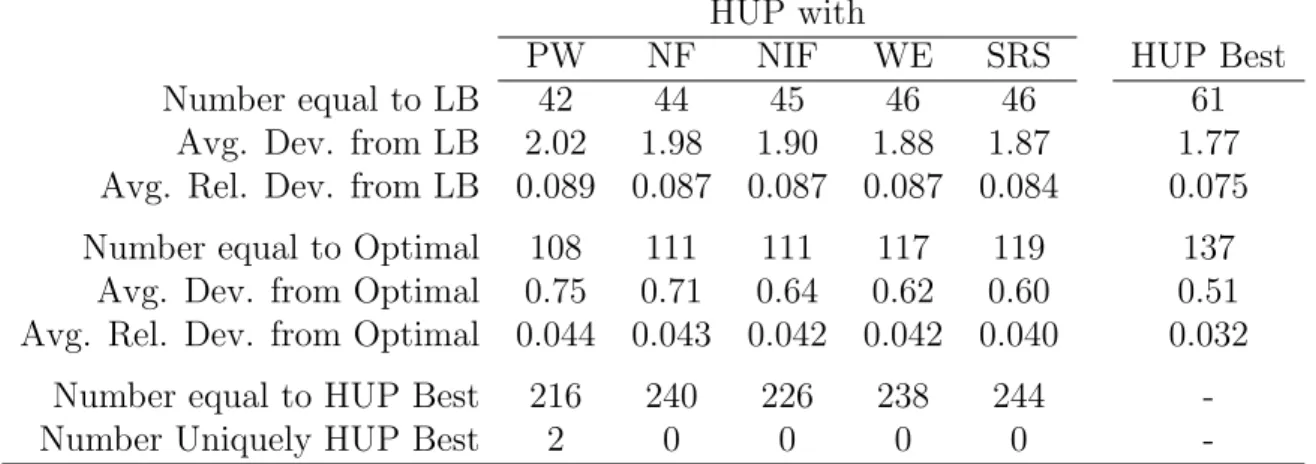
known optimal solution for a test problem. “HUP Best” refers to the best solution, i.e., the smallest number of stations, found with HUP and the five scoring rules. “Uniquely HUP Best” indicates a situation using HUP where the respective scoring rule was the only rule of the five to achieve the best solution. Table 2 shows that HUP found the optimal solution for 137 of the 269 problem instances.
Table 2: Summary for 269 U-line non-parallel problems HUP with
PW NF NIF WE SRS HUP Best
Number equal to LB 42 44 45 46 46 61
Avg. Dev. from LB 2.02 1.98 1.90 1.88 1.87 1.77 Avg. Rel. Dev. from LB 0.089 0.087 0.087 0.087 0.084 0.075
Number equal to Optimal 108 111 111 117 119 137
Avg. Dev. from Optimal 0.75 0.71 0.64 0.62 0.60 0.51 Avg. Rel. Dev. from Optimal 0.044 0.043 0.042 0.042 0.040 0.032
Number equal to HUP Best 216 240 226 238 244
-Number Uniquely HUP Best 2 0 0 0 0
-HUP was then used to solve a set of problems each of which required at least one stage of two or more parallel stations. These problems were formed by varying the cycle time for each of the benchmark networks from the minimum task time to one less than the maximum task time of the respective network. There were a total of 14829 problems in this test set. The problems took 311 seconds or an average time of 0.021 seconds per problem to run. The longest problem took 0.33 seconds. This corresponded to the somewhat unrealistic case where the largest network of 297 tasks was run with a very small cycle time resulting in nearly 14000 parallel stations. When the smallest cycle time was limited to 80% of the largest task time, the average time per problem was 0.011 seconds with the longest problem time of 0.08 seconds. The results for the parallel problems are summarized in Table 3.
Table 3: Summary for 14829 U-line parallel problems HUP with
PW NF NIF WE SRS HUP Best
Number equal to LB 1494 1678 2378 2173 2334 3219 Avg. Dev. from LB 7.10 6.93 6.76 6.67 6.67 6.32 Avg. Rel. Dev. from LB 0.069 0.065 0.062 0.062 0.061 0.054 Number equal to HUP Best 6971 8237 10023 10786 10440
-Number Uniquely HUP Best 102 232 713 1364 626
-It is clear that the HUP heuristic found the optimal solution to at least 21.7% of the 14829 parallel test problem cases, i.e., for those cases for which the HUP solution was equal to the lower bound LB. This correlates favorably with the non-parallel case (refer to Table 2) where the heuristic had 22.6% of its solutions equal to LB. For these non-parallel problems the optimal solution was found nearly 51% of the time. The average deviation from LB of the HUP solutions is larger for the parallel solutions than for the non-parallel case because of the large number of stations resulting from small values of cycle time. The average relative deviations attempt to normalize the effect of large solution values. The average relative deviations from LB are actually much better than in the non-parallel case. If one accepts the hypothesis that the smaller average relative deviations of the parallel case implies the relationship between an LB solution and an optimal solution for the parallel case is at least as good as the non-parallel case, it can be concluded that HUP finds the optimal solution on average 50+% of the time.
Table 4: Straight line parallel results HUP with
PW NF NIF WE SRS HUP Best
Number equal to LB 851 442 872 553 783 1071
Avg. Dev. from LB 8.01 8.79 7.93 8.56 8.15 7.62 Avg. Rel. Dev. from LB 0.085 0.101 0.085 0.096 0.088 0.078 Number inferior to U-line 8210 12278 9348 12191 11007 10727
Avg. additional stations 1.72 2.56 1.61 2.20 2.00 1.80
The test set of problems was also used to compare the solutions for the U-line with parallel stations problems with the solutions for a straight line when parallel stations are allowed within the context of the Buxey constraint. The HUP heuristic was modified for straight line solution by only considering tasks feasible for assignment to a station if the tasks had no predecessors. The resulting straight line heuristic was used to solve the 14829 parallel problems in the test set. Table 4 compares the straight line parallel solutions to the U-line parallel solutions. The first three lines of the table provide statistics from the comparison of the straight line solutions to the lower bounds. The fourth line counts the number of problems for which the straight line solution had at least one more station than the U-line solution for the same problem. The last line is the average number of additional stations required by the inferior straight line solutions. Comparison of the U-line to straight line solutions affirms the superiority of the U-line configuration in that fewer stations were required in over 72% of the problems solved.
5. Summary
This paper presented a version of the assembly line balancing problem that uses U-shaped lines where parallel stations are permitted if and only if they are necessary to achieve a desired cycle time. The HUP heuristic was provided as a solver for this problem and was shown to execute quickly. By extrapolating results from known solutions to non parallel problems, it was estimated that the HUP heuristic has an approximate 50% success rate in obtaining optimal solutions.
6. Appendix: Worked Example
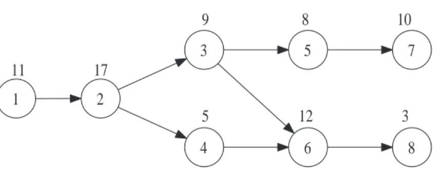
1 2 7 8 5 6 3 4 9 8 10 5 12 3 17 11
Figure 6: Example problem precedence diagram
The following lists the steps of the HUP algorithm as applied to Bowman’s network shown in Figure 6. Positional weight (PW) will be used for the scoring function. The cycle time of 10 will be used.
Step 1: Create a new station.
n = 1, q1 = 1, A = ∅, slack = 10
Step 2: Compute ranking scores for available tasks and add tasks to A.
r1 = 11 + 17 + 9 + 5 + 8 + 12 + 10 + 3 = 75 r7 = 10 + 8 + 9 + 17 + 11 = 55
r8 = 3 + 12 + 9 + 5 + 17 + 11 = 57 A = {1, 8, 7}
Steps 3 & 4: Highest ranking task in A (task 1) has t1 > C. Since this is the first task added
to this stage, expansion definitely possible. Expand the stage and assign task 1.
q1 = §t 1 C ¨ =§11 10 ¨ = 2 slack = q1C − t1 = 20 − 11 = 9 A = {8, 7}
Step 5: Since task 1 is no longer part of their positional weight, adjust rankings scores (PW in this case) of tasks in A having task 1 as a predecessor by subtracting t1.
r7 ← r7− t1 = 55 − 11 = 44 r8 ← r8− t1 = 57 − 11 = 46
Go to Step 2
Step 2: Task 2 now has no predecessors. Calculate ranking score and add task 2 to A.
r2 = 17 + 9 + 5 + 8 + 12 + 10 + 3 = 64 A = {2, 8, 7}
Step 3: Highest ranking task in A (task 2) has t2 > C, Go to Step 4.
Step 4: Stage 1 has already been expanded. Task 2 cannot be added.
A = {8, 7}
Go to Step 3
Step 3: Highest ranking task is task 8. Since t8 ≤ slack, assign to stage 1. slack ← slack − t8 = 9 − 3 = 6
A = {7}
Go to Step 5
Step 5: Task 7 does not have task 8 as a predecessor or successor. No adjustments necessary. Go to Step 2.
Step 2: Compute ranking scores for newly available tasks and add tasks to A.
r6 = 12 + 9 + 5 + 17 = 43 A = {7, 6}
Step 3: All available task times are greater than slack. Go to Step 1. Step 1: Close stage 1 = {1, 8} with 2 parallel stations. Open new stage.
n = 2, q2 = 1, A = ∅, slack = 10
Step 2: Add available tasks to A. Compute ranking scores as required.
r2 = 17 + 9 + 5 + 8 + 12 + 10 = 61 r7 = 44, r6 = 43, A = {2, 7, 6}
Steps 3 & 4: Task 2 the highest ranking task in A has t2 > C. Since this is the first task added
to this stage, expansion definitely possible. Expand the stage and assign task 2.
q2 = §t 2 C ¨ =§17 10 ¨ = 2 slack = q2C − t2 = 2 · 10 − 17 = 3
Go to Step 5
Step 5: Adjust scores of tasks in A having task 2 as a predecessor.
r6 ← r6− t2 = 43 − 17 = 26 r7 ← r7− t2 = 44 − 17 = 27
Go to Step 2
Step 2: Add newly available tasks to A and compute ranking scores.
r3 = 9 + 8 + 12 + 10 = 39 r4 = 5 + 12 = 17
A = {3, 7, 6, 4}
Step 3: Times of all tasks in A are greater than slack. Go to Step 1. Step 1: Close stage 2 = {2} with 2 parallel stations. Open new stage.
n = 3, q3 = 1, A = ∅, slack = 10
Step 2: Add available tasks to A. Compute ranking scores as required.
r3 = 39, r7 = 27, r6 = 26, r4 = 17 A = {3, 7, 6, 4}
Steps 3 & 5: Highest ranking task in A is task 3. Since t3 ≤ slack, assign task 3 to stage 3.
Adjust scores of tasks in A having task 3 as a predecessor.
slack ← slack − t3 = 1 r6 ← r6− t3 = 17 r7 ← r7− t3 = 18
Go to Step 2
Step 2: Add newly available tasks to A and compute ranking scores. Ties in task rankings will be broken by task time.
r5 = 8 + 10 = 18 A = {7, 5, 6, 4}
Step 3: Times of all tasks in A are greater than slack. Go to Step 1. Step 1: Close stage 3 = {1} with 1 station. Open new stage.
n = 4, q4 = 1, A = ∅, slack = 10
Step 2: Add available tasks to A.
r7 = 18, r5 = 18, r6 = 17, r4 = 17 A = {7, 5, 6, 4}
Step 3 & 5: Task 7 is highest ranking task in A. Since t7 ≤ slack, assign task 7 to stage 3. slack ← slack − t7 = 0
Adjust scores of tasks in A having task 3 as a successor.
r5 = 18 − 10 = 8
Since slack = 0, Go to Step 1
Step 1: Close stage 4 = {7} with 1 station. Open new stage.
n = 4, q5 = 1, A = ∅, slack = 10
Step 2: Add available tasks to A.
r6 = 17, r4 = 17, r5 = 8 A = {6, 4, 5}
Step 3 & 4: Task 6 is highest ranking task in A has t6 > C. Since this is the first task added
q4 = §t 6 C ¨ =§12 10 ¨ = 2 slack = q4C − t6 = 20 − 12 = 8 A = {5, 4}
Step 5: Adjust scores of tasks in A having task 6 as a successor.
r4 ← r4− t6 = 5
Go to Step 2
Steps 2, 3 & 5: No newly available tasks. Task 5 is highest ranking task in A. Since t5 ≤ slack,
assign task 5.
slack ← slack − t5 = 0 A = {4}
r4 ← r4− t6
Since slack = 0, Go to Step 1
Step 1 & 2: Close stage 5 = {5, 6} with 2 stations. Open new stage. There are no new tasks to add.
n = 6, q6 = 1, A = {4} , slack = 10
Step 3: Only task in A is task 4. Since t4 ≤ slack. Assign task 4.
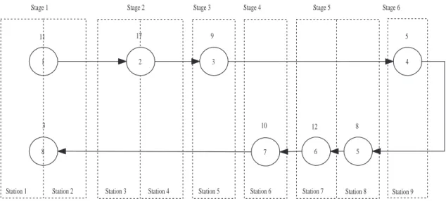
All tasks have been assigned. The HUP solution consisting of 6 stages and 9 stations: is shown in Table 5 and Figure 7.
Table 5: HUP solution for Bowman network with parallel stations Stage (k) Parallel Stations (qk) Tasks (Sk)
1 2 1,8 2 2 2 3 1 3 4 1 7 5 2 5,6 6 1 4 References
[1] D. Ajenblit and R. Wainwright: Applying genetic algorithms to the U-shaped assembly line balancing problem. Proceedings of the IEEE Conference on Evolutionary
Compu-tation (1998), 96–101.
[2] I. Baybars: A survey of exact algorithms for the simple assembly line balancing problem.
Management Science, 32 (1986), 909–932.
[3] E. Bowman: Assembly-line balancing by linear programming. Operations Research, 8 (1960), 385–389.
[4] N. Boysen and M. Fliedner: A versatile algorithm for assembly line balancing. European
Journal of Operational Research, 184 (2008), 39–56.
[5] G. Buxey: Assembly line balancing with multiple stations. Management Science, 20 (1974), 1010–1021.
[6] A. Chakravarty and A. Shtub: Balancing mixed model lines with in-process inventories.
1
8
Station 1 Station 2 Station 5
3 2
Station 6
Station 3 Station 4 Station 7
7 Station 8 6 5 4 Station 9 11 17 9 5 3 10 12 8
Stage 1 Stage 2 Stage 3 Stage 4 Stage 5 Stage 6
Figure 7: HUP solution for Bowman network with parallel stations
[7] W. Chiang, P. Kouvelis, and C. Chen: An efficient heuristic for the U-shaped assem-bly line balancing problem in the just-in-time production environment. Proceedings of
National Annual Meeting to the Decision Sciences (1997), 1126.
[8] J. Freeman and J. Jucker: The line balancing problem. Journal of Industrial
Engineer-ing, 18 (1967), 361–364.
[9] S. Ghosh and R. Gagnon: A comprehensive literature review and analysis of the design, balancing and scheduling of assembly systems. International Journal of Production
Research, 27 (1989), 637–670.
[10] J. Goncalves and J. De Almeida: A hybrid genetic algorithm for assembly line balanc-ing. Journal of Heuristics, 8 (2002), 629–642.
[11] F. Guerriero and J. Miltenburg: The stochastic U-line balancing problem. Naval
Re-search Logistics, 50 (2003), 31–57.
[12] S. Hackman, M. Magazine, and T. Wee: Fast, effective algorithms for simple assembly line balancing problems. Operations Research, 37 (1989), 916–924.
[13] T. Hoffmann: Eureka: a hybrid system for assembly line balancing. Management
Sci-ence, 38 (1992), 39–47.
[14] H. Hwang, J. Sun, and T. Yoon: U-line line balancing with simulated annealing.
Pro-ceedings of the First Asia-Pacific Decision Sciences Institute Conference (Hong Kong,
1996), 101–108.
[15] G. Miltenburg and J. Wijngaard: The U-line balancing problem. Management Science, 40 (1994), 1378–1388.
[16] J. Miltenburg: U-shaped production lines: A review of theory and practice.
Interna-tional Journal of Production Economics, 70 (2001), 201–214.
[17] K. Nakade and K. Ohno: Analysis and optimization of a U-shaped production line.
Journal of Production Research Society of Japan, 40 (1996), 90–104.
[18] K. Nakade and K. Ohno: Stochastic analysis of a U-shaped production line with mul-tiple workers. Computers and Industrial Engineering, 33 (1997), 809–812.
[19] K. Nakade and K. Ohno: An optimal worker allocation problem for a U-shaped pro-duction line. International Journal of Propro-duction Economics, 60 (1999), 353–358.
[20] R. Pastor, C. Andres, A. Duran, and M. Perez: Tabu search algorithms for an industrial multi-product and multi-objective assembly line balancing problem, with reduction of the task dispersion. Journal of the Operational Research Society, 53 (2002), 1317. [21] J. Salveson: The assembly line balancing problem. Journal of Industrial Engineering,
6 (1955), 18–25.
[22] A. Scholl and R. Klein: Balancing assembly lines effectively – A computational com-parison. European Journal of Operational Research, 114 (1999), 50–58.
[23] A. Scholl and R. Klein: ULINO: Optimally balancing U-shaped JIT assembly lines.
International Journal of Production Research, 37 (1999), 721–736.
[24] D. Sparling: Topics in U-line balancing. Ph.D Dissertation, McMaster University (1997).
[25] F. Talbot, J. Patterson, and W. Gehrlein: A comparative evaluation of heuristic line balancing techniques. Management Science, 32 (1986), 430–454.
[26] R. Vilarinho and A. Simaria: A two-stage heuristic for balancing mixed-model assembly lines with parallel stations. International Journal of Production Research, 40 (2002), 1405–1420.
[27] T. Wee and M. Magazine: Assembly line balancing as generalized bin packing.
Opera-tions Research Letters, 1 (1982), 56–58.
Louis Plebani
Industrial and Systems Engineering Lehigh University
200 West Packer Ave. Bethlehem, PA 18015-1582 E-mail: [email protected]