The Optimal (r,S) Policy in a Single Item Production/Inventory System with Setup Times

Journal of the Operations Research Society of Japan

Vol. 38, No. 2, June 1995

THE OPTIMAL (r,S) POLICY IN A SINGLE ITEM PRODUCTION/INVENTORY SYSTEM WITH SETUP TIMES

Hyo-Seong Lee Kyung Hee University

(Received December 7, 1992; Revised April 11, 1994)

Abstract In this paper, the (r,S) policy is considered for production/inventory systems where a single type items are produced on an item by item basis by a single production facility. The (r,S) policy considered in this paper is a pull type threshold policy which is very useful in situations where the time and cost required to setup the production facility are relatively high. The demand for the item is assumed to arrive according to a Poisson process. The processing time required to produce an item is assumed to follow an arbitrary distribution. When an item is demanded, one of the items in the inventory is delivered to the customer and the kanban on the item is removed. The removed kanban is immediately transmitted to the production facility. At the instant r kanbans are accumulated at the production facility, the operator turns the production facility on, which takes a random amount of time. In the production period, items are produced one by one and whenever each item is produced, a kanban is attached to it. When there are no kanbans at the production facility, the machine is shut. off and a non-production period begins, which lasts until the number of kanbans accumulated at the production facility is raised back to r. In this paper, assuming a linear cost structure, an efficient search procedure is developed to find the optimal threshold value r as well as the optimal number of kanbans S, which minimizes the expected cost incurred per unit time.

1. Introduction

Production/Inventory systems can be classified into two types, viz., push and pull types. In push type systems, the amount of demands for an item is forecasted in advance and the production schedule is set based on this forecast value. In pull type systems, on the other hand, production schedule is not set beforehand, but is decided by the evolution of the demand process of the item. This pull type system is actually operated by means of the kanban, a sort of card or tag. Since the successful applications of the pull type systems were reported in Japanese industry, there has been a considerable work in modeling of production/inventory systems within the framework of pull type systems.

It is known that the pull type system works particularly well under the conditions of smoothed demands and reduced setup times. However, even when the setup costs/times are high, the pull type system could be applied successfully in some manufacturing envi-ronments as will be considered in this paper. We consider in this paper a pull type pro-duction/inventory system in which a single production facility produces items of a given type. Items are produced one by one by a single production facility with completed items going directly into output store. The processing time for producing (replenishing) one item is assumed to be an independent, identically distributed, random variable which follows an arbitrary distribution. Each time production is initiated, a random amount of time to turn the facility on is required. We assume that whenever each item is produced, a kanban is attached to it. Thus, to every item in the output store, a kanban is attached. The demand © 1995 The Operations Research Society of Japan

for the item is assumed to arrive according to a Poisson process with rate A. If an item is demanded, one of the items in the output store is delivered to the customer if the inventory is available. At this time, the kanban on the item is removed. When this removed kanban is transmitted to the production facility, it becomes a production authorization card, that is, the presence of one kanban at the production facility authorizes the production of one item. If the inventory is not available at the instant of a demand arrival, the demand is backordered. We assume that there are unlimited raw materials available in front of the production facility at all times.

If the time and cost required to setup the production facility are negligible, we can use the following very simple policy[lJ: produce whenever kanbans are available. However, when the setup cost/time is high, such a policy could be very costly. Thus in this case, to avoid the frequent setup of the machine, the following threshold policy can be adopted:

When an item is demanded, one of the items in the output store is delivered to the customer and the kanban on the item is removed. The removed kanban, which is now activated as a production authorization card, is immediately transmitted to the production facility. When the number of kanbans accumulated at the production facility reaches r while the machine is shut off, the non-production period terminates and the operator takes a random amount of time to turn the production facility on, which initiates the production period. As soon as the setup is completed, items are produced one by one. During the production period as during the non-production period, removed kanbans are transmitted to the production facility whenever the items are delivered to the customers. When there are no kanbans at the production facility, the machine is shut off and a non-production period begins. The non-production period lasts until the number of kanbans accumulated at the production facility is raised back to r, at which moment the non-production period ends and the next production period begins, initiating another cycle.

inventory level

end of beginning end of production of setup setup

one cycle

---~4"

end of production Figure 1. the (r,S) policy for a production/inventory system with setup times

The Optimal (r,S) Policy 143 Suppose that the total number of kanbans, i.e., the maximum inventory level in the output store, is S. Since our policy is specified by values of the two control variables, namely, the total number of kanbans, S, and the threshold value, T', we will call this policy the (T', S) policy in this paper. Notice that the inventory level in the output store at the beginning of the production period is always S - T' and the inventory level at the end of the production period is always S. From this fact it is easily noticed that if we set 8 = S - T', the (T',S) policy in this paper is just the (8,S) policy for the production/inventory system in the literature (see figure 1)

Associated with this (T', S) production/inventory system we impose the following classical cost structure: i) inventory holding costs are incurred linearly over time with respect to the inventory level ii) backorder costs are incurred linearly over time with respect to the backorder level and iii) a set-up cost is incurred each time the production facility is turned on. The objective of this study is to find an optimal (T', S) policy which minimizes the expected cost per unit time in the long run.

The (T', S) policy in this paper is particularly useful in the situations where the production facility is used for some secondary work during a non-production period. For instance, when the production period ends, the production facility is switched to a secondary mode of operation and is used to produce items of another type. The production facility could be used to repair failed items or to rework defective items during the non-production period. In some cases, the regular maintenance work is performed during the non-production period. Since significant startup costs are usually incurred to switch the machine from one operation mode to another, the (T', S) policy would be very effectively used in all these situations. Other applications of the (T', S) policy could be found, for example, in multiproduct scheduling problems or production schedule in the chemical industry (see Gavish and Graves[5]).

Another type of policy which could be used to avoid the frequent setup of the machine is the (8,Q) policy[l]. In the (8,Q) policy, the total number of kanbans is 8

+

Q and the kanbans removed from the items at the instant of demand arrivals are kept in the output store until the number of kanbans reaches Q. 'Whenever Q kanbans are accumulated, they are sent to the production facility immediately. At the production facility, production is performed so long as it has kanbans. When there are no kanbans at the production facility, the machine is shut off and a non-production period begins. The non-production period continues until Q kanbans are transmitted from the output store to the production facility. As soon as the production facility receives Q kanbans, it is setup and the production period begins. Note that the inventory level at the end of each non-production period is always 8 in the (8, Q) policy.

Therefore, in the (8,

Q)

policy, if more than

Q

demands arrive during the production of Q items, the production period does not terminate as soon as the production of these Q items are completed. In this case, since the production facility receives another Q kanbans while producing the first Q items, it produces at least another batch of Q items. Hence the number of items produced in one production period is always a multiple of Q. It should be noticed that the (8, Q) policy is just the traditional production/inventory policy with fixed reproduction point 8 and production quantity Q.,

It appears that the (8, Q) policy is a more planned policy compared to the (T', S) policy in that it has a predetermined production batch size

Q.

However, when the demand rate is very high, it is probable that more than one batches are produced in one production period. This fact indicates that the length of the production period is strongly dependent on the demand process in the (8,Q) policy. In addition, in the (8,Q) policy, since the inventory level at the end of the production period is not fixed, the variation of the length of the non-production period is very high compared to the (T', S) policy. Therefore, the (8, Q) policy is not suitable

for the situations where the non-production period is used for some secondary work. For this reason we analyze in this study only the (r, S) policy.

The operating policy considered in this paper is a kind of the (8, S) policy. The (8, S)

policies are known to be optimal in a variety of inventory situations where as many inventories as needed can be replenished all at once([S], [11]). However, the (r, S) policy considered in this study is different from these (8, S) policies in that the replenishment of the inventory can be done only on an item-by-item basis. Since the replenishment is made on an item-by-item basis, it is easy to note that our model has an analogy with an M/G/1 queueing system. In fact, when the upper control value S is set to zero, our (r, S) policy becomes the Heyman's N-policy[6]. Recently for this special case where the item is not produced to inventory as in job-shop systems, Federgruen and So proved that the (r,O) policy is optimal among all policies under very general assumptions[2].

While much work has been done on

(8,

S) inventory policies, only limited work has been done on (r, S) policies in which inventory is replenished on an item-by-item basis. The first model for this type of production/inventory system was introduced by Tijms [10]. He consid-ers a system with unit POiSSOIl demands, general processing times and general setup times. He finds the optimal control values by using a denumerable state semi-Markov decision process. Gavish and Graves[4] consider a system with Poisson demands and deterministic processing times. In a subsequent paper, Gavish and Graves[5] extend the analysis to consider general processing times. Srinivasan and Lee[9] consider a more general model with compound Pois-son demands, general processing times and with random inspection intervals. They develop an efficient search procedure to find the optimal policy. Federgruen and Zheng[3] consider a similar model with a more general cost structure. In their study, they derive an efficient algorithm for determination of the optimal policy.

The production/inventory model considered in this paper is rather simple compared with Srinivasan and Lee's model or Federgruen and Zheng's model. In their models, however, setup times to turn the production facility on are not considered. Thus properties of the cost functions developed in their studies are not guaranteed to hold for the systems with setup times. Tijms[10] and Gavish and Graves[5] consider models with setup times. However, a semi-Markov decision process approach used by Tijms is reported (Gavish and Graves[4]) to take too much computational time compared to an intelligent search technique. Gavish and Graves use an efficient search procedure to find an optimal policy when setup times do not exist. In this search procedure some properties for cost functions are effectively exploited. But, when setup times exist, such an intelligent search procedure is not presented since no special properties for cost functions are proved in this case.

In this paper, we analyze the same (r, S) inventory system as the one considered by Tijms or Gavish and Graves. However, for the system with setup times, we characterize the cost functions by deriving a set of properties these cost functions possess. Then by exploiting these properties effectively, we develop an extremely efficient search procedure to find an optimal policy.

2. Analysis Let

V(t) = distribution of the setup time,

v,

v(2)

=

mean and the second moment of the setup time,

bj

=

probability that number of demands which arrive during a setup time is j, j

=

0,1,2,··· ,

U(t)

=

distribution of the processing time to produce a unit item, il, u(2)

=

mean and the second moment of the processing time,

The Optimal (r,S) Policy 145

qj

=

probability that number of demands which arrive during one processing time is

j,j=0,1,2,''', K = setup cost

Ch = holding cost/item/unit time, Cb

=

backorder cost/item/unit time,

C(r, S) = sum of expected holding and backorder costs during a cycle when rand S are used as control values,

L( r) = expected length of a cycle when r is used as a control value,

TC(r, S) =: expected cost per unit time when rand S are used as control values.

N ate that we use L( r) instead of L( r, S) to denote the expected cycle time when rand S

are used as control values. This is because the expected cycle time is a function of r alone. For stability of the system, we assume that the production rate is greater than the demand rate, that is, p = All

<

1.

Our first objective in this paper is to obtain an expression for TC(r, S), the expected cost per unit time for given control values rand S. The approach used to obtain an expression for TC(r, S) is based on that used in Srinivasan and Lee [9]. Let the time interval from the beginning epoch of a non-production period to the beginning epoch of the subsequent non-production period be defined as a cycle. Then from the renewal reward theorem [7], the expected cost per unit time when rand S are used as control values, is obtained by (2.1 ) TC( S) _r, = K

+

_{L ( r ) '} C(r,S)

To obtain C(r,S) and L(r), we divide a cycle into the following three sub-periods:

(i) Period 1 begins when the facility is turned off and lasts until the inventory level drops to S - r for the first time.

(ii) Period 2 begins at the end of period 1 (beginning epoch of a setup time) and lasts until the inventory level is raised back to S - r for the first time.

(iii) Period 3 begins at the end of period 2 and lasts until the inventory level reaches S for the first time.

Let Cl(r,S) denote the expected cost incurred during period 1 and C3(r,S) denote the expected cost incurred during period 3. Note that the expected cost incurred during period

2 is completely determined by the inventory leyel at the beginning epoch of period 2. Let

Ck denote the expected cost incurred during period 2 which is initiated with k items in inventory. Then, since the inventory level at the beginning epoch of period 2 when rand S are used as control values is S - r, the expected cost incurred during period 2 is just (~S-r' Therefore, the sum of the expected holding and backorder costs during a cycle is expressed as

(2.2)

We now show how the terms Cl(r, S), C3(r, S) and

CS-

r are obtained.

Computing the term Cl (r, S)

The expected total cost during period 1 is easy to calculate. Let gk,k-l denote the expected cost incurred from the epoch at which the inventory level becomes k to the epoch when the inventory level drops to k - 1 during a non-production period. If k

2::

0, the cost

for carrying k items is incurred until the next demand arrives and if k

<

0, the cost for backlogging -k items is incurred until the next demand arrives. Thus 91<:,1<:-1 is given by

(2.3a) 91<:,1<:-1 =;:k, Ch if k

2::

0,

(2.3b) _ Cbk

A ' if k

<

O.

The expected cost during period 1 when rand S are used as control values is then expressed by (2.4) S C1(r,S) =

E

I<:=S-r+1 91<:,1<:-1'

Computing the term C3(r, S)

During the production period, the production completion epochs are the times at which the inventory is replenished. To compute C3(r, S), we restrict our attention only to these epochs. Let fi,j denote the expected cost from the epoch at which the inventory level reaches i to the epoch at which the inventory level is raised to j(j

2::

i) for the first time with li,i = 0

for any integer i. Then the expected total cost incurred during period 3, C3(r, S), is just

IS-r,s

which, in turn, is expressed as

S-l

(2.5) C3(r,S) =

IS-r,s

=

E

11<:,1<;+1,

I<:=S-r

From equation (2.5), we see that the term C3(r, S) is obtained if we can calculate each value

of hl<;+l.

If we set

illl<: = hl<;+l - 1k-1,1<:, for all k,

/1<:,1<:+1 is computed recursively using the following lemma. The proof of lemma 2.1 is given in the appendix.

Lemma 2.1

The term /1<:,1<:+1 is expressed recursively as

(2.6.a) U 1k,1<:+1 =11<:-1,1<: - (1 _ p) Cb for k ::; 0, 1 1 00 I<: U 00 (2.6.b) /1<:-1,1<:

+

-{illl<:-l

+

~

E

qj(Ch

+

Cb) -

E

qjilll<:_j

+

~Cb

E

qj}, k

>

0, qo j=1<: j=l P j=l<;+l

with an initial value

Cb AU(2) _

1-1,0 = (1 _ p) {2(1 _ p)

+

u},

where p = AU.

The Optimal (r,S) Policy

Let

(2.7) Tk = 9k+l,k

+

!k,k-+1, for all k.

Then, using equations (2.2), (2.4), (2.5) and (2.'1), C(r, S) is expressed as

S-l

(2.8) C(r, S) =

L

Tk

+

CS-To

k=S-r

To compute the term

CS-

r , we need the following lemma.

Lemma 2.2

The term Ck is expressed recursively as (2.9)

00

Ck = Ck-l

+

L

bj(Tk-l -- Tk-l-j), for all k. j=O

147

Proof Let

e"

denote the expected cost incurred during a setup time that is initiated with

k items in inventory. Then

C

k is expressed as

(2.10)

00

Ck = ek

+

L

bj!k-j,k. j=l

From equation (2.10), Ck - Ck-l is expressed as

(2.11 ) 00 Ck - C k- l = ek - ek-l

+

L

bj(fk-j,lc - !k-l-j,k-l) j=l 00 = ek - ek-l

+

L

bj(fk-l,k - ik-l-j,k-j) j=l 00 = ek - ek-l

+

L

bj (Tk-l - Tk-l-j

+

9k-j,k-l-j - 9k,k-l). j=l

The term ek in equation (2.11) is obtained as follows. Let Wn denote the expected cost incurred per unit time when the inventory level is n. Suppose the length of the setup time is x and n items are demanded during x. Given n demand arrivals during x, the joint distribution of these arrival epochs have the same distribution as the order statistics of n independent random variables uniformly distributed on [0,

xl

(see, for example, Ross 1970).

n

From this fact, the expected cost incurred during x is expressed as

L

_x_Wk _j . By

j=O n

+

1

unconditioning number of demand arrivals and length of the setup time, ek is expressed as

00 n

=

L

bn +1

L

9k-j,k-i-l·

Hence, ek - ek-1 is expressed as (2.12) 00 n ek - ek-1

=

L bn

+

1 L(9k-j,k-j-1 - 9k-j-1,k-j-2) n=O j=O 00 = L bj(9k,k-1 - 9k-j,k-j-d· j=l

Substituting equation (2.12) into equation (2.11) yields lemma 2.2.

o

Lemma 2.2 cannot be used for a computational purpose since there is an infinite number of terms in equation (2.9). However, as will be seen later, lemma 2.2 will play an important role to characterize the cost functions. To compute

Ck,

we use the following alternative equation which is stated as lemma 2.3. The proof of lemma 2.3 is given in the appendix.

Lemma 2.3

The term

Ck

is obtained from (2.13.a)

with an initial boundary value, (2.13.c)

Computing the term L(1')

If setup times do not exist, the expected length of a cycle for (1', S) system is given by (1 : p )>. [9]. When setup times exist, the expected length of period 2 should be added to this term. The expected length of period 2 is obtained easily using the analogy between the production/inventory system and the queueing system as follows. Suppose j items are demanded during a setup time. Then, the inventory level at the end of the setup time is S - l' - j. Note that from this epoch until the instant the inventory level is first raised back to S - l' is just the convolution of j independent busy periods in an M / C /1 queueing system. Therefore, from the busy period analysis of an M/C/1 system, the expected length from the end of the setup time until the end of period 2 is j it . Since the probability that j items

1-p

are demanded during a setup time is bj, the expected length of period 2, L2, is given by

(2.14)

00

-L2

=

v

+

L

bj} ( u )

j=O 1 - p

The Optimal (r,S) Policy

The expected length of a cycle is, therefore, expressed as

(2.15)

r

v

L(r) = (1 _ p)A

+

1 _ P r+Xi;'

-(l-p)A' Hence, from equations (2.1), (2.8) and (2.15), we have

S-l

K

+

L

Tk

+

Cs- r

(2.16) TC(r, S) = (1 - p)A k=S-r

r

+

AV

3. The Optimal Control Values

149

To find the optimal policy (r*, S*), TC(r, s) must be minimized over the two-dimensional integer parameter space. This search could be performed quite efficiently if we exploit some properties of the cost functions. Let us denote by S*(r) the optimal S value for a given r.

We now demonstrate some properties that are possessed by the cost functions. Property 1

T", is convex with respect to k.

Proof The proof is given in Srinivasan and Lee [9].

o

Property 2

C

k is convex with respect to k.

Proof Define f}.(7k = Ck - Ck-1 and f}.Tk = Tk - Tk-1' To show the convexity of Ck, it is sufficient to show t.hat f}.Ck - f}.Ck-1 ~ 0 for all k, which can be proved using lemma 2.1 as well as the convexity of T", as follows:

Property 3

00

f}.Ck - f}.Ck-1 =

L

bj(f}.Tk_1 -- f}. Tk-1-j) ~ 0, for all k.

j=O

For a given value of r, C(r, S) is convex with respect to S.

S-l S-l

o

Proof Since C(r, S)

=

L

Tk

+

Cs- r , C(r, 8) is convex if

L

Tk and CS- r are both

k=S-r k=S-r

convex. From properties 1 and 2, both of these terms can be shown to be convex with respect

to S for a given value of r. 0

Property 4

Proof From the given condition S*(r) = k, we have

(3.1 ) C(r,K

+

1) - C(r,K) = Ok-rH - Ok-r

+

Tk - Tk-r

2:

o.

Using lemma 2.1, inequality (3.1) can be rewritten as (3.2)

00

Tk

2:

L

bjTk-r-j.

j=O Since T" is convex, inequality (3.2) implies that

(3.3)

To show S*(r

+

1) :::; k

+

1, it is enough to show that C(r

+

l,k

+

2)

2:

C(r

+

l,k

+

1), which can be proved from inequality (3.2) as well as the fact that T,,+l

2:

T" as follows:

Property 5

00

C(r

+

1, k

+

2) - C(r

+

1, k

+

1) = Tk-1 -

L

bjTk-r_j

2:

o.

j=o

If S*(n

+

1)

>

S*(n), then S*(r

+

1) is either S*(r) or S*(r)

+

1 for r

>

n.

Proof

o

Suppose S*(n)

=

k and S*(n

+

1)

=

k

+

1. Then, from C(n, k

+

1)

2:

C(n, k), we have (3.4)

00

L

bjTk-n-j :::; Tk·

j=O

Similarly, from C(n

+

1, k

+

1) :::; C(n

+

1, k), we have

(3.5)

00

L

bj Tk-1-n-j

2:

Tk·

j=o

From inequalities (3.4) and (3.5), the following relationship is obtained:

00 00

(3.6)

L

bjTk-l-n-j

2:

L

bjTk-n-j.

j=o j=O

00

Inequality (3.6) and the convexity of

L

bjTk_j imply that

j=O

00 00

(3.7)

L

bj Tk-i-1-n-j

2:

L

bjTk-i-n-j for i

2:

o.

j=O j=O

Suppose S*(r) = m for r

2:

n

+

2. Then, from property 4, the inequality k - n

2:

m - r should be satisfied. Also from C (r, m) :::; C (r, m-I), we have

(3.8)

The Optimal (r,S) Policy

00

L

bjTm-l-r-.j ;::: Tm-l·

j=o

151

To prove property 5, we need to show that C(r

+

1, m) :::; C(r

+

1, m-I), which can be written as

(3.9)

00

L

bjTm -2-r-.j ;::: Tm-l·

j=O

From inequality (3.7), k - n ;::: m - r. Thus, we have

00 00

(3.10)

L

bjTm -2-r-j ;:::

:L

bjTm-l-r-j.

j=O j=O

Inequality (3.10) together with inequality (3.8) implies that inequality (3.9) is true. 0 Property 6

If S*(n

+

1)

>

S*(n), then TC(r,S*(r)) is llnimodal in r for r;::: n.

Proof Suppose S*(r) = m for some r

>

n. To prove property 6, we first need to show that (3.11) C(r+2,S*(r+2))-C(r+l,S*(r+l));::: C(r+l,S*(r+l))-C(r,S*(r)), forr;::: n.

From property 5, only the following 4 cases can happen. Inequality (3.11) can be proved for each case as follows:

i) case 1 : S*(r

+

1) = m

+

1, S*(r

+

2) == m

+

2

{ C (r

+

2, m

+

2) - C (r

+

1, m

+

I)} - {C (r

+

1, m

+

1) - C (r, m)} = T m+ 1 - T m ;::: 0 since, as shown in property 4, if S*(r) == m then Tm+l ;::: Tm.

ii) case 2 : S*(r

+

1) = m

+

1, S*(r

+

2) == m

+

1

{C(r+ 2,m

+

1) - C(r

+

I,m)} - {C(l"

+

I,m) - C(r,m)} = C(r

+

I,m) - C(r + I,m

+

1).2:

o.

iii) case 3 : S*(r

+

1) = m, S*(r

+

2) = m

+

1 {C(r+ 2, m

+

1) - C(r

+

1, m)} - {C(r+ 1, m) - C(r,m)} = C(r

+

1, m

+

1) - C(r + I,m) ;::: O. iv) case 4 : S*(r

+

1)

=

m, S*(r

+

2)

=

m (3.12) 00 {C(r+2,m)-C(r+l,m)}-{C(r+l,m)-C(r,m)} =

L

bj(Tm - r -2-j-Tm - r -l-j);::: j=o 00

o

since, as shown in inequality (3.10),

E

bj(Tm - r -2-j - Tm-r-l-j) ;::: O.

j'=O

We are now ready to prove the unimodality of TC(r,S*(r)). To this end we only need to show that

·fK+C(r,S*(r)) K+C(r+l,S*(r+l)) h

1 L(r) :::; L(r

+

1) , t en

K+C(r+l,S*(r+I)) K+C(r+2,S*(r+2))

----~~~~~~~<

.

Since L(r

+

1) - L(r) = (I! p)>. for all r, from inequality (3.11), we have

(3.13) C(r

+

2, S*(r

+

2)) - C(r

+

1, S*(r

+

1)) C(r

+

1, S*(r

+

1)) - C(r, S*(r))

L(r+2)-L(r+l) ;::: L(r+l)-L(r) .

For positive values of a, b, c and d with

~

;:::

~,

it is true that if a

>

c and b

>

d, then

~

=

~

;:::

~.

If we apply this algebraic fact to the given condition

K

+

C(r

+

1, S*(r

+

1)) K

+

C(r, S*(r)) b . L(r+l) ;::: L(r) ,weo tam C (r

+

1, S* (r

+

1)) - C (r, S* (r )) K

+

C (r, S* (r )) ~--~~~~~~~~~~>

.

L(r

+

1) - L(r) - L(r) (3.14)

Collecting (3,13) and (3.14) yields

(3.15) C(r

+

2, S*(r

+

2)) - C(r

+

1, S*(r

+

1))

>

C(r

+

1, S*(r

+

1)) - C(r, S*(r))

L(r+2)-L(r+l) - L(r+l)-L(r)

>

K

+

C(r, S*(r))

- L(r) .

We now use another algebraic fact that if a, b, c, d, e,

f

are all positive, then : : ; : ; ;:::

~ ~;

holds if

~

;:::

~

;:::

7.

Applying this algebraic fact to inequality (3.15), we finally obtain

K+C(r+2,S*(r+2))

>

K+C(r+l,S*(r+l))

L(r+2) - L(r+l) .

o

Property 7

Let us consider an associated production/inventory system with zero setup times, which differs from our system only by the fact that setup times are zero. Let an optimal upper control value for a given r for this system be denoted by SO' (r). Then S* (r) ;::: SO' (r) ;::: 0 for all r.

Proof

Note that for a given value of r,

n+r-l

MinCo(r,S)

=

Co(r,S;(r))

=

Min

I:

Tk·

s n

k=n

Let Co(r, S) be minimized at n = m, that is, S*(r) = m

+

r. To prove property 7, it is sufficient to show that

m+r-l m+r-2

(3.16) C(r,m

+

r) =

I:

Tj

+

Cm:::;

I:

Tj

+

Cm-l = C(r,m

+

r -1).

The Optimal (r,S) Policy 153

m+r-2

m+r-l

From SO'(r) = m

+

r, we know

L

Tj

<

L

Tj. Thus, if Cm

<

Cm-l inequality

j=m j==m-l

(3.16) holds. From the convexity of Tk as well as the fact that SO'(r) = m

+

r, we have

Tm ~ Tm-l ~ Tm-2 ~ .... Hence, (3.17) 00

C

m - l - Cm

=

L

bj(Tm-l-j - Tm-d ~

o.

j=O

o

These properties enable us to devise an efficient search procedure. Property 3 can be used in searching S* (r) for a given value of r. Once S* (r) is obtained for some r, S* (r) for a different value of r can be found readily using properties 4 and 5. Properties 5, 6 and 7 restrict considerably the range where the search should be performed. Property 5 states that once the function S*(r) increases, it never decreases. Property 6 states that in the range where S*(r) is non-decreasing, TC(r, S*(7')) is unimodal with respect to r. Usually, the function S*(r) begins to increase when r is very small, namely, r = 1,2 or 3. Therefore, properties 5 and 6 not only reduce the search time significantly but also guarantee that the solution found by the search procedure is a global optimum. In particular, if a setup time is exponentially distributed, we can develop more strong properties for the cost functions.

Property 8

Suppose a setup time V follows an exponential distribution, then

(a) S*(r

+

1) is either S*(r) or S*(r)

+

1, for r ~ 1. (b) TC(r,S*(r)) is unimodal in r, for r ~ 1.

Proof

00

(a) Suppose S*(r) = k. Then from the condition S*(r, k-1) ~ C(r, k), we have

L

bjTk-.l-r-j

j=O

~ Tk-l. To prove property 8.a, it is sufficient to show that C(r

+

1, k) ~ C(r

+

1, k -1), 00

which can be rewritten as

L

bjTk-2-r-j ~ Tk-l. Therefore, property 8.a is true if we j=O

00 00

can prove that

L

bjTk-2-r-j ~

L

bjTk-l-r-j, which is shown below. If V follows

j=O j=O

t · I d· · b · · ·1 b h th b {Av}j Th b· an exponen la lstn uti on , It can easl y e s own at j = {I

+

Av}j+l . us j IS expressed recursively as bj

=

bj-l(1 - bo), for j ~ 1. Using this fact, we can express

00 00

L

bj Tk-2-r-j -

L

bjTk-l-r-j as

j=O j=o

00 00 00 00

L

bj Tk-2-r-j -

L

bjTk-l-r-j =

L

bj Tk-2-r-j -

L

bjTk-l-r-j - bOTk-r-l

j=o j=o j=o j=l

00 00 = L(bj - bj+d Tk-2-r-j - bOTk-r-l j=o 00 =

L

bobj Tk-2-r-j - bOTk-r-l j=o 00 = bo(L bj Tk-2-r-j - Tk-r-d· j=o

To show

L

bjTk-2-r-j ~ Tk-r-l we consider the following two cases: First, if Tk-2-r-j ~

j=O

00

Tk-r-l, then from the convexity of Tk, it is obvious that

L

bjTk-2-r-j ~ Tk-r-l. On the j=O

other hand, if Tk-2-r

<

Tk-r-b this implies that Tk-r-l ::; Tk-2. But, in this case, from

00

the given condition C(r, k - 2) ~ C(r, k -1), we have

L

bjTk-2-r-j ~ Tk-2' Hence, the j=O

00

inequality

L

bj Tk-2-r-j ~ Tk-r-l is proved.

j=O

00 00

(b) Using the relationship

L

bjTk-2-r-j ~

L

bjTk-l-r-j, which is shown in the proof of

j=O j=O

property 8.a, it can be easily verified that C(r

+

2, S*(r

+

2)) - C(r

+

1, S*(r

+

1)) ~

C(r

+

1, S*(r

+

1)) - C(r,S*(r)) for all r. Now the unimodality proof can be done in

the same way as in the proof of property 6 0

While the property S* (r

+

1) = S* (r) or S* (r)

+

1 as well as the unimodality of

TC( r, S* (r)) does hold for all r for the case of exponential setup times, for general cases these properties are not proved to hold until a point is encountered where S* (r) is first increased. However, our extensive computational experience suggests that these properties hold even before the first increase of S*(r) occurs although we have not been able to prove these. Based on these observations as well as properties 1 through 8 we can devise an extremely efficient search procedure to find the optimal policy as follows. Our algorithm starts with

r == 1 and find C(l, S*(l)) first. To compute C(l, S*(l)), we simply compute C(l, k) from

k

=

0 up to the point k = 8*(1)

+

1, at which C(l, k) is first increased. Then, due to the convexity of C(l,k), the minimum value is found at C(l,S*(l)). After we find C(l,S*(l)),

we compute TC(l, S*(l)) using equation (2.16). Note that the search starts from k

=

0 since by property 7, C(l, k) for k

<

0 cannot be a minimum. Besides, since the initial boundary values for the recursive computation of ik,k+l and Ck are i-l,O and

Co

respectively, C(l, 0)

is computed directly from these initial values. In the process of finding C(l, S*(l)), values of Tk and C k for -1 ::; k ::; S*(l) are computed. We store all these values because these are used repeatedly to find S* (r) for r

>

1.

Once C(l, S*(l)) is obtained, we find C(r, S*(r)) (and therefore, TC(r, S*(r)) sequen-tially in the order of r

==

2.3,4,· .. using properties 4 and 5. Note that from property 4,

The Optimal (r,S) Policy 155

we do not have to consider C(1'

+

1, k) for k

>

5*(1')

+

1. Furthermore, due to property 5, once we encounter l' where 5*(1') is increased, from that point onwards, we have only to consider 5*(1') and 5*(1')

+

1 to find 5*(1'

+

1). Thus, very few evaluations of C(1', k) are, in fact, needed in order to obtain C(1', 5*(1')) for each 1'. Our algorithm repeats this process (increase l' by 1 and compute C(1',5*(1')) and TC(1', 5*(1')) for new 1') until TC(1', 5*(1')) is first increased. Then, by property 6 as well as the unimodality observation, the local minimum point encountered can be considered as a global minimum and the optimal control values 1'* and S* are obtained. Note that, however, the solution found by this algorithm cannot be proved to be a global optimum except for the case of exponential setup times. But if we want to obtain a solution which is guaranteed to be a global optimum, it can be done simply as follows: Suppose 5*(1') is increased first at l' = k. If 1'* obtained by the algorithm is equal to or greater than k, (1'*,5*) should be a global optimum by property 6. On the other hand, if 1'* is less than k, a global optimum is guaranteed to be obtained simply by computing C(1', 5*(1')) and TC(1', 5*(1')) until" becomes k. In all problems we have tested, the first increase of 5*(1') is observed to occur before l' reaches 5, Hence, a global optimum can always be guaranteed to be obtained with very little additional computation.

Algorithm to find the Optimal Control Values (1'*,5*)

0, Set l' = 1, k =: O. Compute C(1, k) 1. Set k = k

+

1 Compute C(1, k) If C(l, k)

>

C(l, k - 1), then else 5*(1) = k: - 1. Compute TC(l, 5*(1)) go to step 2 go step 1 endif 2. Set l' = l'

+

1, k = 5*(1' - 1)

+

1 Compute C(",k) 3. Set k = k - 1, compute C(1', k) If C(1', k)

>

C(1', k

+

1), then else 5*(1') = k

+

1. Compute TC(1', 5*(1')) If TC(1', 5*(1'))

>

TC(1' - 1,5*(1' - 1)) then else

Optimal control values have been found; (1' - 1,5*(1' - 1)).

stop If 5*(1')

>

5*(1' - 1), then go to step 4 else go to step 2 endif endif go to step 3 endif 4. Set l' = l'

+

1, Compute C(1',5*(1' -1)) and C(1',5*(1' -1)

+

1) If C(1', 5*(1' -- 1))

<

C(1', 5*(1' - 1)

+

1), then

S*(r)

=

S*(r - 1) else S*(r) = S*(1' - 1)

+

1 endif Compute TC(r, S*(r)) If TC(r, S*(r))

>

TC(1' - 1, S*(r - 1)) then else

Optimal Control Values have been found; (1' - 1, S*(1' - 1)) stop

go to step 4 endif

4. Numerical Examples

In order to verify the efficiency of our algorithm and to check whether TC(r,S*(1'))

is unimodal for all l'

2::

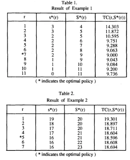
1, we made extensive numerical tests. Among these, we present

two examples below. Usually the processing time for a typical manufacturing system has a very small coefficient of variation: it is almost deterministic. However, if the facility fails during a processing time, then the time to repair the facility could be accounted for in the processing time. In the first example, we consider such a distribution. Thus, in example 1, the processing time is a sum of the actual processing time of an item, plus the repair time of the failure that might occur during the processing of the item. In example 1, we assume that the actual processing time has a constant value, 3. The probability that the machine fails during a processing of an item is 0.05. The repair time to fix the machine follows an exponential distribution with mean 10. The setup time is assumed to have a deterministic value 20. Other parameter values are given as ). = 0.1, K = 500, Ch = 1 and Cb = 10. In example 2, the setup time is assumed to follow an exponential distribution with mean 20 and the processing time is assumed to follow a uniform distribution in the range [8,10]. Other parameter values are given as ). = 0.1, K = 500, Ch = 1 and Cb = 30. Note that example 2, compared to example 1, represents the situation where the utilization of the production facility is very high and backorder cost is high. The results of the policy comparisons for these two test examples are presented in tables 1 and 2. In each table, to show the behavior of the cost functions, the values of 1',8*(1'), S*(r) and TC(r, S*(1')) are given for each value of r. The optimal policy found by the algorithm for example 1 is 1'* = 7 and S* = 9. This policy is a global optimum because S*(1') increases at l'

=

1, while 1'* is 7. The policy,

1'*

=

5 and S* = 21, obtained for example 2 is also a global optimum because the setup time follows an exponential distribution. Although only two distributions for the setup time are demonstrated in the examples, many other distributions can be implemented easily because bj can be expressed in closed form for many distributions of practical interest.

5. Conclusions

We have introduced the (1', S) control policy for production/inventory systems where items are produced on an item by item basis with completed items going directly into in-ventory. The (1', S) policy considered in this paper is a pull type policy which is very useful in situations where the production facility is used for some secondary work during a non-production period. In this study, we assume that processing time to produce an item follows a general distribution and each time production is initiated a random amount of setup time is taken. For this system, under a linear cost structure, we obtained an expression for the expecteCl cost per unit time for given control values and developed an extremely simple, yet efficient search procedure to find the optimal control values. In devising search procedures,

The Optimal (r,S) Policy 157

unimodality property as well as the recursive nature of the cost functions was effectively ex-ploited. Although proofs of optimality were presented only for the system with exponential setup times, a solution guaranteed to be a global optimum can be always obtained with very little additional computation.

Table I. Result of Example 1 r s*(r) S*(r) TC(r,S*(r)) 1 3 4 14.303 2 3 5 11.872 3 2 5 10.595 4 2 6 9.751 5 2 7 9.288 6 2 8 9.063 *7 2 9 9.000 8 1 9 9.043 9 1 10 9.084 10 1 11 9.200 11 0 11 9.736

( *

indicates the optimal policy)

Table 2. Result of Example 2 r s*(r) S*(r) TC(r,S*(r» 1 19 20 19.301 2 18 20 18.897 3 17 20 18.711 4 17 21 18.604 *5 16 21 18.596 6 16 22 18.608 7 16 23 18.694

( *

indicates the optimal policy) Acknowledgment

The author is grateful to the anonymous referees for their helpful and constructive com-ments. This study was partially supported by grants from the Korea Research Foundation in 1991.

Appendix: proof of lemmas 2.1 and 2.3 Lemma 2.1

The term fk,k+l is expressed recursively as U

!k,k+l =fk-l,k - (1 _ p) Cb , for k

S

0,

1 l o o k U 00

fk-l,k

+

--{~fk-l

+ -:\

L

qj(Ch

+

Cb) -

L

qj~fk-j

+

~Cb

L

qj}, k :> 0,

with an initial value

Cb AU(2) _ _

f-l,O == (1 _ p) {2(1 _ p)

+

u}, where p = AU.

Proof

let Ek denote the expected cost incurred during a processing time that is initiated with

k items in inventory. Then fk,k+l is expressed as

(A.1)

00

fk,k+1

=

Ek

+

L

Qjfk+l-j,k+1. j=l

The term Ek in equation (A.1) is obtained by the following equation (The proof can be found in Srinivasan and Lee[9]).

If k ~ 0, (A.2.a) where if k

<

0, (A.2.b) with 1 k

hk+l = ILk

+

;:(1 -

L

qj), with hk = 0 for k ::; 0, j=O

AU(2) Eo = -2-q·

Let us define b.Ek = Ek - Ek-l. Then, from equation (A.1), we obtain (A.3)

00

b.fk = IlEk

+

L

qj(fk+l-j,k+1

+

fk-j,k). j=l

After a little algebra using equation (A.3), b.fk - Ilfk-l is expressed as

00

Ilfk - Ilfk-l = IlEk - /}.Ek-l

+

L

Qj{(fk+l-j,k+1 - fk-j,k) - (fk-j,k - fk-l-j,k-d} j=l

(AA)

00

= IlEk - b.Ek-l

+

L

qj(llfk - Ilfk-j). j=l

Note that the last term in equation (AA) consists of infinite terms. However, b.fk - b.fk-l can be simplified without these infinite terms as described below.

Let Dk denote the time period from the epoch when the inventory level reachesk to the epoch when the inventory level is raised to k

+

1 for the first time. Note that the length of Dk is equivalent to one busy period in an M/C/1 queueing system, hence, from the well known busy period analysis, the expected length of Dk is ft/(l - p) where p = Aft. If we

The Optimal (r,S) Policy 159

compare the inventory level during Dk and the inventory level during Dk+1, the inventory level during Dk has the same stochastic path as the inventory level during Dk+1 if one item of inventory is added to the inventory level during Dk throughout this period. Consequently,

if k

<

0, the inventory level during Dk has only one more shortage than the inventory level

during Dk+1 on the average. Thus, for k

<

0,

(A.5) f:l.fk = h,k+! - fk-l,k = - (1 _ it p) Cb·

If we solve equation (A.4) in terms of

f:l.h

and substitute f:l.fk = - ( it ) Cb for k

<

0, we 1-p

obtain the following recursive equation:

(A.6) 1

k k it

f:l.fk = -{f:l.fk-1

+

f:l.Ek - f:l. E k_1 --

L

qjf:l.fk-j - (1 -

L

qj) ( _ ) Cb},

qo j=l j=l 1 P

where from equation (A.2), (A.7)

1 k-1

f:l.Ek - f:l.Ek-1 = (hk - h k - 1)(Cb --Ch) = ~(1 -

L

qj)(Ch

+

Cb)· j=O

Now, from equation (A.6), the term f:l.fk for k ~ 0, can be computed recursively using the initial value f:l.f -1 = - ( it ) Cb, and hence, f:l.fk for any k can be computed. From this,

1-p h,k+1 is obtained recursively as 1 1 k-1 k fk,k+1 = fk-1,k

+

-{f:l.fk-1

+

~(1 -

L

qj)(Ch

+

Cb) -

L

qjf:l.fk-j qo j=O j=l k it - (1 -

L

qj) ( ) Cb}· j=l 1 - P

The initial value i-1,0 can be obtained directly from the fact that f-1,0 is just the expected total cost incurred during the busy period in an associated M/C/1 queueing system where the unit waiting cost per customer is Cb.

Lemma 2.3

The term

C\

is obtained from

with an initial value,

v

Note that the expected length of period 2 initiated with k items in inventory is - - (refer 1-p to equation (2.14)). We use the same argument as we used in the proof of lemma 2.1. Then by comparing the stochastic path of the inventory level during period 2 initiated with k

inventories with that of the inventory level during period 2 initiated with k - 1 inventories,

-

-

-

v

Ck is expressed as Ck = Ck-l - Cb ( ). I-p Case k

>

0: (A.8) 00 Ck

=

Ck--1 + Tk-1 -

E

bj Tk_l_j j=O k-l 00 = Ck--1

+

Tk-1 -

E

bj Tk-l-j -

E

bj Tk-l-j. j=o j=k

The last term in equation (A.8) consists of infinite terms, which can be handled as follows. Let Tk denote the time period during which the expected cost of Tk is incurred. Then, there is a relationship that the length of Tk is equivalent to one cycle in an associated M / G /1 queueing system. Hence, from the known result of an M / G /1 system, the expected length of Tk is (1 _1 p)>..' Using this fact, we can express Tk for k

<

0 as a function of L l as

follows:

(A.9) Tk

=

T -1 - (k

+

1) (1 _ 1 p )>.. Cb, for k

<

O. Now the infinite terms in equation (A.9) can be expressed as

(A,10)

By sUbstituting (A.IO) into (A.8), we obtain the desired result. The term

Co

which is used as an initial value can be computed in a similar way. From Fubini's theorem, ~o is obtained

>..v(2) it

as -2-Cb' Note also that !k,k+l = !-1,0 - (1

+

k\ _ p Cb, for k

<

O. Using these facts

Co

is expressed as 00

Co

= ~o

+

E

bj!_j,o j=l 00 j-l

-=~o+EbjE{f-l,O+(j-I-k)I:

Cb} j=1 k=O p it 00 j(j - 1) = ~O

+

!-I,O>"V

+

~Cb

E

bj 2 P j=1 >..v(2) p>..v(2)

+

2pv >..2vu(2)

=

- 2 - Cb

+

2(1 _ p) Cb

+

2(1 _ p)2Cb.

o

The Optimal (r,S) Policy 161

References

[1] Buzacott, J.A. and Shanthikumar, J. : Stochastic Models of Manufacturing Systems. Prentice-Hall, New Jersey 1993.

[2] Federgruen, A. and So, K. : Optimality of Threshold Policies in Single Server Queueing Systems with Server Vacations. Adv. Appl. Prob. Vol. 23 (1991), 388-405.

[3] Federgruen, A. and Zheng, Y. S. : Characterization and Efficient Computation of Op-timal Policies for General Inventory Systems Endogenously Supplied by a Single Server Production Facility. Technical Report, Graduate School of Business, Columbia Univer-sity, USA 1991.

[4] Gavish, B. and Graves, S. C. : A One Product Production/Inventory Problem Under Continuous Review Policy. Opns. Res. Vol. 28 (1980), 1228-1236.

[5] Gavish, B. and Graves, S. C. : Production/Inventory Systems with a Stochastic Pro-duction Rate under a Continuous Review Policy. Camp. & Opns. Res. Vol. 8 (1981), 169-183.

[6] Heyman, D. P. : Optimal Operating Policies for M/C/l Queueing Systems. Opns. Res. Vol. 16(1968), 362-382.

[7] Ross, S. M. : Applied Probability Models with Optimization Applications. Holden-Day, Sanfrancisco 1970.

[8] Scarf, H. : The Optimality of (s, S) Policies in the Dynamic Inventory Problem, in K. Arrow, S. Karlin and P. Suppes (Eds.), Mathematical Methods in the Social Sciences. Stanford University, Stanford 1960.

[9] Srinivasan, M.M. and Lee, H.S. : Random Review Production/Inventory Systems with Compound Poisson Demands and Arbitrary Processing Times. Management Science Vol. 37(1991), 813-833.

[10] Tijms, H.C. : An Algorithm for Denumerable State Semi-Markov Decision Problems with Application to Controlled Production and Queueing Systems, in Recent Developments in Markov Decision Theory, ed. R. Hartley et al. Academic Press, New York 1980. [11] Veinott, A. : On the Optimality of (s, S) Inventory Policies: New Condition and a Proof.

J. SIAM Appl. Math. Vol. 14(1966), 1067-1083. Hyo-Seong Lee

Department of Industrial Engineering Kyung Hee University

Kiheung, Yongin-goon, Kyunggi-do 449-900, Korea