AN INTEGER RESOURCE ALLOCATION PROBLEM WITH COST CONSTRAINT

Journal of the Operations Research Society of Japan

Vol. 41, No. 3, September 1998

AN INTEGER RESOURCE ALLOCATION PROBLEM WITH COST CONSTRAINT

Ryusuke Hohzaki Koji Iida

National Defense Academy

(Received August 1, 1997; Final April 20, 1998)

Abstract This paper investigates a non-linear integer programming problem with an exponential objective function and cost constraints, which is a general model and could be applied t o the assignment problem or the search problem. As a representative example, we consider a following problem of assigning m types of missiles to n targets. The value of target i is V, and the single shot kill probability (SSKP) of a j-type missile to target i is ,Bij = 1 - exp(-a^) where aij

2

0. Denoting the number of j-type missiles assigned to target i by n ~ , the expected destroyed value is given by _{V, {l - exp(-} a y n i j ) } . If a unit price of j-type missile is c, and the total cost of missiles is limited by C, we have cost constraints

G

cj _{n'j 5 C .}

To this problem which is NP-hard, we propose two methods, the dynamic programming method and the branch and bound method. An approximate algorithm and an estimation of the upper bound of the objective function are incorporated in the branch and bound method. Each of these methods has its characteristic merits for the computational time. We clarify their characteristics through the sensitivity analysis by some examples in this paper.

1. Introduction

This paper investigates a non-linear integer progra,mrning problem with an exponential objective function a,nd cost constraints, which is frequently encountered in a variety of a,pplica<tion areas, and proposes new methods for solving the problem. For example, we consider a following problem of a,ssigning m types of missiles to n targets. The value of ta,rget i is

K

a,nd the single shot kill probability (SSKP) of a j-type missile to target i is

fii, = 1 - exp(-a,,) where a,,

2

0. Denoting the number of j-type missile assigned to

target i by nrij, the expected destroyed value is given by

K

{l

- exp(-

G

~ ' t j n ~ j ) . If

I

a unit price of j-type missile is

c,

a,nd the tota,l cost of missiles is limited by

C ,

we ave exist c~nstra~ints

^Fl

c,

^,'L,

n,,

5

C. R,.H.

Nickel et a.1. [5] incorporated a. similarr model in his uniformly ajssignment model with multi-types of missiles arnd multi targets. Since they dealt with their constraints as the condition not on cost but on the numbers of missiles, their optimiza/tion problem was slightly different from our problem and ~ornpara~tively easily solved.

We can find a similar model in the search problems. A searcher wants to rna,ximize the proba,bility of detecting a stationary target which hides himself in one of n cells. The location of the target is not known with a certa,inty and the prior pr~ba~bility of the target's existing in cell i is e~tima~ted by pi. The searcher is given T search time points, t = 1 , 2 , - -

,

T , when he can look into whichever cell as ma,ny times as he likes. At time point t, he can detect the target wit>h proba,bility

pit

(= 1 - e ~ p ( - - a ~ ) ) by looking into cell i if the target

is there. On the other ha,nd, a look into a cell costs et at time t and the total cost is limited by C. When the searcher ha,s the strategy of looking into cell i n2 times at time

t ,

Integer Resource Allocation Problem 4 71

the detection probability and the cost constraint are given as

G

pi {l - exp(- @an^)}

and

^El

Q nit

<:

C,

respectively.

A

problem of distributing discrete search resources

was studied by J.B. Kadane[6]. He proposed a little different model where the searcher took

only a look into a cell at every time and the look cost varied depending on the number of past looks, and the detection probability was to be maximized. His problem is different from our problem and it is able to be reduced to the problem of optimizing the number of looks at one time point and to the knapsack problem in consequence.

The above two models, the missile assignment problem and the search problem have the

same objective function and the same constraints on variables.

A

purpose of this paper is

not to solve the real-life missile assignment problem or the practical search problem but to propose some new methods of giving an exact solution to this type of problem with an exponential objective function and cost constraints, which has not been studied clearly so far.

Our problem stated above becomes the knapsack problem in the case of n = 1. It

reminds us tha,t our ~roblem is NP-hard. In this paper, the dynamic programming method

and the branch and bound method are proposed to solve our problem. In the next section, we formulate our problem as an integer programming problem. Two exact methods, the dynamic programming method and the branch and bound method are discussed in Sections

3 and 4, respectively. In Section 5, a numerical exa,mple is examined to investigate the alternative strategy about which of special use missiles or general-purpose missiles should be adopted. Other numerical examples are used to estimate the performance of two methods concerning with the computational time.

2.

Formulation of Problem

Here, noting that the same model is possible to some problems in other fields as stated in the introduction, we take a, missile assignment model as one of representative examples and

formulaic it as an integer programming problem.

(1) A defender has n targets with their values

{K

>

0

,

à = l ,

- -

,

n}.

(2) An attacker has m types of missiles and a j-type missile has the capability of SSKP

0

<

By <

1 to target z.

(3) A unit cost of j-type missile is c,

> 0 and the total cost of the attacker is limited by

C

>

0.

(4) The attacker wants to find an optimal assignment of his missiles of maximizing the

expected destroyed value of targets .

For convenience, we replace

/3a

with 1 - exp(-aij) where a y

;>

0. Denoting the number

of j-type missiles assigned to target z by variable nq, we obtain the kill probability of

target z, 1 - (l -

,Bi,)""

= 1 - exp(- a y n u ) and the total cost,

G,

c, nij.

Therefore, our problem is formulated as the following integer programming problem (PO).

Z ^

is a set of non-negative integers.

n ( m 1

+

4 72 R. Hohzaki & K. Iida

suffix. One of the earlier studies about the assignment problems of missiles is Manne's[4] where the objective function has one suffix and the total number of missiles is restricted. Another one is Lemus7s[3]. He studied the objective function given by Eq.(l) with the constraint upon the number of missiles and proposed an approximate algorithm. Nickel[5] extended it and analyzed the effective use of the general-purpose weapon. Concerning with

multiple resource allocation problems with the objective function of Eq.(l), some studies

have been published so far but constraints are given only upon the number of resources[?].

As you c m imagine, cost coefficients {c,} make this problem

(PO)

difficult to solve.

In the case of n = 1, the problem

(PO)

becomes a knapsack problem of maximizing

Gl

alinl,. It proves that our problem is NP-hard. Assuming that parameters {ci, j =

1,

.

,

m}

are rational numbers, we multiply both sides of inequality (2) by the least common

multiple of their denomina,tors and then make coefficients {c,} be integers. Hereafter we

treat {c,} as positive integers.

3. Solution

by

Dynamic Programming Method

We define a subproblem of

(PO)

with the number of targets k

<:

n and cost limit

D

as

follows.

k m

E E

cjnifi

D,

n~ 6

Z+

. ( 4 )

1x1 j=1

We define the optimal value of a kna,psack problem by

l

+

Fk-l(D -

Qk)]

Many studies about the integer knapsack problem have been cumulated so far. Gilmore[l] proposed the dynamic programming algorithm by using the periodicity of the knapsack

function. By his study, vk (Q), Q = 0,1,

- -

,

C

are given as by-products in the process of

computing vk

(C)

[2]. We use recursively Eq. (6) varying k ==Â¥ 1,

- - ,

n,

D

= l,

- - -

,

C

to

obtain

K(C)

in consequence. Denoting the complexity of computing vk(C) by knap(C),

the computation of

&(C)

takes the complexity of order 0 ( n

-

(knap(C)

+

C2)). We call the

dynamic programming method the DP method for short.

4. Solution by Branch and Bound Method

As known from recursion (6), cost Qn permitted to missiles which are designated to target n ought to be determined at the first step for evalua,ting &(C). If Qn is determined,

then the decision making of Qn-1 within residual cost

C

- Qn is the second step. These

decision making points look like nodes on an enumeration tree used in the branch and bound method. We propose the branch and bound method by this idea. I t is essential to

find an effective bound estimakion and an appro~ima~te solution as exactly as possible for

the efficient execution of this method. The a,pproximate algorithm is discussed afterward.

Our branch and bound method proceeds as follows. A root node branches to

C+

1 nodes,

I(1) = {O, 1,

- -

,

C},

each of which indicates the cost constraint Ql to be designated to target

Integer Resource Allocation Problem 4 73

cost constraint Q2 for target 2. In the result, a n-ply layered tree is generated as an

enumeration tree. On the sth layer, Ql, Q2,

- -

,

Q, are already given but Q,+l,.

,

Qn

are not determined yet. By given Ql, Q2,

-

,

Q,, the maximum of the expected destroyed

value of targets 1, 2,

- - -

,

S is calculated, which is saved in ~ ( s ) in the algorithm. In Q(s),

Qi is saved. Because the distribution of the residual cost

C

- Q(s) to targets S

+

1,

- - ,

n

is not determined yet, the problem of giving the maximum of the expected destroyed valhe of targets S

+

1,

- - -

,

n,

By an approximate algorithm, find a tentative value of the objective function

and store it in f c . Set Q(0) = 0, ~ ( 0 ) = 0, s = 1 and

I

(l) = {O, 1,

- ,

C}

and

go to (Step2).

Select a value from I ( s ) , store it in Q, and set Q(s) = Q{s - 1)

+

Q,. Solve the

following knapsack problem

Gs(C - Q(s)) := max

Vicf

y > k j n y

{£

(Ll

)

and calculate v(s) by i;(s - 1)

+

V.

-

f (vS(Qs)).

If s equals to n , go to (Step7).

Solve a relaxed problem of G,

(C

- Q(s)) to find

G,

(C

- Q(s)) and estimate an

upper bound by setting

G

= ~ ( s )

+

GS(c

- Q(s)).

If

G

S

f c , go to (Step4).

If

G

>

f c and the relaxation problem has an integer optimal solution, set f c =

G

and go to (Step4). In the case of

G

>

f c and non-integer solution, go to (Step6).

Set I ( s ) = I(s) - {Q,}.

If /(S) becomes an empty set, set S = S - 1 and go to (Step5). Otherwise, go to

(Step2).

If S equals 0, terminate. Current f c gives the optimal value.

Otherwise, go to (Step4).

n m

E

x ~ j n t j S C - Q ( ~ ) ~ n k j ~ z "

k=s+l j=1

,

Increase S by one or set S = S

+

1.

If s equals n, set

I

(S) =

{C

- Q(s - l)}. Otherwise, set

I

(S) = {0, 1,

- -

,

C

-

Q(s - l)}. Go to (Step2).

If f c

<

v{n), set f c = ~ ( n ) . Go to (Step4).

is difficult to be solved, where we use notation f (X) := 1 - exp(-X) for convenience. Instead

of rigidly solving the problem, we can estimate an upper bound & ( C - ~ ( s ) ) of G,(CÑQ(s) by solving a problem of relaxing integer variables {nkj} to real numbers and furthermore

estimate an upper bound of the optimal value of the original problem _-

(PO)

by

G

= B(S)

+

G,(c

- Q(s)) .

_{( 7 )}

Now we discuss the approximate algorithm and the estimation of an upper bound of the objective function. Hereafter the branch and bound method is occasionally called the BAB method for short.

4.1 Approximate algorithm

For emphasizing the missile assignment {ran, z = 1,

- - - ,

n, j = 1,

-

.

,

m}, we provide another

4 74 R. Hohzaki & K. Iida

Consider another assignment { n g . Only the specific va,ria,ble n h is different from nkz, that is % l + l , and all other elements are the same afs {nn}. Then the ratio of the value increment

of the objective function to cost increment is given by the following eq~a~tion.

Hn({n'.,})

- &({ÈG} & ( l - exp(-akl)) m

Ykl

-

- - _{- exp}

Ci Cl J=l

This ratio gives us a measure of efficiency about the increment of the number of missiles. Now we propose an approximake algorithm, say a greedy algorithm, as follows. Starting from

{ n i ~ } =- {O}, TIJU which sahisfies ~onstra~int (2) and maximizes ym is increased by one. This

process is repeated until constraint (2) is violated. As known from Eq.(9), the increment

of

m

makes each of ratios {ykj, J = 1,

.

-

-

,

m} multiplied by exp(-W). Furthermore, the

ordering among ykj is never changed for j = 1,

.,

m. n this process, if the increment of

nkl is not permitted by cost constraint, which means more cl is beyond the cost permission,

{U

i =

l,

- -

-

,

n,}

are no longer candidates for being increased. We itemize our greedy

algorit hm as follows.

For i=l,

-

-

,

n , j = l,

-

,

m, calculate the measure of efficiency by

Initialize parameters as follows.

in,,} = {O}

,

B

=C,

F=

{ 1 9 2 , - - - , m } .

Set

F = F - { j e F l

B - c j < 0 } .

If

F is

0,

then terminate. Current {nij} gives an approximate solution

Select (k, 1) by

yki = max

jâ F,z

and revise parameters as follows.

4.2 Upper bound estimation

Here we solve the relaxation of Gs(C - Q ( s ) ) in (Step3) of the

BAB

procedure. To avoid

the complicated present ation, we discuss the relaxat ion of (4), which is essentially the same

problem as Gs

(C

- Q ( s ) ) .

m

l - exp(- aijnij)

<

D,

ni,

>

I)] . (10)

j=l

An optimal solution is given by the following theorem.

aij* (i) Q i j

Theorem 1. For i = l, -

- -

,

k, set oi = = max - . Then an optima,l solution

cj* ( i ) 3 C j

{nij, Z = 1,

-

-

,

k, j = 1, - -

,

m} of the relaxa,tion (10) is presented b y the following formulae.

nq = 0, ]^

m)

.

A is a Lagrangean multiplier uniquely determined b y the next equation.

[x}+

denotes max{0, X}.

Integer Resource Allocation Problem

It is easy to solve this maximization by using the Kuhn-Tucker condition.

A

Lagrangean

function L({^}) is defined by the following.

k / k \ k

The following conditions are necessary and sufficient for an optimal solution.

9L

- = ViOie-<T^qi -

A

+

ui = 0, i= l , . . . , k

,

9Qi

(16) viqi = O , Ã ˆ l , . . . , k

,

k (18)

- y q 2 = D .

2=1 (19)

Using these conditions, qi

>

0 results in vi = 0 and b e u i q i = A. The case, of qi = 0 results

in v 2 _

>

0 and Voie-^ =

A

- vi

5

A. Therefore, an optimal solution of {qi} is present,ed

by the following equation.

1

+

q2 -

log?]

0-2 (20)

In the result, an optimal solution of

{n^}

is given by Eqs. (l l) and (12). Multiplier A is

determined uniquely by Eq.(19) or

Q.E.D.

We explain about a concrete procedure of computing inij} and F k ( ~ ) . Without loss of

generality, assume that

vial

>

>

-

>

K0-k. After finding

1

=

Via\

= maxi

VG,

A

=

mmi e-ciD

z 2

,

Eq. (21) holds for a finite

A

satisfying

A

>

A

>

A

because

g(A)

= 0, g(A)

2

D

and g(A) is non-increasing for variable A. Therefore, we can determine

I*

uniquely,

I*

satisfying g(&*m*)

<

D

g(l$*+lal*+l) or I* = k satisfying g(K0-k}

< D. Then Eq.(21)

becomes the following.

R. Hohzaki & K. Iida

5. Numerical Examples

Here, we investigate the characteris tics of optimal solutions and the computational efficiency of the proposed met hods. We take missile assignment problems as comprehensive examples. By the first example, we investigate the alternative strategy among missiles for special use and for general purpose. By the second a,nd the third examples, the sensitivity of the

proposed two methods are analyzed for the change of the cost limit

C

and the number of

targets or missiles in terms of computat ional time.

5.1 _{Alternative strategy among some types of missiles}

Here we examine some characteristics of optimal solutions. Generally speaking, if the con- straints of the integer problem are loose, optimal integral solutions become little different from optimal continuous solutions of the problem relaxed by changing integral variables to continuous ones. Then, in some examples, we impose tight constraints on available total cost

so that small

C

is set comparing with the unit cost

c,

and elucidate interesting properties

of optimal integral solutions.

Consider 4 targets with their values

V\

<:

<:

V3

<:

V4

and 5 types of missiles, that

is, n = 4 and m = 5. The fifth type of missiles is manufactured for general purpose. It

is comparatively effective to each of 4 targets a,nd cheap. Each of other types of missiles is most effective to a specific target and a little expensive. The 2-type missile for special

purpose has the highest SSKP to target 2 but lower SSKP to other targets. We analyze the

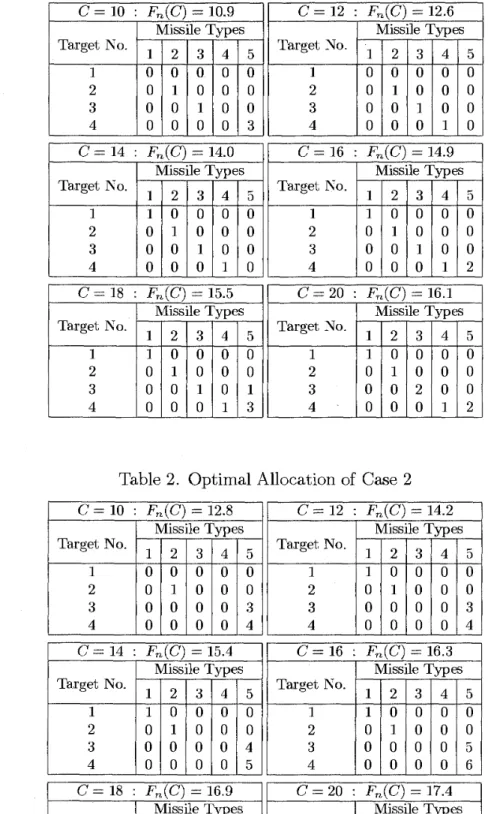
optimal assignment of missiles by va,rying parameters. (Casel) This is a basic case.

0 Target value:

Vi

= 2,

V2

= 4,

V3

= 6,

V4

= 8

0 Unit prices:

cl

= 2,

c2

= 3,

c3

= 4,

c4

= 5,

c5

= 1

o SSKPs: f t i = 0 . 7 , f t , = 0 . 1 ( G j ) , i , j = 1 , - - - , 4 ,

ft5

=0.2, i = 1 , - - . , 4

Changing the total cost limit to

C

= 10,12,14,16,18,20, optimal assignments

{riij}

are presented by Table 1. As seen from this table, the optimal solution consists of assigning special-purpose missiles at first and then covering residual cost permission by cheap missile for general purpose.

(Case2) In this case, only SSKPs of general-purpose missile of Case 1 increase a little and other parameters are the same as Case 1. An optimal solution is given in

Table 2.

0 SSKPS: ,&j = 0.3, i = 1, - -

-

, 4

The optimal assignment changes as follows. The assignment of the 1st and 2nd

types of missiles is preferable, which is the same as Case 1, but the adoption of

more expensive 3rd a,nd 4th types of missiles is likely to be restrained. Instead of the 3rd a,nd 4th types of missiles, many general-purpose missiles are concentri- cally assigned to targets 3 and 4 in order to assure the high expected destroyed value.

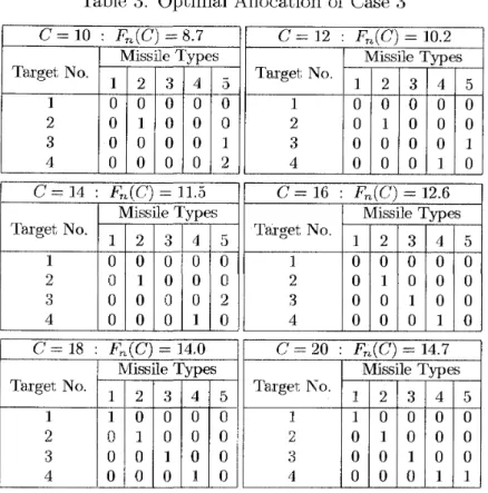
(Case3) This is the case in which unit prices of missiles of Case 2 increase by one and other parameters are the same as Case 2. Optimal solutions are shown in Table

3.

Unit prices:

cl

= 3, c2 = 4,

c3

= 5, c4 = 6, CQ = 2

In this example, the general-purpose missile plays both of a complementary and

Integer Resource Allocation Problem

Table 1. Optimal Allocation of Case 1

Table 2. Optimal Allocation of Case 2 r C= 10 : Fn(C) = 10.9 C = 12 : Fn(C) = 12.6 Target No. 1 2 3 4 C = 14 : FJC) = 14.0 Target No. 1 2 3 4 Missile Types 1 2 3 4 5 0 0 0 0 0 0 1 0 0 0 0 0 1 0 0 0 0 0 0 3 Target No. 1 2 3 4 C = 16 : Fm(C) = 14.9 Missile Types 1 2 3 4 5 0 0 0 0 0 0 1 0 0 0 0 0 1 0 0 0 0 0 1 0 Missile Types 1 2 3 4 5 1 0 0 0 0 0 1 0 0 0 0 0 1 0 0 0 0 0 1 0 Target No. 1 2 3 4 C = 14 : FJC) = 15.4 C= 18 : Fn(C) = 16.9 Missile Types 1 2 3 4 5 1 0 0 0 0 0 1 0 0 0 0 0 1 0 0 0 0 0 1 2 Target No. 1 2 3 4 C= 16 : Fn(C) = 16.3 Target No. 1 2 3 4 C = 2 0 : Fn(C) = 17.4 C= 18 : Fn(C) = 15.5 Missile Types 1 2 3 4 5 1 0 0 0 0 0 1 0 0 0 0 0 0 0 4 0 0 0 0 5 Target No. 1 2 3 4 Missile Types 1 2 3 4 5 1 0 0 0 0 0 1 0 0 1 0 0 0 0 6 0 0 0 0 6 Target No. 1 2 3 4 Target No. 1 2 3 4 C = 20 : Fn(C) = 16.1 Missile Types 1 2 3 4 5 1 0 0 0 0 0 1 0 0 0 0 0 0 0 5 0 0 0 0 6 Missile Types 1 2 3 4 5 1 0 0 0 0 0 1 0 0 2 0 0 0 0 6 0 0 0 0 7 Missile Types 1 2 3 4 5 1 0 0 0 0 0 1 0 0 0 0 0 1 0 1 0 0 0 1 3 Target No. 1 2 3 4 Missile Types 1 2 3 4 5 1 0 0 0 0 0 1 0 0 0 0 0 2 0 0 0 0 0 1 2

R. Hohzaki & K. Iida

Table 3. 0ptima)l Alloca,tion of Case 3

C = 20 : Fn(C) = 14.7

1

Missile Types T a , r g i No.

ml

1 2 3 4 5 1 0 0 0 0 0 1 0 0 0 0 0 1 0 0 4 0 0 0 1 1

more 4th type of missile or two more 1st type of missiles instea,d of 3 general- purpose missiles. In this case, the genera,l-purpose missile is of main use. I11 cases of other cost limits, it is of complementary use. The usage of the general- purpose weapon depends not only on its cost-performance but also on other missiles' cost-performance. In addition, the solution is perturbed a little by the attribute of its being integer.

5.2 Computational analysis for two methods

Two methods, the DP method a,nd the BAB method, are proposed in the previous sec-

tion. Here, we are interested in comparison between the computational time of them.

A

mainframe computer HITACHI S3600/120A and FORTRAN

77

a,re used as the computer

ha,rdwa,re arnd language.

(1) Change of cost permission

With varying the cost limit

C

from 40 to 200 in Case 1, CPU-time(seconds) for both

methods are measured and presented by Table 4. In data for the BAB method, CPU- time of using the Greedy algorithm and solving the relaxed problems are all included. For the sake of comparison, the result by the total enumeration method (TE method) on the enumerakion tree and the result by the greedy algorithm are written ako. Not only CPU-time but also the relaiive error of the value of the greedy solution to an optimal one a,nd the number of bra,nches on the enumera,tion tree are both obtained

for the BAB method. From the discussion of Section 3, it is comprehensible that

computational time increases as

C

increases for the DP method. However, for the

bra,nch and bound method, it depends 011 the precision of the greedy solution a,nd the

efficiency of the bounding process and so it varies case by case. From this example,

the increa,se of CPU-time appea,rs in the case of

C

= 40 120. On the contrary,

Integer Resource Allocation Problem

Table 4. CPU-Time(sec.) of Case 1 with varying

C

Method DP

BAB

Greedy

tha,t the relative error of the greedy solution becomes extremely small, which makes the bounding process more efficient a,nd the number of branches more less. I11 Table

4,

Fn(C)

in the case of

C

>

100 is nearly equal to the optimal value without cost

constra,int, which is Vl

+ +

V3

+

V4 = 20. Therefore, the optimal condition in the

case of large

C

is not so tight that there are ma,ny good solutions around the optimal

one a,nd perhaps the greedy solution is one of them. This computational characteristic

afbout the

BAB

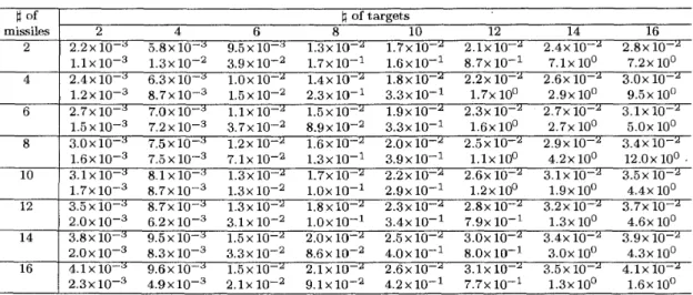
method generally appears in other cases.

Change of the number of targets or the number of missile types

Here, we analyze the sensitivity of n and m to the computa,tional time for two methods.

We vary n from 2 through 16, m from 2 through 16 with fixing

C

= 50. Other

parameters are determined as follows. For a combina,tion of n and m, we randomly

select the unit prices of ea,ch type of missile values of targets Ks afnd SSKPs /^,S,

during [l, 101, [l, 101 a,nd [0.0 1,0. 91, respectively. By this way, we make 10 problems

and measure CPU-times for solving these problems by each of two methods. CPU-

times in Table 5 are presented by the mean value. The upper figures are data for the

Items CPU-Time

CPU-Time

T E

Table 5. CPU-Time(sec.) with varying n and m

Cost permission : C 40 60 80 100 120 140 160 180 200 5 . 0 ~ 1 . 0 ~ 1 . 7 ~ 2 . 5 ~ 3 . 6 ~ 4 . 8 ~ 6 . 1 ~ 7 . 6 ~ 9 . 2 ~ 1 0 - ~ 10-2 I O - ~ 1oà 1 0 - ~ l o à 10-2 10-2 I O - ~ 1 . 5 ~ 2 . 2 ~ 4 . 6 ~ 6 . 1 ~ 9 . 3 ~ 7 . 9 ~ 2 . 7 ~ 7 . 5 ~ 8 . 3 ~ I O - ~ 10-a 1 0 - ~ 1 0 - ~ 1 0 - ~ 10-' 1 0 - ~ l"-' # of branches CPU-Time Relativeerrors tt of 1 of targets 851 1183 2661 3497 5386 4167 983 101 101 3 . 8 ~ 5 . 1 ~ 6 . 8 ~ 8 . 2 ~ 9 . 7 ~ 1 . 1 ~ 1 . 3 ~ 1 . 4 ~ 1 . 6 ~

l o p

lop4 I O - ~ 10-< 1 0 - ~ lop3

lom3

1 . 5 ~ 4 . 4 ~ 1 . 1 ~ 3 . 1 ~ 7 . 2 ~ 1 . 7 ~ 3 . 1 ~ 9 . 4 ~ 2 . 9 ~

1oy2 10-3 10-a I O - ~ 10-Â 10-Â I O - ~

io-Â

low8

CPU-Time

o f b r a n c h e s

4 . 5 ~ 1 . 4 ~ 3 . 2 ~ 6 . 1 ~ 1 . 0 ~ 1 . 6 ~ 2 . 4 ~ 3 . 5 ~ 4 . 7 ~ 1 0 - ~ 10-I 10-I 10-l loo 10 10 10 10 2 . 6 ~ 8 . 1 ~ 1 . 9 ~ 3 . 6 ~ 6 . 1 ~ 9 . 6 ~ 1 . 4 ~ 2 . 0 ~ 2 . 8 ~ 104 104 105 105 105 105 106 106 106 missiles 2 4 2 4 6 8 10 12 14 16 2 . 2 ~ 1 0 - ' 5 . 8 ~ 1 0 - ~ 9 . 5 ~ 1 0 - ^ 1 . 3 ~ 1 0 - ^ 1 . 7 ~ 1 0 ~ ' 2 . 1 ~ 10-^ 2 . 4 ~ 10-^ 2 . 8 ~ 10-^ 1 . 1 x 1 0 3 1 . 3 ~ 1 0 - ^ 3 . 9 ~ loÑ 1 . 7 ~ 10-l 1 . 6 ~ 1 0 - I 8 . 7 ~ 10-I 7 . 1 ~ 10" 7 . 2 ~ 10" 2 . 4 ~ 1 0 - ^ 6 . 3 x l 0 - ~ 1 . 0 ~ 10-^ l . 4 x l 0 - ^ 1 . 8 ~ 1 0 - X 2 . 2 ~ 10-^ 2 . 6 ~ 10-^ 3 . 0 ~ 10-'¥^

DP method and the lower figures for the

BAB

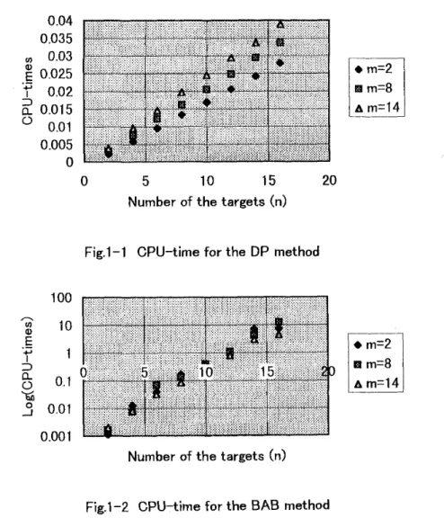
method. Darts for the T E method are omitted since it is clearly inferior to other two methods in atny case.

Figure 1-1 shows how the number of the targets changes the CPU-time by the DP

method in the cases of the number of missile types m = 2, 8 and 14. As you see,

the CPU-time for the DP method shows a linear increase for t,he number of taxgets

n,

which can be estimated from the discussion about the computationa,l complexity in

ection 3. Figure 1-2 shows the cha,nge for the BAB method but it uses the logarithm

as a unit of the axis of ordinate. Thart is, the change of CPU-times is very steep afs

the number of the targets increases. This is by the reason that the enumeration tree

AB

method has the depth of n and the number of the branching or its leaves

is enlarged by the n-th power. However, only concerning with the greedy solution, its

relative error is less than 2.0 x 1 0 2 over the whole cases and the greedy solution can

be obtained easily. In the case of n = 10 and m = 10, the greedy algorithm requires

1.4 X 1 0 3 seconds of CPU-time and yields only 3.4 x 1 0 3 of t'he relative error on the

average.

0 5 10 15 20

Number of the targets (n)

Fig.1-1 CPU-time for the DP method

Number of the targets (n)

Fig.l-2 CPU-time for the BAB method

The number of items in a knapsack problem to be solved on the way is nothing but

Integer Resource Allocation Problem 481

most as much as the number of targets for each method. Therefore the increase of the CPU-time by the increase of m is mainly caused by the fact that the size of the knapsack problem becomes larger. The CPU-time increases as m is larger but its rate

is a little. This is the fact for the DP method, which is seen in Table 5 . For the BAB

method, this is true for small n but not true for large n. In the case of large n, the

change of system parameters m, n,

C,

C % , ay produces much effects on the number

of searched nodes on its large enumeration tree. By this reason, the CPU-time does

not necessarily increase by

m,

remaining its increasing or decreasing rates small. In

fact, the variance of CPU-times becomes larger as n increases, which means that the

CPU-time varies irregularly for each problem. For example, the va,riances for the DP

and the BAB methods are 1.0 X 1 0 " ~ and 0.8 X loV7, respectively, for m = 10, n --= 2

and it becomes 2.0 X 1 0 7 and 8.1 X 1 0 2 respectively, for m = 10, n = 10

In the previous two examples concerning with the computational analysis, it seems that we take comparatively small size of problems. However, as the practical missile assignment problem or the practical search problem, they have enough large size. And it is thought that results obtained by the previous examples give a guideline for applying the proposed methods to other unknown size of problems. Now, we are on the position to itemize the characteristics of the methods.

(1) For the dynamic programming method,

(ii) (iii) (2) For t

(9

(ii) (iii)

Cost constraint

C

indicates a capacity of the knapsack problem as a subprob-

lem. The computational time increases linearly or a little more strongly by the

increase of

C.

The number of the types of missiles indicates the number of items included in

the knapsack problem. The increasing ra,te of the computational time by m is

small.

The number of the targets indicates the number of repeaks in the recursive

equation (6). The increasing rake of the computational time by n is a little more

than linear.

In the middle- and large-size problems for m and n, the DP method is superior

to the BAB method if the exact solutions are required. ie branch and bound method,

The increa,sing rate of the computational time by C is as small ass the DP method.

The effect of m 011 the computational time is small comparing with other sys tem

parameters' effects.

In many cases, the number of targets has the effect of the exponential increase on the computational time because it determines the depth of the enumeration tree.

(iv) In the following case, the bounding procedure of the BAB method has a good ef- fect on the computational time beca,use the relative errors of the greedy solutions to the exact solutions are small.

In the case that the cost constraint

C

is large comparing with the unit

costs {ci} and the number of the missiles can be regarded as real values.

In the case tha,t the SSKPs or { a i j } are large and the small difference of

n i j } has not so laxge effect on the values of the objective function.

482 _{R. Hohzaki} & K. Iida

method and the branch and bound method, to exactly solve the problem. The proposed dynamic programming method is availa,ble to the general objective function that has the

form of

fi

(E>

i o n y ) . For the bra,nch and bound method, if the function fi(-) is

concave and non-decreasing, the relaxed solution might be derived easily as it is done in

Theorem 1.

Our problem is NP-hard, which has been proved, and to shorten its computational time is one of the interesting points. By numerical examples, we can say the followings concerning with the computational time. The dynamic programming method has the linear increasing

feature for the number of targets

n

and the number of types of missiles m, and the squared

increasing feature of the cost permission

C.

For the branch and bound method, there is some

possibility that the computational time decreases in spite of the increasing cost permission.

However it has the steep increasing feature for n , which ought to be improved further. I11

result, the dynamic programming method is superior to the branch and bound method in many cases. However, the greedy algorithm used in the branch and bound method gives

good approximate solutions with small CPU- times, especially in large-size problems.

References

[l] P.C. Gilmore and R.E. Gomory: The theory and computation of Knapsack function.

es., 14 (1966) 1045-1074.

21 R.S. Ga,rfinkel and G.L. Nemhauser: Integer programming (John Wiley & Sons, 1972).

[3] F. Lemus and K.H. David:

A11

optimal all~ca~tion of different weapons to a target

complex. Opns. Res., 11 (1963) 787-794.

Manne:

A

target-assignment problem. Opns. Res., 7 (1959) 258-260.

. Nickel and M. Mangel: Weapon acquisition wit h target uncertainty. Naval Re-

search Logistics, 32 (1985) 567-588.

[6] J.

B.

Kadane: Discrete search and the Neyman- Pearson lemma. J. of Mathematical

Analysis and Applications^ 22 (1968) 156-171.

7 T. Iba,raki and N. Katoh: Resource allocation problem (The MIT Press, London, 1988).

Ryusuke Hohzaki

Department of Applied Physics National Defense Academy 1- 10-20 Hashirimizu, Yokosuka, 239-8686, Japan