PAPER
Hardware-Aware Sum-Product Decoding in the Decision Domain
Mizuki YAMADA†∗,Nonmember, Keigo TAKEUCHI†a),andKiyoyuki KOIKE††,Members
SUMMARY We propose hardware-aware sum-product (SP) decoding for low-density parity-check codes. To simplify an implementation using a fixed-point number representation, we transform SP decoding in the loga- rithm domain to that in the decision domain. A polynomial approximation is proposed to implement an update rule of the proposed SP decoding ef- ficiently. Numerical simulations show that the approximate SP decoding achieves almost the same performance as the exact SP decoding when an appropriate degree in the polynomial approximation is used, that it improves the convergence properties of SP and normalized min-sum decoding in the high signal-to-noise ratio regime, and that it is robust against quantization errors.
key words: low-density parity-check (LDPC) codes, sum-product (SP) decoding, hardware implementation, decision domain, polynomial approx- imation
1. Introduction
Sum-product (SP) decoding[1]is a powerful decoding algo- rithm for binary low-density parity-check (LDPC) codes[2].
In spite of its low complexity, SP decoding can achieve per- formance very close to the channel capacity when an opti- mized irregular LDPC code[3] is used. Furthermore, the channel capacity is universally achievable under SP decod- ing for transmission over general binary-input memoryless symmetric-output channels if spatial coupling[4]is applied to regular LDPC codes. Thus, SP decoding plays a central role in modern coding theory.
In practical communication systems, SP decoding needs to be implemented in hardware devices such as application- specific integrated circuits (ASICs) or field-programmable gate arrays (FPGAs)[5]. In implementing the SP decoding in the logarithm (L) domain, we face two difficult issues[6]–
[8]: (i) how to implement the tanh and tanh−1functions and (ii) how to quantize messages in the L-domain.
To circumvent the former issue (i), decoders based on min-sum (MS) algorithms[9]–[15]have been used instead.
MS-based decoding requires no computations of special functions. Nonetheless, normalized min-sum (NMS) de- coding[16]can achieve almost the same performance as SP
Manuscript received March 26, 2019.
Manuscript revised August 8, 2019.
†The authors are with the Department of Electrical and Elec- tronic Information Engineering, Toyohashi University of Technol- ogy, Toyohashi-shi, 441-8580 Japan.
††The author is with the Department of Electronic Engineering, National Institute of Technology, Tokyo College, Tokyo, 193-0097 Japan.
∗Presently, with Sharp Corporation.
a) E-mail: [email protected] DOI: 10.1587/transfun.E102.A.1980
decoding for short LDPC codes. However, NMS decoding has two disadvantages: worse decoding performance for long codes and worse convergence property in the high signal-to- noise ratio (SNR) regime especially for short codes.
For the latter issue (ii), uniform quantization enables simple implementations based on fixed-point number rep- resentations. However, it is a challenging issue to design the dynamic range of messages in the L-domain. In many cases, the dynamic range is optimized in a heuristic manner based on numerical simulations. In some cases, the details of quantization are not disclosed. A more sophisticated ap- proach is based on density evolution (DE) [17],[18]. For a given number of quantization bits, Chen et al. [16]used DE to optimize the quantization step or equivalently the dy- namic range, as well as a normalization coefficient in NMS decoding. However, the optimization results depend heavily on the ensemble of LDPC codes, channel statistics, and the number of quantization bits. As a result, optimized NMS decoding is not flexible.
In this paper, we propose SP decoding in the decision (D) domain instead of the L-domain. The D-domain is defined as the image of the tanh function, i.e. the interval [−1,1]. Thus, use of the D-domain requires no optimization with respect to the dynamic range of messages. Furthermore, SP decoding in the D-domain uses basic arithmetic opera- tions to update messages in each iteration, while the tanh function is required in the initialization step. Since it needs no optimization via DE, SP decoding in the D-domain en- ables a flexible implementation that does not depend on the ensemble of LDPC codes, channel statistics, or the number of quantization bits.
SP decoding in the D-domain has an update rule with a division. If the update rule is implemented with lookup tables (LUTs), the division is not a strong constraint in imple- menting the update rule. If it is implemented with arithmetic operations, on the other hand, it results in slow computation and a large amount of resources. To eliminate the divi- sion, we propose an efficient implementation of the update rule based on a polynomial approximation. The proposed approximate implementation is numerically shown to be ro- buster against quantization errors than the exact implemen- tation, in spite of faster computation and a smaller amount of resources.
The remainder of this paper is organized as follows:
In Sect. 2 we review regular LDPC codes and the additive white Gaussian noise (AWGN) channel. After introducing SP decoding in the L-domain, in Sect. 3, we propose SP de- Copyright © 2019 The Institute of Electronics, Information and Communication Engineers
coding in the D-domain and the polynomial approximation.
Section 4 presents DE analysis to investigate the accuracy of the proposed polynomial approximation. In Sect. 5, the proposed approximate SP decoding is numerically compared to the exact SP decoding in the D-domain, as well as to the NMS decoding[16]. Section 6 concludes this paper.
2. Preliminaries
2.1 Regular LDPC Codes
We focus on an ensemble of binary regular LDPC codes[2].
It is straightforward to apply our results to irregular or spatially coupled LDPC codes. A (dv,dc)-regular LDPC code with length N is defined by a parity-check matrix H ∈F2(N−K)×N with the design rateR=1−dv/dc∈ (0,1) when dimension K = RN is an integer. All columns and rows in H have weights (i.e. number of 1) dv and dc, re- spectively. The (dv,dc)-ensemble of regular LDPC codes consists of all possible parity-check matrices satisfying this weight conditions.
In performance evaluation, parity-check matrices are picked up from the ensemble uniformly and randomly. Since the ensemble contains bad codes with short cycles, the bit error rate (BER) presented in this paper is worse in the high SNR regime than that in existing papers on hardware imple- mentation, in which a single good code without short cycles was used. However, such ensemble performance reveals fun- damental properties of decoding algorithms in the high SNR regime.
A(dv,dc)-regular LDPC code can be represented with a Tanner graph that consists ofNvariable nodes with degree dvand(N−RN)check nodes with degreedc. Each variable node hasdvedges connected to different check nodes, while each check node hasdcedges connected to different variable nodes. Since there is a one-to-one correspondence between a parity-check matrix and a Tanner graph, the ensemble of parity-check matrices induces that of Tanner graphs. Thus, the two ensembles are not distinguished from each other.
2.2 AWGN Channel
We postulate the AWGN channel with binary phase-shift keying (BPSK)
yn =xn+wn, wn∼ N(0, σ2). (1)
In (1),xn=±1 denotes thenth BPSK symbol obtained from the mappingxn =1−2cnof thenth code bitcn ∈F2. The AWGN elements{wn}are independent zero-mean Gaussian random variables with varianceσ2 >0.
Let Eb = 1/R and N0 = 2σ2 denote the power per transmitted information bit and double-sided power spectral density, respectively. We follow[2, p. 176] to define the SNR per transmitted information bit asEb/N0 =1/(2Rσ2).
3. SP Decoding
3.1 L-Domain
SP decoding is a message-passing algorithm on a Tanner graph. LetLndenote the log-likelihood ratio (LLR) for the nth received signal yn, given by
Ln=ln p(yn|xn=1) p(yn|xn=−1) =2yn
σ2 . (2)
We write an L-domain message passed from variable noden to check node min iterationt ∈ {0,1, . . .}as Ltn→m ∈ R.
The message passed in the opposite direction is denoted by Ltn←m.
The soft decision ofxnin iterationtof SP decoding is given by tanh(Ltn/2)with the a posteriori LLR
Ltn=Ln+ X
m∈Mn
Lt−n←m1 , (3) where the setMn ⊂ {1, . . . ,N−RN}denotes the neighbor- hood of variable noden, i.e. the set of check nodes connected to variable node n. The messagesLtn→mand Ltn←min the L-domain are updated as follows:
Ltn→m=Ln+ X
m0∈Mn\ {m}
Lt−n←m1 0, (4)
Ltn←m=2 tanh−1
Y
n0∈Nm\ {n}
tanh Ltn0→m
2
!
, (5)
withLt−n←m1 =0 fort=0, whereNmis the neighborhood of check nodem. The update rules (4) and (5) are for variable and check nodes, respectively.
3.2 D-Domain
The update rule (5) in the L-domain needs computations of the tanh and tanh−1 functions. In order to circumvent them, we transform the SP decoding in the L-domain to that in the D-domain, which is the image of the tanh function.
Let Dtn→m = tanh(Ltn→m/2) andDtn←m =tanh(Ltn←m/2). From (5), we have the update rule of the check node in the D-domain
Dtn←m= Y
n0∈Nm\ {n}
Dtn0→m. (6) In order to represent the update rule (4) simply, ford ∈ Nwe define a functionFd : [−1,1]d →[−1,1] recursively as
Fd(D1, . . . ,Dd)= Dd+Fd−1(D1, . . . ,Dd−1)
1+DdFd−1(D1, . . . ,Dd−1), (7) with F1(D1) = D1. The following lemma allows us to represent the update rule (4) of the variable nodes in the L-domain as
Dn→mt =Fdv(Dn,{Dn←mt−1 0:m0∈ Mn\{m}}), (8) withD−n←m1 =0 andDn=tanh(Ln/2).
Lemma 1: For all{Li}in the L-domain,
tanh* , 1 2
Xd
i=1
Li+ -
=Fd tanh L1 2
!
, . . . ,tanh Ld 2
! ! .
(9) Proof: The proof is by induction. The identity (9) is trivial ford =1. Suppose that (9) is correct for somed ∈N. Let Di =tanh(Li/2). Using the well-known identity tanh(x+ y) =(tanhx+tanhy)/(1+tanhxtanhy)forx = Ld+1/2 andy=2−1Pd
i=1Li yields tanh*
, 1 2
Xd+1 i=1
Li+ -
= Dd+1+tanh(2−1Pd i=1Li) 1+Dd+1tanh(2−1Pd
i=1Li)
=Dd+1+Fd(D1, . . . ,Dd)
1+Dd+1Fd(D1, . . . ,Dd) =Fd+1(D1, . . . ,Dd+1), (10) where the second and last equalities follow from the induc- tion hypothesis (9) and the definition (7), respectively. Thus,
Lemma 1 is correct for alld.
Equations (6) and (8) are the update rules of SP de- coding in the D-domain. The SP decoding in the D-domain can be implemented with four arithmetic operations, with the only exception of the computation ofDn =tanh(Ln/2) in the initialization.
Remark 1: The update rule (5) in the L-domain may be implemented with LUTs of the tanh function when an FPGA is used. Similarly, LUTs may be used to compute the channel messages{Dn}in the D-domain. To realize a fully parallel architecture of SP decoding, the D-domain implementation requires fewer LUTs than that in the L-domain.
The L-domain implementation requiresO(N)LUTs in the code length N since the LUTs are used in every itera- tion. On the other hand, the required number of LUTs in the D-domain depends on the transmission scheme because the LUTs are not used in SP iterations. Suppose that block transmission of size ˜N ∈ {1, . . . ,N}is used to send ˜NBPSK symbols in every symbol period. As an example of block transmission, we have ˜N=64 when the 64-point fast Fourier transform (FFT) is used in orthogonal frequency-division multiplexing (OFDM). If computation of the channel mes- sages{Dn}finishes within one symbol period, the D-domain implementation only needsO(N)˜ LUTs. Since the size ˜Nof block transmission is smaller than the code lengthNin gen- eral, the D-domain implementation needs fewer LUTs than
the L-domain implementation.
3.3 Polynomial Approximation of (7)
In implementing (7) with arithmetic operations instead of
LUTs, computation of the division in (7) should be circum- vented since the division is more complicated than the other arithmetic operations.
To eliminate the division from (7), we rewrite (7) as Fd(D1, . . . ,Dd)=F2(Dd,Fd−1(D1, . . . ,Dd−1)). (11) On the basis of the identity(1+x)−1 =P∞
j=0(−x)j for all x ∈ (−1,1), we replace the function F2 in (11) with the truncated polynomial approximationθ(F˜2J(D1,D2)),
θ(x)=
−1 f or x<−1 x f or|x| ≤1
1 f or x>1, (12) F˜2J(D1,D2)=(D1+D2)
XJ
j=0
(−D1D2)j (13)
for some evenJ ∈N.
Under the polynomial approximation, (11) is not invari- ant under the permutation of{D1, . . . ,Dd}. Since the mes- sages Dt−n←m1 0 passed from the check nodes are identically distributed as N → ∞, the decoding performance depends on the position of processing the messageDn. Discussion in Sect. 4 implies that we should processDnat the first position as shown in (8).
The polynomial (13) has the following two properties suitable for a fixed-point number implementation.
Property 1: Let J = 2q for q ∈ N and define αq = (−D1D2)2q andPqrecursively as
αq =α2q−1, α0 =D1D2, (14)
Pq =Pq−1+αq−1Pq−1, P1=F˜20−α0F˜20. (15) Then, we have ˜F22q =Pq+αqF˜20.
Proof: We first provePq =F˜22q−1(D1,D2)by induction. The identityP1 =F˜21(D1,D2)is trivial forq =1. Suppose that Property 1 is correct for someq. Using (15), the induction hypothesisPq =F˜22q−1(D1,D2), and (13), we have
Pq+1=(
1+(−D1D2)2q)
(D1+D2)
2q−1
X
j=0
(−D1D2)j
=(D1+D2)
2q+1−1
X
j=0
(−D1D2)j =F˜22q+1−1. (16) Thus,Pq =F˜22q−1(D1,D2)holds for allq∈N.
We next prove ˜F22q =Pq+αqF˜20. Repeating the same argument as in the proof of (16), we have
Pq+αqF˜20
=(D1+D2)
2q−1
X
j=0
(−D1D2)j+(−D1D2)2q
=(D1+D2)
2q
X
j=0
(−D1D2)j =F˜22q. (17)
Thus, Property 1 is correct.
Property 1 implies that the polynomial approximation can be implemented efficiently as long as the degreeJis a power of 2.
Property 2: We have |F˜2J(D1,D2)| ≤ 2 for all D1,D2 ∈ [−1,1], and evenJ. In particular, the equality holds only for D1 =D2=±1.
Proof: Since ˜F2J(±1,±1) = ±2 is trivial, without loss of generality, we prove|F˜2J|<2 under the assumption|D2|<1.
For D1D2 ≥ 0, it is straightforward to find that the polynomialQJ =PJ
j=0(−D1D2)j is monotonically decreas- ing with respect to evenJ, so thatQJ ≤Q0=1 holds. Thus, we have|F˜2J| ≤ |D1+D2|<2 for all|D1| ≤1 and|D2|<1.
For D1D2 < 0, we find thatQJ is monotonically in- creasing, so that 0<QJ <Q∞ =(1+D1D2)−1. Thus, we obtain |F˜2J| ≤ |F2(D1,D2)| ≤ 1. Combining these results,
we arrive at Property 2.
Property 2 implies that a uniform quantization of the interval [−2,2)is suitable for the signed fixed-point number representation. The overflow ˜F2J = 2 occurs only when D1 =1 andD2 =1 are input. However, it is easy to detect this overflow by checking the sign bit of ˜F20 =D1+D2, i.e.
010· · ·0+010· · ·0=10· · ·0.
4. Theoretical Analysis
4.1 Density Evolution
To investigate the accuracy of the polynomial approxima- tion, we follow[18]to present DE analysis. DE tracks the rigorous dynamics of each message distribution with respect to iterationtwhen the code lengthNtends to infinity. Two important properties used in DE are that the messagesDtn→m andDn←mt can be regarded as independent random variables in the limitN→ ∞, and that decoding performance is inde- pendent of the transmitted codeword[2].
The former property results from the sparsity of LDPC codes. The latter property follows from the linearity of LDPC codes, the symmetry of the AWGN channel, and from the symmetry of SP decoding. In particular, the update rule (8) of the variable nodes needs to satisfy the symmetry Fdv(−D1, . . . ,−Ddv) = −Fdv(D1, . . . ,Ddv) [2, Definition 4.81]. This symmetry follows from the sym- metry of F2(D1,D2) = (D1 +D2)/(1+ D1D2) in (11) for the exact SP decoding in the D-domain. The approx- imate SP decoding with (13) satisfies the same symmetry F˜2J(−D1,−D2) = −F˜2J(D1,D2). Thus, decoding perfor- mance is independent of the transmitted codeword. In other words, without loss of generality, we can assume transmis- sion of the all-zero codeword.
However, the message distributions still have intractable representations in general, so that the rigorous performance of SP decoding should have a complicated expression. To obtain a simple dynamical system describing the decoding performance, we make the following Gaussian approxima- tions:
Assumption 1: The message Dn←mt passed from check nodemto variable nodenis Gaussian-distributed in the L- domain, i.e. 2 tanh−1(Dtn←m) ∼ N(µtv←c,2µtv←c) for some mean parameterµtv←c>0.
Assumption 2: LetDi =tanh(Li/2)fori=1,2, and sup- pose that the random variables {Li ∼ N(µi,2µi)} are in- dependent and Gaussian-distributed for µi >0. Then, the function ˜F2J(D1,D2) is also Gaussian-distributed in the L- domain, i.e. 2 tanh−1(F˜2J(D1,D2)) ∼ N(µ,2µ) for some
µ >0.
Assumption 1 is the standard assumption in DE with the Gaussian approximation (DE-GA)[18]. The constraint between the mean and variance originates from the Gaussian property of the channel message Ln ∼ N(µ0,2µ0) with
µ0=2/σ2obtained via the definition (2).
There are several methods for determining the mean parameters µtv←c > 0 and µin Assumptions 1 and 2, e.g.
mean matching[18], BER matching[19], or entropy match- ing[20]. In this paper, we use mean matching[18].
To present the DE equations for the approximate SP de- coding with (13), we first define two functionsΦ: [0,∞]→ [0,1] andΨi : [0,∞]2 →[0,∞] for any integeri≥2. Let
Φ(µ)=Z
tanh L 2
! 1 p4πµe−
(L−µ)2
4µ dL forµ >0, (18) with the conventionsΦ(0)=0 andΦ(∞)=1. The function Φis regarded as the mapping of the L-domain parameterµ to the D-domain parameterΦ(µ). SinceΦis monotonically increasing, we have the inverseΦ−1: [0,1]→[0,∞].
Another functionΨi is recursively defined as
Ψi(µ1, µ2)=Ψ2(Ψi−1(µ1, µ2), µ2) (19) fori≥3, whereΨ2is given by
Ψ2(µ1,µ2)=Φ−1 Z
θ (F˜2J
"
tanh L1 2
!
,tanh L2 2
!#)
· 1
p(2π)24µ1µ2e−
(L1−µ1)2 4µ1 −(L24µ−µ2)2
2 dL1dL2+ - ,
(20) withΨ2(µ1,0) = µ1andΨ2(0, µ2) = µ2. The functionΨ2 corresponds to the mean-matching condition for determining a mapping of(µ1, µ2)to the parameterµin Assumption 2.
We next present the DE equations for the approximate SP decoding with the message Dn processed at the first position. From Assumption 1 and the update rule (6) of the check nodes, we find that the DE equation for the check nodes is given by
µtv←c=Φ−1 (
Φ(µtv→c))dc−1
. (21)
The DE equation (21) is the same as that derived in [18]
since the update rule of the check nodes is exact.
On the other hand, applying Assumption 2 to the update rule (8) withF2 in (11) replaced byθ(F˜2J(D1,D2)), we find that the DE equation for the variable nodes is given by
µtv→c=Ψdv(µ0, µt−v←1c) (22)
fort ≥ 0, with the initial condition µ−v←1c = 0. Note that the DE equation (22) is for the approximate SP decoding that processes the message Dn at the first position. When Dnis processed at the last position, the DE equation (22) is replaced by
µtv→c=Ψ2
Ψdv−1(µt−v←1c, µt−v←1c), µ0
. (23)
In drawing the dynamics of the SP decoding on a chart like the extrinsic information transfer (EXIT) chart, bounded parameters are preferred. One option is to use the D-domain parametersδtv→c=Φ(µtv→c)andδtv←c =Φ(µtv←c), instead of the L-domain parametersµtv→candµtv←c. The parameter δvt→c=1 implies that there are no bit errors in the messages passed from each variable node to check nodes in iterationt asN→ ∞, whileδtv→c=0 indicates that the BER is 1/2.
4.2 Numerical Results
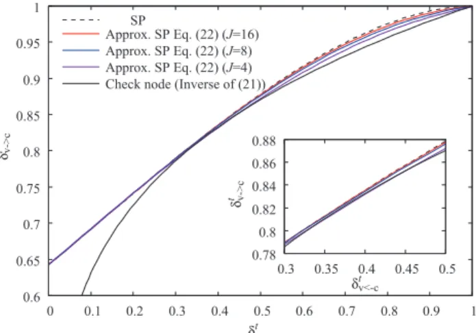
The DE equations (21) and (22) are numerically evaluated for the ensemble of (3,6)-regular LDPC codes. Figure 1 shows the chart of the D-domain parametersδvt→candδtv←c. We find that the curve of the approximate SP decoding gets closer to that of the exact SP decoding asJgrows. The error due to the polynomial approximation is large in the upper- right region while it is negligibly small in the lower-left region.
When the two curves for the variable and check nodes have a unique intersection, the performance of SP decoding converges to the intersection. In particular, the exact SP decoding converges to the point (1,1), which indicates no bit errors in the limit N → ∞. We refer to the infimum of the SNREb/N0 such that the two curves have a unique intersection as decoding threshold. Only when the SNR is above the decoding threshold, the exact SP decoding can
Fig. 1 Chart of the D-domain parameters forEb/N0=1.25 dB.
correct all errors as N→ ∞. From Fig. 1, we find that only the approximate SP decoding with J = 4 has a decoding threshold larger than 1.25 dB.
Table 1 lists the decoding threshold of the exact and approximate SP decoding algorithms based on the DE-GA.
The approximate SP decoding achieves the same threshold as the exact SP decoding whenJis at most 8. The decoding threshold of the approximate SP decoding with J = 16 is slightly smaller than that of the exact one. This observation should be regarded as an approximation error of the DE-GA.
We next investigate the impact of the position at which the channel message Dnis processed in the update rule (8) withF2 in (11) replaced byθ(F˜2J(D1,D2)). The DE equa- tions of the variable nodes are given by (22) and (23), respec- tively, when Dn is processed at the first and last positions.
Figure 2 shows a comparison between the two approximate SP decoding algorithms. When Dnis processed at the last position, the intersection between the two curves moves from the point(1,1)toward the lower-left direction. This implies that the channel messageDnshould be processed at the first position to improve the decoding performance after conver- gence.
This observation can be understood as follows: Suppose that the messages{Dtn←m0}emitted from all check nodes con- nected to variable nodenare 1. In the exact SP decoding, F2(Dtn←m0,Dn) =1 given in (7) holds regardless ofDn. In the approximate SP decoding, on the other hand, we find F˜2J(Dtn←m0,Dn) = (1+Dn)PJ
j=0(−Dn)j ∈ [0,1) for all Dn ∈[−1,0). In other words, the exact SP decoding trusts any message with magnitude 1 completely, while the approx- imate SP decoding still doubts if another message with the opposite sign is passed. When Dn < 0 is processed at the first position, the message emitted from variable node nis
Table 1 Decoding threshold based on the DE-GA.
SP Approx. SP Approx. SP Approx. SP (J=16) (J=8) (J=4)
1.20 dB 1.19 dB 1.20 dB 1.28 dB
Fig. 2 Chart of the D-domain parameters forEb/N0=1.25 dB.J=16 was used for the approximate SP decoding.
equal to 1. WhenDn <0 is processed at the last position, on the other hand, it is smaller than 1.
This discussion assumes that messages passed from check nodes are reliable. The assumption is valid in the limit N → ∞, as long as a finite number of iterations are considered. However, the messages may not be reliable for finite code length, because of the existence of short cycles in LDPC codes. Since it is overconfident in reliability of the messages, the exact SP decoding causes an error floor more likely than the approximate SP decoding.
5. Numerical Simulations
5.1 Performance
The performance of SP decoding is numerically investigated for the ensemble of(3,6)-regular LDPC codes. In all numer- ical simulations, the number of iterations is set to 50. We consider three decoding algorithms: the exact SP decoding in the D-domain, the approximate SP decoding, and the NMS decoding[16]. The exact SP decoding in the D-domain is equivalent to that in the L-domain. In the NMS decoding, the update rule (5) of the check nodes in the L-domain is replaced by
Ltn←m=α Y
n0∈Nm\ {n}
sign(Ltn0→m) min
n0∈Nm\ {n}{|Ltn0→m|}, (24) where the function sign(L) denotes the sign of L. The coefficientα > 0 is a design parameter for optimizing the performance of the NMS decoding. In this paper, we use α =0.8[16]optimized in terms of the decoding threshold for the ensemble of(3,6)-regular LDPC codes.
Figure 3 shows the BERs of the approximate SP de- coding with degrees J = 8 and J = 16 in (13) for short code lengthN =1024. The approximate SP decoding with J =16 achieves almost the same BER as the exact SP de- coding. As shown in[16], the NMS decoding is slightly superior to the SP decoding in the moderate SNR regime.
Fig. 3 BER versusEb/N0for code lengthN=1024.
However, the NMS decoding has the worst performance in the high SNR regime.
To understand what occurs in the high SNR regime, we show the BERs versus the number of iterations at a high SNR in Fig. 4. The BERs of the exact SP and NMS decoding oscillates as the number of iterations increases. The NMS decoding has worse convergence property than the exact SP decoding. This bad convergence properties are due to the existence of short cycles in LDPC codes. Since it is ex- perimentally known that optimizing the decoding threshold degrades the error-floor performance, the NMS decoding is more strongly affected by short cycles.
On the other hand, the BERs of the approximate SP decoding are monotonically decreasing in spite of the ex- istence of short cycles. This is because the approximate SP decoding is not overconfident in reliability of messages, as discussed at the end of Sect. 4. Thus, we can conclude that the approximate SP decoding improves the convergence property in the high SNR regime.
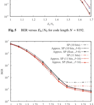
Figure 5 shows the BERs for long code length N = 8192. As reported in[16], the NMS decoding has a perfor- mance loss of approximately 0.05 dB compared to the exact SP decoding. The BER of the approximate SP decoding with J = 32 is indistinguishable from that of the exact SP decoding, while usingJ=16 results in a slight performance loss.
Finally, we investigate the influence of quantization.
As discussed in Sect. 3, we used the Q-bit signed fixed- point number representation of the interval [−2,2)based on the uniform quantization for the approximate SP decoding.
On the other hand, we used the same representation of the interval [−1,1)for the exact SP decoding in the D-domain.
Quantization of the NMS decoding is not considered since it requires the optimization of the quantization step for each number of quantization bits via DE[16].
Figure 6 shows the BERs of the exact and approximate SP decoding using the fixed-point number representation.
An interesting observation is that the quantization degrades significantly the performance of the exact SP decoding in the
Fig. 4 BER versus the number of iterations for code lengthN =1024 andEb/N0=3 dB.
Fig. 5 BER versusEb/N0for code lengthN=8192.
Fig. 6 BER versusEb/N0for code lengthN=1024.
high SNR regime. On the other hand, the approximate SP decoding achieves almost the same performance as the exact SP decoding with a double-precision floating-point number representation. Thus, we conclude that the approximate SP decoding is robust against the quantization errors.
5.2 Complexity
We compare the exact and approximate SP decoding algo- rithms in the D-domain in terms of resources and processing time in implementing them with an FPGA. As a fair com- parison, we focus on the update rules of each variable node instead of implementing the whole decoders. We used Cy- clone V SX SoCs 5CSXC6 produced by Intel Corporation to make modules implementing the update rules.
As long as LUTs are utilized, there are no essential differences between implementations of the two decoding algorithms. From the numerical simulations in Sect. 5.1, we can conclude that, when LUTs are used, the approx- imate SP decoding achieves robuster performance against quantization errors than the exact SP decoding in spite of comparable resources and processing time. Thus, we only compare implementations based on arithmetic operations.
Table 2 Resources and processing time per variable node. The values in the parentheses are for the DSP-enabled case.
ALMs Fmax[MHz] Proc. time [ns]
Approx. SP
(10 bits,J=8) 163 (96) 126 (141) 48 (43) SP (10 bits) 255 (206) 25 (24) 120 (125) Approx. SP
(11 bits,J=16) 189 (111) 115 (136) 61 (52) SP (11 bits) 303 (246) 20 (22) 148 (135)
We used the LPM_DIVIDE IP core to implement a divider, while we utilized the LPM_MULT IP core for a multiplier. TimeQuest Timing Analyzer in Intel Quartus Prime Lite Edition Software was used to estimate the number of adaptive logic modules (ALMs), the maximum operating frequency Fmax, and the processing time. The number of ALMs is regarded as the amount of resources required for implementing the modules.
Table 2 lists the number of ALMs, the maximum op- erating frequency, and the processing time for the exact and approximate SP decoding. Note that they depend on whether digital signal processing (DSP) is enabled or disabled. In the DSP-disabled case for J =16, the approximate SP de- coding reduces the amount of resources and the processing time by 38% and 59%, respectively, compared to the exact SP decoding.
6. Conclusion
We have proposed the SP decoding in the D-domain and an polynomial approximation of its update rule in each variable node. Use of the D-domain results in a simple implementa- tion of the decoder with a fixed-point number representation based on uniform quantization of a fixed interval. The inter- val does not depend on the ensemble of LDPC codes or the channel, in contrast to the NMS decoding that requires the optimization of design parameters via DE.
The approximate SP decoding in the D-domain has the following advantages:
1. It achieves almost the same performance as the exact SP decoding when an appropriate degree in the polynomial approximation is used.
2. It has better convergence property in the high SNR regime than the exact SP and NMS decoding.
3. It is robust against quantization errors.
4. It provides a significant reduction of resources and pro- cessing time compared to the exact SP decoding in the D-domain when it is implemented with arithmetic op- erations.
An important future work is to reduce the number of quantization bits. A possible approach is non-uniform quantization based on the maximization of mutual informa- tion[21]. The D-domain [−1,1] should be more suitable for such optimization than the L-domain(−∞,∞).
Acknowledgments
The authors thank anonymous reviewers for their sugges- tions that have improved the quality of the manuscript.
K. Takeuchi was in part supported by the Grant-in-Aid for Scientific Research (B) (JSPS KAKENHI Grant Number 18H01441), Japan.
References
[1] F.R. Kschischang, B.J. Frey, and H.A. Loeliger, “Factor graphs and the sum-product algorithm,” IEEE Trans. Inf. Theory, vol.47, no.2, pp.498–519, Feb. 2001.
[2] T. Richardson and R. Urbanke, Modern Coding Theory, Cambridge University Press, New York, 2008.
[3] S.Y. Chung, G.D. Forney, Jr., T.J. Richardson, and R. Urbanke, “On the design of low-density parity-check codes within 0.0045 dB of the Shannon limit,” IEEE Commun. Lett., vol.5, no.2, pp.58–60, Feb.
2001.
[4] S. Kudekar, T. Richardson, and R.L. Urbanke, “Spatially coupled ensembles universally achieve capacity under belief propagation,”
IEEE Trans. Inf. Theory, vol.59, no.12, pp.7761–7813, Dec. 2013.
[5] P. Hailes, L. Xu, R.G. Maunder, B.M. Al-Hashimi, and L. Hanzo, “A survey of FPGA-based LDPC decoders,” IEEE Commun. Surveys Tuts., vol.18, no.2, pp.1098–1122, Secondquarter 2016.
[6] Y. Chen and D. Hocevar, “A FPGA and ASIC implementation of rate 1/2, 8088-b irregular low density parity check decoder,” Proc.
2003 IEEE Global Commun. Conf., pp.113–117, San Francisco, CA, USA, Dec. 2003.
[7] Z. Cui and Z. Wang, “A 170 Mbps (8176, 7156) quasi-cyclic LDPC decoder implementation with FPGA,” Proc. 2006 IEEE Int. Symp.
Circuits Syst., pp.5095–5098, Island of Kos, Greece, May 2006.
[8] N. Chen, Y. Dai, and Z. Yan, “Partly parallel overlapped sum-product decoder architectures for quasi-cyclic LDPC codes,” Proc. 2006 IEEE Workshop Signal Process. Syst. Design Implement., pp.220–225, Banff, Canada, Oct. 2006.
[9] N. Wiberg, Codes and Decoding on General Graphs, Ph.D. thesis, Linköping Univ., Linköping, Sweden, 1996.
[10] M. Karkooti and J.R. Cavallaro, “Semi-parallel reconfigurable archi- tectures for real-time LDPC decoding,” Proc. Int. Conf. Inf. Technol.
Coding Comput., pp.579–585, Las Vegas, NV, USA, April 2004.
[11] L. Yang, H. Liu, and C.J.R. Shi, “Code construction and FPGA im- plementation of a low-error-floor multi-rate low-density parity-check code decoder,” IEEE Trans. Circuits Syst. I, Reg. Papers, vol.53, no.4, pp.892–904, April 2006.
[12] A. Darabiha, A.C. Carusone, and F.R. Kschischang, “A bit-serial approximate min-sum LDPC decoder and FPGA implementation,”
Proc. 2006 IEEE Int. Symp. Circuits Syst., pp.149–152, Island of Kos, Greece, May 2006.
[13] C. Beuschel and H.J. Pfleiderer, “FPGA implementation of a flexible decoder for long LDPC codes,” Proc. 2008 Int. Conf. Field Program.
Logic Appl., pp.185–190, Heidelberg, Germany, Sept. 2008.
[14] Y. Dai, Z. Yan, and N. Chen, “Optimal overlapped message passing decoding of quasi-cyclic LDPC codes,” IEEE Trans. Very Large Scale Integr. (VLSI) Syst., vol.16, no.5, pp.565–578, May 2008.
[15] X. Chen, J. Kang, S. Lin, and V. Akella, “Memory system optimiza- tion for FPGA-based implementation of quasi-cyclic LDPC codes decoders,” IEEE Trans. Circuits Syst. I, Reg. Papers, vol.58, no.1, pp.98–111, Jan. 2011.
[16] J. Chen, A. Dholakia, E. Eleftheriou, M.P.C. Fossorier, and X.Y.
Hu, “Reduced-complexity decoding of LDPC codes,” IEEE Trans.
Commun., vol.53, no.8, pp.1288–1299, Aug. 2005.
[17] T.J. Richardson and R.L. Urbanke, “The capacity of low-density parity-check codes under message-passing decoding,” IEEE Trans.
Inf. Theory, vol.47, no.2, pp.599–618, Feb. 2001.
[18] S.Y. Chung, T.J. Richardson, and R.L. Urbanke, “Analysis of sum- product decoding of low-density parity-check codes using a Gaussian approximation,” IEEE Trans. Inf. Theory, vol.47, no.2, pp.657–670, Feb. 2001.
[19] J. Boutros and G. Caire, “Iterative multiuser joint decoding: Unified framework and asymptotic analysis,” IEEE Trans. Inf. Theory, vol.48, no.7, pp.1772–1793, July 2002.
[20] S. ten Brink, “Convergence behavior of iteratively decoded par- allel concatenated codes,” IEEE Trans. Commun., vol.49, no.10, pp.1727–1737, Oct. 2001.
[21] F.J.C. Romero and B.M. Kurkoski, “LDPC decoding mappings that maximize mutual information,” IEEE J. Sel. Areas Commun., vol.34, no.9, pp.2391–2401, Sept. 2016.
Mizuki Yamada received the B. Eng. and M. Eng. from Toyohashi University of Technol- ogy, Aichi, Japan, in 2017 and 2019, respec- tively. He is currently an engineer at Sharp Cor- poration, where he works on the development of mobile communication systems.
Keigo Takeuchi received the B. Eng., M. Inf., and Ph.D. degrees in informatics from Kyoto University, Kyoto, Japan, in 2004, 2006, and 2009, respectively. From 2009 to 2016, he was an Assistant Professor at Department of Communication Engineering and Informatics, University of Electro-Communications, Japan.
He is currently an Associate Professor at De- partment of Electrical and Electronic Informa- tion Engineering, Toyohashi University of Tech- nology, Japan. He served as an Associate Editor of IEICE Trans. Fundamentals. from 2013 to 2017. He held visiting ap- pointments at Norwegian University of Science and Technology (NTNU), Norway, and at National Sun Yat-sen University (NSYSU), Taiwan. His re- search interests are in the field of wireless communications, statistical signal processing, and statistical-mechanical informatics. Dr. Takeuchi received the 2008 IEEE Kansai Section Student Paper Award and the IEEE Nagoya Section Young Researcher Awards 2017.
Kiyoyuki Koike was born in Tokyo, Japan on February 15, 1960. He received the B. Eng., M. Eng. and Ph.D. degrees in Electrical Engi- neering from Nagaoka University of Technology in 1982, 1984 and 2002, respectively. From 1984 to 1986, he was an engineer at Fujitsu Limited, where he worked on the development of super- visory circuit of submarine optical repeater and researched jitter accumulation. From 1986 to 1996, he was a research engineer at Sharp Cor- poration, where he worked on the development of mobile communication systems. From 1996 to 1999 he worked in the Nagaoka University of Technology. In 1999 he joined the Tokyo National College of Technology and he is now Professor in the Department of Elec- tronic Engineering. His current research interests include communication engineering, coding theory and embedded systems.