On the turning point problem for

RIMS-1693

On the turning point problem for

instanton-type solutions of Painlev´ e equations

By

Yoshitsugu TAKEI

April 2010

R _ESEARCH I NSTITUTE FOR M ATHEMATICAL S _CIENCES

On the turning point problem for

instanton-type solutions of Painlev´e equations

Yoshitsugu Takei

^∗

Research Institute for Mathematical Sciences Kyoto University, Kyoto 606-8502, Japan

[email protected]

Abstract

The turning point problems for instanton-type solutions of Painlev´e equations with a large parameter are discussed. Generalizing the main result of [KT2] near a simple turning point, we report in this paper that Painlev´e equations can be transformed to the second Painlev´e equation and the most degenerate third Painlev´e equation near a dou- ble turning point and near a simple pole, respectively. An outline of the proof based on the theory of isomonodromic deformations of associated linear differential equations is also explained.

1 Background and main results

The purpose of this report is to discuss the turning point problem for instanton-type solutions of Painlev´e equations from the viewpoint of exact WKB analysis.

In our series of papers ([KT1],[AKT],[KT2]) we develop the exact WKB analysis of Painlev´e equations (PJ) with a large parameter η (>0):

(PJ) d²λ

dt² =GJ

λ,dλ

dt, t

+η²FJ(λ, t).

∗Supported in part by JSPS Grants-in-Aid No. 20340028 and No. 21340029.

Here J runs over the following set of indices

(1.1) I ={I, II,III⁰, III⁰(D7), III⁰(D8), IV, V, VI},

and F_J(λ, t) andG_J(λ, µ, t) are some rational functions of (λ, t) and (λ, µ, t), respectively. For the concrete form of FJ(λ, t) and GJ(λ, µ, t) see Table 1 below. Note that instead of the usual third Painlev´e equation (PIII) we use (P_III⁰), which is equivalent to (P_III), for the sake of convenience in this paper. Note also that it is now considered to be natural to distinguish the degenerate third Painlev´e equations of type (D7) and (D8) from the generic third Painlev´e equation since the type of their affine Weyl group symmetries is different from that of the generic third Painlev´e equation. In this paper, being conformed to this convention, we have listed up (PIII⁰(D7)) and (PIII⁰(D8)) as well in Table 1. These Painlev´e equations (P_J) are related to one another according to the so-called coalescence diagram described in Table 2.

As can be readily confirmed, every Painlev´e equation (PJ) (J ∈ I) admits the following formal power series solution (in η⁻¹) called a “0-parameter solution”:

(1.2) λ⁽⁰⁾_J (t, η) =λ0(t) +η⁻²λ2(t) +η⁻⁴λ4(t) +· · · , where the top term λ0(t) satisfies an algebraic equation

(1.3) FJ(λ0(t), t) = 0

and the other terms λ_2j(t) (j ≥ 1) are recursively determined once λ₀(t) is fixed. Furthermore, by using the multiple-scale method, we have constructed in [AKT] the following formal solution of (PJ), called a “2-parameter solu- tion” or an “instanton-type solution”, containing 2 free complex parameters (α, β):

(1.4) λJ(t, η;α, β) =λ0(t) +η^−1/2λ1/2(t, η) +η⁻¹λ1(t, η) +· · · .

Here the leading termλ₀(t) is the same as that of a 0-parameter solution and the other terms λj/2(t, η) (j ≥1) are of the form

(1.5) λj/2(t, η) = Xj

k=0

b^(j/2)_j−2k(t) exp ((j−2k)ΦJ),

(P_I) d²λ

dt² = η²(6λ²+t).

(PII) d²λ

dt² = η²(2λ³+tλ+c).

(PIII⁰) d²λ dt² = 1

λ dλ

dt 2

− 1 t

dλ dt +η²

c∞λ³

t² − c⁰_∞λ² t² +c⁰₀

t −c₀ λ

.

(PIII⁰(D7)) d²λ dt² = 1

λ dλ

dt 2

− 1 t

dλ dt −η²

2λ² t² +c

t + 1 λ

.

(PIII⁰(D8)) d²λ dt² = 1

λ dλ

dt 2

− 1 t

dλ dt +η²

λ² t² −1

t

.

(PIV) d²λ dt² = 1

2λ dλ

dt 2

− 2 λ +η²

3

2λ³+ 4tλ²+ 2t²+c1

λ−c0

λ

.

(PV) d²λ dt² =

1

2λ + 1 λ−1

dλ dt

2

− 1 t

dλ

dt +(λ−1)² t²

2λ− 1 2λ

+η²2λ(λ−1)² t²

c∞− c0

λ² − c2t

(λ−1)² − c1t²(λ+ 1) (λ−1)³

.

(P_VI) d²λ dt² = 1

2 1

λ + 1

λ−1+ 1 λ−t

dλ dt

2

− 1

t + 1

t−1 + 1 λ−t

dλ dt +2λ(λ−1)(λ−t)

t²(t−1)²

1− λ²−2tλ+t 4λ²(λ−1)² +η²

c∞− c0t

λ² +c1(t−1)

(λ−1)² − ctt(t−1) (λ−t)²

.

Table 1: Painlev´e equations with a large parameter η. Here λ denotes an unknown function, t is an independent variable and c, c0 etc. are complex parameters.

(PVI) −→ (PV) −→ (PIII⁰) −→ (PIII⁰(D7)) −→ (PIII⁰(D8))

& &

(PIV) −→ (PII) −→ (PI) Table 2: Coalescence diagram of Painlev´e equations.

where ΦJ = ΦJ(t, η), sometimes called an “instanton”, is defined by (1.6) ΦJ(t, η) =η

Z tr

∂FJ

∂λ (λ0(s), s)ds+αβlog η²θJ(t)

with an appropriately defined functionθJ(t) andb^(j/2)_l (t) (l =j, j−2, . . . ,−j) are functions of t depending also on α and β but not on η, that is, the η- dependence of λ_j/2(t, η) comes only from the l-instanton terms exp(lΦ_J). In particular, the subleading term λ1/2(t, η) is of the form

(1.7) λ1/2(t, η) =µJ(t) (αexp(ΦJ) +βexp(−ΦJ)).

For the explicit forms of θJ(t) and µJ(t) we refer the reader to [KT2, Sec- tion 1].

The subject of our series of papers ([KT1],[AKT],[KT2]) is the analysis of the structure of λ⁽⁰⁾_J (t, η) and λJ(t, η;α, β) near a simple turning point of (PJ). Here a (simple) turning point of (PJ) is defined as follows:

Definition 1.1. Let d²

dt²∆λ=η²∂FJ

∂λ (λ⁽⁰⁾_J , t)∆λ (∆PJ)

+∂GJ

∂λ λ⁽⁰⁾_J ,dλ⁽⁰⁾_J dt , t

!

∆λ+ ∂GJ

∂µ λ⁽⁰⁾_J ,dλ⁽⁰⁾_J dt , t

! d dt∆λ be the linearized equation (or the Frech´et derivative) of (PJ) at its 0- parameter solution λ⁽⁰⁾_J . Then a turning point of (PJ) is, by definition, a turning point of (∆PJ). That is, a turning point of (PJ) is a zero of (∂FJ/∂λ)(λ0(t), t). In particular, a point t satisfying

(1.8) ∂F_J

∂λ (λ0(t), t) = 0 and ∂²F_J

∂λ² (λ0(t), t)6= 0

is called a simple turning point. Similarly, a Stokes curve (PJ) is defined as a Stokes curve of (∆PJ), that is, a Stokes curve (PJ) is an integral curve of the direction field Imp

(∂FJ/∂λ)(λ0(t), t)dt = 0 emanating from a turning point.

The main result of [KT2] is then described in the following Theorem 1.2 (where we put e to the variables relevant to (PJ) to distinguish them from those relevant to the first Painlev´e equation (PI)).

Theorem 1.2. Let t˜= ˜t∗ be a simple turning point of (PJ) and σ˜ a point on a Stokes curve emanating from ˜t∗. Then there exists a neighborhood V˜ of

˜

σ so that every 2-parameter instanton-type solution ˜λJ(˜t, η; ˜α,β)˜ of (PJ) is formally transformed to a2-parameter instanton-type solutionλI(t, η;α, β)of (PI) in V˜. To be more specific, there exist a formal transformation t(˜t, η) of an independent variable and a formal transformationx(˜x,˜t, η)of an unknown function of the form

t(˜t, η) = X

j≥0

tj/2(˜t, η)η^−j/2, (1.9)

x(˜x,˜t, η) = X

j≥0

x_j/2(˜x,˜t, η)η^−j/2, (1.10)

where tj/2 andxj/2 are holomorphic in bothx˜and ˜t, that satisfy the following relation:

(1.11) x(˜λ_J(˜t, η; ˜α,β),˜ ˜t, η) = λ_I(t(˜t, η), η;α, β).

Theorem 1.2 implies that the first Painlev´e equation (PI) can be thought of as a canonical equation (or a normal form) near a simple turning point of Painlev´e equations (PJ). For instanton-type solutions of (PI) we have the following connection formula on its Stokes curve, say, on {argt = π} (cf.

[T1]):

β⁰ 2^2α0β0

Γ(2α⁰β⁰+ 1) = β 2^2αβ Γ(2αβ + 1), (1.12)

e^2iπα0β0 α⁰ 2^−2α0β0

Γ(−2α⁰β⁰ + 1) =e^2iπαβ α 2^−2αβ

Γ(−2αβ+ 1) −ie^4iπαβ, (1.13)

whereλI(t, η;α, β) (resp., λI(t, η;α⁰, β⁰)) is an instanton-type solution of (PI) in {argt < π} (resp., {argt > π}). In particular, the analytic continuation

across the Stokes curve {argt = π} of a 0-parameter solution λ⁽⁰⁾_I (t, η) = λI(t, η; 0,0) in {argt < π} is given by λI(t, η;−i/(2√

π),0) in {argt > π}. In view of Theorem 1.2 it is expected that the same connection formula as (1.12) and (1.13) should hold also for an instanton-type solution of (P_J) on its Stokes curve emanating from a simple turning point.

The aim of this report is to discuss some generalizations of Theorem 1.2.

Now, what kind of generalizations of Theorem 1.2 is possible? To consider possible generalizations of Theorem 1.2, we first briefly review a simpler case, that is, the case of second order linear ordinary differential equations

(1.14)

− d²

dx² +η²Q(x)

ψ = 0.

It is well-known that at a simple turning point Equation (1.14) can be trans- formed into the Airy equation (i.e., Equation (1.14) with Q(x) = x). In fact, such a transformation is constructed in the framework of exact WKB analysis as well (cf. [KT3, Chapter 2]) and Theorem 1.2 can be regarded as a nonlinear analogue of this result. For linear equations (1.14) several gen- eralizations of this result are also known. For example, at a double turning point (i.e., a double zero ofQ(x)) (1.14) can be transformed into the Weber equation (i.e., Equation (1.14) with Q(x) = x² +η⁻¹E with some constant E). Furthermore at a simple pole of Q(x) (1.14) is transformed into the Whittaker equation (i.e., Equation (1.14) with Q(x) = 1/x+η⁻²γ/x² with some constant γ). This fact means that a simple pole of Q(x) also plays a role of turning points for Equation (1.14) and in the framework of exact WKB analysis this fact is verified by Koike in [K].

In parallel to the case of linear equations (1.14) we are then able to consider some generalizations of Theorem 1.2 for Painlev´e equations, that is, generalizations to a transformation near a double turning point and that near a simple pole. First, near a double turning point, we can prove the following

Theorem 1.3. Near a double turning point every 2-parameter instanton- type solution of (PJ) is formally transformed to that of the following second Painlev´e equation (PII,deg) (in the same sense as in Theorem 1.2):

(PII,deg) d²λ

dt² =η²(2λ³+tλ+η⁻¹c).

Note that (PII,deg) is different from the ordinary second Painlev´e equation (PII) in that the parameterc is multiplied by η¹ in (PII,deg) (while it is mul- tiplied by η² in (PII)). Next, near a simple pole, we have

Theorem 1.4. Near a simple pole every2-parameter instanton-type solution of (PJ) is formally transformed to that of the most degenerate third Painlev´e equation (PIII⁰(D8)) (in the same sense as in Theorem 1.2).

Theorem 1.3 and Theorem 1.4 are the main results of this report. Their precise statements will be given below in Theorem 2.5 and Theorem 3.1, respectively. Theorem 1.3 has been announced also in [T2].

The plan of this report is as follows: In Section 2, after discussing the exact WKB theoretic structure of (PII,deg), we give the definition of a double turning point of (PJ) and explain an outline of the proof of Theorem 1.3. A key idea is to use the relationship between Painlev´e equations and the theory of isomonodromic deformations of the associated linear differential equations.

Then in Section 3 we review the discussion of [T2], that is, we consider the transformation near a simple pole in a way parallel to Section 2. The details will be discussed in our forthcoming paper(s).

Acknowledgment:

The author is deeply grateful to Professor Takashi Aoki for his great assistance in completing the proof of Proposition 2.4 and to Professor Tatsuya Koike for his kind help in drawing Figure 1. He expresses his sincere gratitude also to Professor Takahiro Kawai for the stimulating discussions with him.

2 Transformation near a double turning point

2.1 Exact WKB theoretic structure of (P

II,deg

)

In this section we consider transformation near a double turning point. We first investigate the exact WKB theoretic structure of the canonical equation

(PII,deg) d²λ

dt² =η²(2λ³+tλ+η⁻¹c).

As was explained in Section 1, the top term λ0 = λ0(t) of the 0-parameter solution

(2.1) λ⁽⁰⁾_II,deg(t, η) =λ0(t) +η⁻¹λ1(t) +η⁻²λ2(t) +· · ·

of (PII,deg) is determined by an algebraic equation

(2.2) FII,deg(λ0, t) = 2λ³₀+tλ0 =λ0(2λ²₀+t) = 0.

Among the solutions of (2.2) we pick up a solution of 2λ²₀+t= 0, i.e.,

(2.3) λ0(t) =

r

−t

2 or −

r

−t 2

! ,

when we consider a double turning point. Note that, as (PII,deg) contains an odd order term ηc (with respect to η), λ⁽⁰⁾_II,deg(t, η) also contains odd order terms λ₁(t), λ₃(t), . . . . Then, starting with this top term λ₀(t) given by (2.3), we can construct a 2-parameter instanton-type solution of (PII,deg) of the form

λII,deg(t, η;α, β) (2.4)

=λ0(t) +η^−1/2(6λ²₀+t)^−1/4 αexp(ΦII,deg) +βexp(−ΦII,deg) +· · · with

(2.5) ΦII,deg(t, η) =η Z t

0

q

6λ²₀+sds+ (2αβ +c/2) log η²(6λ²₀+t)³ by employing the multiple-scale method. (Since (PII,deg) contains an odd order term ηc, the form of the instanton ΦII,deg is slightly different from the general form (1.6) of ΦJ.)

The linearized equation of (PII,deg) at a 0-parameter solution (2.1) is given by

(∆PII,deg) d²

dt²∆λ =η²

6(λ⁽⁰⁾_II,deg)²+t

∆λ =η² −2t+O(η⁻¹)

∆λ.

Hence (PII,deg) has a unique turning point at t = 0. Note that this turning point t = 0 is also an algebraic branch point of the Riemann surface of λ0(t). The Stokes curves of (PII,deg), i.e., integral curves of the direction field Imp

6λ²₀+t dt = Im√

−2t dt = 0 emanating from the turning point t = 0, thus consist of the following three lines:

(2.6) {t∈C | argt=π+ 2nπ/3 (n∈Z)}.

It is expected that a Stokes phenomenon should be observed on each Stokes curve for instanton-type solutions λII,deg(t, η;α, β). To analyze the Stokes phenomenon, we make use of the well-known relationship between the Painlev´e equation and the theory of isomonodromic deformations of the associated linear differential equation (cf. [O],[JMU]). In the case of (PII,deg) the relationship is formulated as follows: Let (SLII,deg) and (DII,deg) be the following linear differential equations, respectively.

(SLII,deg)

− ∂²

∂x² +η²QII,deg

ψ = 0,

(DII,deg) ∂ψ

∂t =AII,deg

∂ψ

∂x − 1 2

∂AII,deg

∂x ψ, where

Q_II,deg =x⁴+tx²+ 2η⁻¹cx+ 2K_II,deg−η⁻¹ ν

x−λ +η⁻² 3 4(x−λ)², (2.7)

AII,deg = 1 2(x−λ), (2.8)

with

(2.9) KII,deg = 1

2

ν²−(λ⁴+tλ²+ 2η⁻¹cλ) .

Then the compatibility condition of (SLII,deg) and (DII,deg) is represented by the Hamiltonian system

(HII,deg) dλ

dt =η∂K_II,deg

∂ν , dν

dt =−η∂K_II,deg

∂λ ,

which is equivalent to the second order differential equation (PII,deg) for λ.

As its consequence, we find that the monodromy data of (SLII,deg) should be independent of the deformation parameter t if a solution of (HII,deg) or (PII,deg) is substituted into the coefficients of (SLII,deg).

To determine the connection formula which describes the Stokes phe- nomenon forλII,deg(t, η;α, β) on a Stokes curve of (PII,deg), we then substitute λII,deg(t, η;α, β) into the coefficients of (SLII,deg) and compute its monodromy data by employing the exact WKB analysis. The following is a key proposi- tion in executing the computation of the monodromy data.

Proposition 2.1. If an instanton-type solution of (HII,deg) or (PII,deg) is substituted into the coefficients of (SLII,deg), the following hold:

(i) The top term(with respect to η⁻¹)Q0 of the potential QII,deg of (SLII,deg) is factorized as

(2.10) Q0 = (x−λ0(t))²(x+λ0(t))².

That is, (SL_II,deg) has two double turning points x=λ₀(t) and x=−λ₀(t).

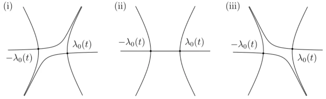
(ii) When t lies on a Stokes curve (2.6) of (PII,deg), there exists a Stokes curve of (SLII,deg) that connects the two double turning points x = ±λ0(t) of (SL_II,deg). (Cf. Figure 1, (ii), where the configuration of Stokes curves is shown when t lies on a Stokes curve argt =π.)

(i) (ii) (iii)

−λ₀(t)

λ₀(t) −λ₀(t) λ₀(t)

−λ₀(t)

λ₀(t)

Figure 1: Configuration of Stokes curves of (SL_II,deg) in the case of (i) argt <

π, (ii) argt =π, and (iii) argt > π.

Proposition 2.1, (ii) implies that a change of the configuration of Stokes curves of (SLII,deg) is observed on each Stokes curve of (PII,deg). For example, the change on a Stokes curve argt = π is visualized in Figure 1. This change of the configuration causes a Stokes phenomenon forλII,deg(t, η;α, β) to occur on a Stokes curve of (PII,deg). As a matter of fact, by substituting an instanton-type solution λ_II,deg(t, η;α, β) into the coefficients of (SL_II,deg) and employing the exact WKB analysis for linear equations, we obtain the following

Proposition 2.2. Suppose that an instanton-type solution of(P_II,deg)is sub- stituted into the coefficients of (SLII,deg). Let m^(±)₁ and m^(±)₂ be two indepen- dent monodromy data (i.e., Stokes multipliers around x=∞ in this case)of

(SLII,deg) when t belongs to the region Ω± = {t| ±(argt−π) >0}, respec- tively. Then (m^(±)₁ , m^(±)₂ ) can be explicitly computed as follows:

(When t∈Ω+)

m⁽⁺⁾₁ =−2√

π iβ 2^2αβ Γ(2αβ+ 1), (2.11)

m⁽⁺⁾₂ =−2√

π e^2iπαβ α 2^−2αβ Γ(−2αβ + 1). (2.12)

(When t∈Ω−) m⁽₁⁻⁾=−2√

π iβ 2^2αβ Γ(2αβ+ 1), (2.13)

m⁽⁻⁾₂ =−2√ π

e^2iπαβ α 2^−2αβ

Γ(−2αβ+ 1) −e^4iπαβ i 2^{c+2αβ−1/2} Γ(c+ 2αβ−1/2)

. (2.14)

Since the computation of monodromy data through the exact WKB analysis heavily depends on the configuration of Stokes curves, the concrete expres- sion of (m⁽⁺⁾₁ , m⁽⁺⁾₂ ) becomes different from that of (m⁽⁻⁾₁ , m⁽⁻⁾₂ ), as one can readily see in Proposition 2.2, due to the difference of two configurations of Stokes curves shown in Figure 1. On the other hand, thanks to the isomon- odromic property, the monodromy data should coincide if two instanton-type solutions in the two regions Ω± correspond to the same analytic solution.

Thus, if an instanton-type solutionλ_II,deg(t, η;α, β) in Ω− corresponds to the same analytic solution with λII,deg(t, η;α⁰, β⁰) in Ω+, we obtain the following relation in view of Proposition 2.2:

β⁰ 2^2α0β0

Γ(2α⁰β⁰+ 1) = β 2^2αβ Γ(2αβ+ 1), (2.15)

e^2iπα0β0 α⁰ 2^−2α0β0 Γ(−2α⁰β⁰+ 1) (2.16)

=e^2iπαβ α 2^−2αβ

Γ(−2αβ + 1)−e^4iπαβ i 2^{c+2αβ−1/2} Γ(c+ 2αβ−1/2).

In particular, the 0-parameter solutionλ⁽⁰⁾_II,deg(t, η) =λII,deg(t, η; 0,0) in the re- gion Ω−should be analytically continued toλII,deg(t, η;−i2^c−1/2/Γ(c+1/2),0)

in Ω+across the Stokes curve{argt =π}. This is the mechanism for a Stokes phenomenon to occur for instanton-type solutions of (PII,deg) on its Stokes curve. The above relations (2.15) and (2.16) describe the connection formula on {argt=π}.

2.2 Transformation theory to (P

II,deg

) near a double turning point

As we have observed in Subsection 2.1, in the case of (PII,deg) its linearized equation (∆PII,deg) has a unique turning point at t = 0 and three Stokes curves emanate from there. We call this kind of turning points a double turning point in general. To be more specific, we define a double turning point of (PJ) as follows:

Definition 2.3. A turning pointt =τd of (PJ) is said to be a double turning point if the following two conditions are satisfied.

(i) t=τ_d is an algebraic branch point of the Riemann surface of λ₀(t).

(ii) Near t=τd, (∂FJ/∂λ)(λ0(t), t) has a simple zero, that is,

(2.17) ∂FJ

∂λ (λ₀(t), t) = c(t−τ_d) +· · · holds with a non-zero constant c.

In particular, from each double turning point of (PJ) three Stokes curves emanate thanks to the condition (2.17). Note that at a simple turning point of (PJ) (∂FJ/∂λ)(λ0(t), t) has a square-root branch point (and hence the condition (i) is automatically satisfied there). Thus a double turning point is a turning point more degenerate than a simple turning point.

A Painlev´e equation (PJ) does not always have a double turning point.

For example, the first Painlev´e equation (PI) has a unique turning point at the origin t = 0 which is simple. Similarly, the degenerate third Painlev´e equation (PIII⁰(D7)) or (PIII⁰(D8)) does not possess any double turning point.

In order that (PJ) may have a double turning point, the parameters contained in (P_J) should satisfy some algebraic condition, the explicit form of which is described in the following

Proposition 2.4. (i) (PI), (PIII⁰(D7)) and (PIII⁰(D8)) have no double turning points.

(ii) A double turning point appears for a Painlev´e equation (PJ) (J =

II,III⁰,IV,V,VI) if and only if the parameters contained in (PJ) should sat- isfy the following relations:

c= 0 for J = II,

(2.18)

c0(c⁰_∞)²−c∞(c⁰₀)² = 0 for J = III⁰, (2.19)

2c0−c²₁ = 0 for J = IV, (2.20)

16c²₁c²∞−8c0c1c²₂−8c∞c1c²₂+c⁴₂ = 0 for J = V, (2.21)

16(c²₀c²₁+c²₁c²_t +c²_tc²₀)−32(c²₀c₁c_t+c₀c²₁c_t+c₀c₁c²_t) (2.22)

−64c0c1ct˜c∞−8(c0c1+c1ct +ctc0)˜c∞² + ˜c⁴∞= 0 for J = VI, where ˜c∞ =c∞−(c0+c1+ct) in the case of J = VI.

Throught this subsection we assume that the conditions (2.18) ∼ (2.22) listed in Proposition 2.4, (ii) are satisfied. The problem we want to discuss is to develop transformation theory near a double turning point. Let t = τd be a double turning point of (PJ) (J = II,III⁰,IV,V,VI). Generalizing the transformation theory (Theorem 1.2) near a simple turning point, we can then prove the following theorem which claims that every 2-parameter instanton-type solution of (PJ) is transformed to that of (PII,deg) near t = τd. (In stating Theorem 2.5, we put e to the variables relevant to (PJ) to distinguish them from those relevant to (PII,deg).)

Theorem 2.5. Suppose that the conditions (2.18)∼ (2.22)are satisfied. Let t˜= ˜τ_d be a double turning point of (P_J) (J = II,III⁰,IV,V,VI) and σ˜ be a point on a Stokes curve emanating from τ˜d. Then we can find a neighborhood V˜ of σ˜ and a formal power series of η⁻¹ with constant coefficients

(2.23) c(η) = c0+η⁻¹c1+η⁻²c2+· · ·

such that in V˜ every 2-parameter instanton-type solution λ˜J(˜t, η; ˜α,β)˜ of (PJ) is formally transformed to a 2-parameter instanton-type solution λ_II,deg(t, η;α, β) of the degenerate second Painlev´e equation

(2.24) d²λ

dt² =η²(2λ³+tλ+η⁻¹c(η))

with the infinite seriesc(η)of (2.23)being substituted into its coefficient. To be more specific, there exist a formal transformation t = t(˜t, η) of an inde- pendent variable and a formal transformation x = x(˜x,˜t, η) of an unknown

function of the form

t(˜t, η) = X

j≥0

η^−j/2tj/2(˜t, η), (2.25)

x(˜x,˜t, η) = X

j≥0

η^−j/2xj/2(˜x,˜t, η), (2.26)

where tj/2 andxj/2 are holomorphic in bothx˜and ˜t, that satisfy the following relation:

(2.27) x(˜λJ(˜t, η; ˜α,β),˜ ˜t, η) =λII,deg(t(˜t, η), η;α, β).

Hence the (degenerate) second Painlev´e equation (PII,deg) can be regarded as the canonical equation of Painlev´e equations near a double turning point.

Theorem 2.5 suggests that the connection formula (2.15) and (2.16) for (PII,deg) described in section 2.1 should hold also for an instanton-type solu- tion of (PJ) on its Stokes curve emanating from a double turning point.

Let us explain an outline of the construction of the transformationst(˜t, η) andx(˜x,˜t, η). It is done in a parallel way to the transformation theory near a simple turning point; we again make use of the relationship between Painlev´e equations and the theory of isomonodromic deformations of linear differential equations, that is, we use the fact that (PJ) is equivalent to the compatibility condition of a system of linear differential equations

(SLJ)

− ∂²

∂x² +η²QJ

ψ= 0,

(DJ) ∂ψ

∂t =AJ

∂ψ

∂x − 1 2

∂A_J

∂x ψ.

(See [KT1] or [KT3, Chapter 4] for the concrete form of QJ and AJ.) A key proposition in constructing the transformations is then the following Proposition 2.6, which is a generalization of Proposition 2.1 to (P_J).

Proposition 2.6. Suppose that the conditions (2.18) ∼ (2.22) are satisfied and let t=τd be a double turning point of (PJ) (J = II,III⁰,IV,V,VI). If an instanton-type solutionλJ(t, η;α, β)of(PJ)is substituted into the coefficients of (SLJ), then the following hold:

(i) The top term (with respect to η⁻¹) Q0 of the potential QJ of (SLJ) has

two double zeros, one of which is given by the top term λ0(t)of the instanton- type solution λJ(t, η;α, β). In what follows the other double zero is denoted by κ(t). Hence (SLJ) has two double turning points x=λ0(t) and x=κ(t).

(ii) When t lies on a Stokes curve of (PJ) emanating from a double turning pointt =τd, there exists a Stokes curve of(SLJ)that connects the two double turning points x=λ0(t) and x=κ(t) of (SLJ).

Using this Proposition 2.6 of geometric character, we construct the trans- formations in the following manner. (In what follows we again adopt the convention of putting e to the variables relevant to (PJ) and (SLJ) to dis- tinguish them from those relevant to (PII,deg) and (SLII,deg).) Let ˜t = ˜σ be a point on a Stokes curve of (PJ) emanating from a double turning point ˜t= ˜τd

and let ˜γ denote a Stokes curve of (SLJ) that connects the two double turn- ing points ˜x = ˜λ0(˜t) and ˜x = ˜κ(˜t) at ˜t = ˜σ (whose existence is guaranteed by Proposition 2.6, (ii)). Then we can construct an invertible formal trans- formation (x(˜x,˜t, η), t(˜t, η)) which brings the simultaneous equations (SLJ) and (DJ) into (SLII,deg) and (DII,deg) in a neighborhood of ˜γ× {σ˜}. That is, we have

Theorem 2.7. Under the above geometric situation there exist a neighbor- hood U˜ of the Stokes curve γ, a neighborhood˜ V˜ ofσ, and a formal coordinate˜ transformation

x=x(˜x,˜t, η) = X

j≥0

η^−j/2xj/2(˜x,t, η),˜ (2.28)

t=t(˜t, η) = X

j≥0

η^−j/2t_j/2(˜t, η) (2.29)

withxj/2(˜x,t, η)˜ andtj/2(˜t, η)being holomorphic onU˜×V˜ andV˜, respectively, for which the following conditions (i)∼ (v) are satisfied:

(i) The function x0(˜x,˜t, η) is independent of η and ∂x0/∂x˜ never vanishes on U˜ ×V˜.

(ii) The function t0(˜t, η) is also independent of η and dt0/d˜t never vanishes on V˜.

(iii) x0(˜x,˜t) and t0(˜t) satisfy

x0(˜λ0(˜t),t, η) =˜ λ0(t0(˜t)) = r

−t0(˜t) 2 , (2.30)

x0(˜κ0(˜t),t, η) =˜ −λ0(t0(˜t)) =− r

−t₀(˜t) 2 . (2.31)

(iv) x1/2 and t1/2 identically vanish.

(v) If ψ(x, t, η) is a WKB solution of (SLII,deg) that satisfies (DII,deg) also, then ψ(˜˜ x,˜t, η) defined by

(2.32) ψ(˜˜ x,˜t, η) =

∂x(˜x,t, η)˜

∂x˜

−1/2

ψ(x(˜x,˜t, η), t(˜t, η), η) satisfies both (SLJ) and (DJ) on U˜ ×V˜

The transformations (2.25) and (2.26) that provide a local equivalence (2.27) between ˜λJ(˜t, η; ˜α,β) and˜ λII,deg(t, η;α, β) in Theorem 2.5 are given by the semi-global transformation (2.28) and (2.29) constructed in Theorem 2.7.

Otherwise stated, by considering a transformation for the underlying system (SLJ) and (DJ) of linear differential equations, we can find a transformation of the Painlev´e equation (PJ). This is a sketch of the proof of Theorem 2.5.

The details will be discussed in our forthcoming paper.

3 Transformation near a simple pole

As was outlined in [T2], the transformation theory near a simple pole, i.e., Theorem 1.4, is proved in a parallel way to the case of the transformation theory near a double turning point discussed in Section 2. In this section we briefly review the discussion of [T2] to explain the transformation near a simple pole.

In view of the list of Painlev´e equations (Table 1) we readily find that the Painlev´e equations (PJ) have the following singular points:

(3.1)

(PI), (PII), (PIV) : {∞}, (PIII⁰), (PIII⁰(D7)), (PIII⁰(D8)), (PV) : {0,∞},

(PVI) : {0,1,∞}.

Among them a pair of a Painlev´e equation and its singular point contained in the following list is of “the first kind” or of “regular singular type”.

((PIII⁰),0), ((PIII⁰(D7)),0), ((PIII⁰(D8)),0), ((PV),0), ((PVI),0), ((PVI),1), ((PVI),∞).

(3.2)

At a singular point of the first kind, in addition to a double pole type 0- parameter solution, there exists a simple pole type 0-parameter solution,

that is, for any pair ((PJ), τs) in (3.2), there exists a 0-parameter solution whose top term λ0(t) has a branch point at t=τs and satisfies

(3.3) ∂FJ

∂λ (λ₀(t), t) =O((t−τ_s)^−3/2) as t→τ_s,

where FJ(λ, t) denotes the coefficient of η² in the expression of (PJ). Note that the condition (3.3) guarantees that the corresponding linearized equa- tion (∆PJ) of (PJ) at the 0-parameter solution in question has a simple pole type singularity at t = τs after a new independent variable ˜t = (t−τs)^1/2, which is a local parameter of the Riemann surface of λ0(t) at t = τs, is in- troduced. Consequently, if ((PJ), τs) is a simple pole, only one Stokes curve of (PJ) emanates from t =τs.

Using the top term λ0(t) of a simple pole type 0-parameter solution, we can also construct a 2-parameter instanton-type solution λJ(t, η;α, β) of simple pole type for each pair ((P_J), τ_s) listed in (3.3). The problem we want to discuss is then to develop transformation theory for these instanton-type solutions λJ(t, η;α, β) of simple pole type. The precise formulation of the main result (i.e., Theorem 1.4) in this case is the following theorem (where we again adopt the convention of putting e to the variables relevant to (PJ) to distinguish them from those relevant to (PIII⁰(D8))).

Theorem 3.1. Let λ˜J(˜t, η; ˜α,β)˜ be a 2-parameter instanton-type solution of simple pole type for one of the pairs ((PJ),τ˜s) of a Painlev´e equation and its singular point listed in (3.2). Let σ˜ be a point on a Stokes curve ema- nating from τ˜s. Then we can find a neighborhood V˜ of σ˜ and a 2-parameter instanton-type solution λIII⁰(D8)(t, η;α, β)of (PIII⁰(D8)) such that λ˜J(˜t, η; ˜α,β)˜ is formally transformed to λIII⁰(D8)(t, η;α, β)in V˜. To be more specific, there exist a formal transformation t = t(˜t, η) of an independent variable and a formal transformation x=x(˜x,˜t, η) of an unknown function of the form

t(˜t, η) = X

j≥0

η^−j/2tj/2(˜t, η), (3.4)

x(˜x,˜t, η) = X

j≥0

η^−j/2x_j/2(˜x,˜t, η), (3.5)

where tj/2 andxj/2 are holomorphic in bothx˜and ˜t, that satisfy the following relation:

(3.6) x(˜λJ(˜t, η; ˜α,β),˜ ˜t, η) = λIII⁰(D8)(t(˜t, η), η;α, β).

Thus (PIII⁰(D8)) can be thought of as a canonical equation of Painlev´e equa- tions near a simple pole.

The proof of Theorem 3.1 is done in a parallel way to that of Theorem 2.5.

We again make use of the fact that a Painlev´e equation (PJ) is equivalent to the compatibility condition of (SLJ) and (DJ) given in Section 2. A key geometric proposition in this case is the following

Proposition 3.2. Suppose that an instanton-type solution λJ(t, η;α, β) of simple pole type of (P_J) is substituted into the coefficients of (SL_J). Then the following hold:

(i) The top term (with respect to η⁻¹) Q0 of the potential QJ of (SLJ) has a double zero at x = λ0(t), that is, (SLJ) has a double turning point at x=λ0(t).

(ii) When t lies on a Stokes curve of(PJ)emanating from a simple pole type singular point τs in question, there exists a Stokes curve of (SLJ) that starts from λ0(t)and returns toλ0(t)after encircling several singular points and/or turning points of (SLJ).

For example, in the case of the canonical equation, i.e., the most degen- erate third Painlev´e equation (PIII⁰(D8)),

(3.7) λ⁽⁰⁾_III0(D8)(t, η) =√ t

is a 0-parameter solution and the linearized equation of (PIII⁰(D8)) at this 0-parameter solution is given by

(∆PIII⁰(D8)) d²

dt²∆λ =η² 2

t^3/2 −η⁻² 1 4t²

∆λ.

Hence t= 0 is a simple pole type singularity (and a unique turning point) of (PIII⁰(D8)) and only one Stokes curve

(3.8) {t ∈C | argt= 4nπ (n ∈Z)}

(i.e., the positive real axis) emanates fromt= 0. Since the potential Q_III⁰_(D8) of the associated linear equation (SLIII⁰(D8)) has the form

QIII⁰(D8) = t 2x³ + 1

2x+ λ² x²

ν²−

t 2λ³ + 1

2λ (3.9)

−η⁻¹λν 1

x² + 1 x(x−λ)

+η⁻² 3 4(x−λ)²

(where ν =η⁻¹(tdλ/dt+λ)/(2λ²)), its top term Q0(x, t) becomes

(3.10) Q0(x, t) = (x−√

t)² 2x³

after the substitution of an instanton-type solution of simple pole type of (PIII⁰(D8)) beginning with the leading termλ0(t) =√

t. Using (3.10), we thus find that when t lies on a Stokes curve of (PIII⁰(D8)), i.e., when t >0, a circle {|x|=√

t} is a Stokes curve of (SLIII⁰(D8)) that starts from√

t, encircles the simple pole t = 0, and returns to√

t, as is indicated in Figure 2, (ii).

(i) (ii) (iii)

0

√t

0

√t

0 √

t

Figure 2: Configuration of Stokes curves of (SLIII⁰(D8)) in the case of (i) argt >0, (ii) argt= 0, and (iii) argt <0.

In parallel to Theorem 2.7, near a Stokes curve γ of (SLJ) that starts from a double turning point λ0(t) and returns to λ0(t) at a point t = σ on a Stokes curve of (PJ) emanating from a simple pole whose existence is guaranteed by Proposition 3.2, (ii), we can construct an invertible formal transformation which brings (SLJ) and (DJ) into (SLIII⁰(D8)) and (DIII⁰(D8)) in a neighborhood of γ × {σ}. That is, we have

Theorem 3.3. Let((PJ),τ˜s)be one of the pairs in the list (3.2)and˜σa point on a Stokes curve emanating fromτ˜_s. Suppose that an instanton-type solution λ˜J(˜t, η; ˜α,β)˜ of simple pole type of (PJ) is substituted into the coefficients of (SLJ). Then there exist a neighborhoodU˜ of a Stokes curve ˜γ of (SLJ)that starts from and returns to λ˜₀(˜t) at ˜t = ˜σ, a neighborhood V˜ of σ, and a˜ formal coordinate transformation of the form

x=x(˜x,˜t, η) = X

j≥0

η^−j/2xj/2(˜x,t, η),˜ (3.11)

t=t(˜t, η) = X

j≥0

η^−j/2tj/2(˜t, η) (3.12)

withxj/2(˜x,˜t, η)andtj/2(˜t, η)being holomorphic onU˜×V˜ andV˜, respectively, for which the following conditions (i)∼ (v) are satisfied:

(i) The function x0(˜x,˜t, η) is independent of η and ∂x0/∂x˜ never vanishes on U˜ ×V˜.

(ii) The function t0(˜t, η) is also independent of η and dt0/d˜t never vanishes on V˜.

(iii) x0(˜x,˜t) and t0(˜t) satisfy

(3.13) x₀(˜λ₀(˜t),˜t, η) =λ₀(t₀(˜t)) = q

t₀(˜t).

(iv) x1/2 and t1/2 identically vanish.

(v) If ψ(x, t, η) is a WKB solution of (SL_III⁰_(D8)) that satisfies (D_III⁰_(D8)) also, then ψ(˜˜ x,t, η)˜ defined by

(3.14) ψ(˜˜ x,˜t, η) =

∂x(˜x,t, η)˜

∂x˜

−1/2

ψ(x(˜x,˜t, η), t(˜t, η), η) satisfies both (SL_J) and (D_J) on U˜ ×V˜.

The semi-global transformation (3.11) and (3.12) constructed in Theo- rem 3.3 again provides a local equivalence (3.6) between ˜λJ(˜t, η; ˜α,β) and˜ λIII⁰(D8)(t, η;α, β) in Theorem 3.1. This is a sketch of the proof of Theo- rem 3.1. The details will be discussed in our forthcoming paper.

In the case of the canonical equation (PIII⁰(D8)), we can explicitly compute the monodromy data of the associated linear equation (SLIII⁰(D8)) by using exact WKB analysis for linear differential equations. Combining this com- putation with Proposition 3.2, we obtain the following connection formula for instanton-type solutions of (PIII⁰(D8)) on its Stokes curve argt = 0: Let λ(t, η;α, β) and λ(t, η;α⁰, β⁰) be instanton-type solutions of (PIII⁰(D8)) in the region Ω− ={argt < 0} and Ω+ ={argt > 0}, respectively. If λ(t, η;α⁰, β⁰) is the analytic continuation of λ(t, η;α, β) across the Stokes curve argt= 0, then we have

α⁰ 2^−2α0β0

Γ(−2α⁰β⁰+ 1) = α 2^−2αβ Γ(−2αβ+ 1), (3.15)

iβ⁰ 2^2α0β0

Γ(2α⁰β⁰+ 1) +e^2iπα0β0 α⁰ 2^−2α0β0 Γ(−2α⁰β⁰+ 1) (3.16)

= iβ 2^2αβ

Γ(2αβ+ 1) −e^−2iπαβ α 2^−2αβ Γ(−2αβ + 1).

See [TW, Section 5] for the computation of the monodromy data of (SLIII⁰(D8)). Theorem 3.1 then suggests that the same connection formula as (3.15) and (3.16) should hold also for instanton-type solutions of simple pole type of (PJ) listed in (3.2) on its Stokes curve emanating from a simple pole.

References

[AKT] Aoki, T., Kawai, T. and Takei, Y., WKB analysis of Painlev´e tran- scendents with a large parameter. II,Structure of Solutions of Dif- ferential Equations, World Scientific Publishing, 1996, pp. 1–49.

[JMU] Jimbo, M., Miwa, T. and Ueno, K., Monodromy preserving defor- mation of linear ordinary differential equations with rational coeffi- cients. I, Phys. D, 2 (1981), 306–352.

[KT1] Kawai, T. and Takei, Y., WKB analysis of Painlev´e transcendents with a large parameter. I, Adv. Math., 118 (1996), 1–33.

[KT2] , WKB analysis of Painlev´e transcendents with a large pa- rameter. III,Adv. Math., 134 (1998), 178–218.

[KT3] , Algebraic Analysis of Singular Perturbation Theory, AMS, 2005.

[K] Koike, T., On the exact WKB analysis of second order linear ordi- nary differential equations with simple poles,Publ. Res. Inst. Math.

Sci., 36 (2000), 297–319.

[OKSO] Ohyama, Y., Kawamuko, H., Sakai, H. and Okamoto, K., Studies on the Painlev´e equations. V,J. Math. Sci. Univ. Tokyo,13(2006), 145–204.

[O] Okamoto, K., Isomonodromic deformation and Painlev´e equations, and the Garnier systems, J. Fac. Sci. Univ. Tokyo, Sect. IA, 33 (1986), 575–618.

[T1] Takei, Y., An explicit description of the connection formula for the first Painlev´e equation, Toward the Exact WKB Analysis of Differ- ential Equations, Linear or Non-Linear, Kyoto Univ. Press, 2000, pp. 271–296.

[T2] , On the role of the degenerate third Painlev´e equation of type (D8) in the exact WKB analysis, preprint (RIMS-1660), 2009.

[TW] Takei, Y. and Wakako, H., Exact WKB analysis for the degenerate third Painlev´e equation of type (D8), Proc. Japan Acad., Ser. A, 83 (2007), 63–68.