1. Introduction
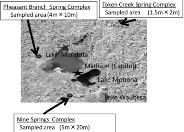
Many springs are distributed in the greater Madison area providing considerable portion of base flow to the lakes located in Yahara River basin in Wisconsin (Fig. 1).
Quality and quantity of the spring waters have significant effects on surface waters.
Groundwater as well as spring waters in the greater Madison area have been studied extensively mainly to access and construct a better water management plan to meet increasing water demands in the area. Decrease of spring flow rates and elevated nitrogen and chloride concentrations due to heavy agricultural activities and extensive urbanization in the watersheds are the major concern (Wisconsin Groundwater Advisory Committee, 2006, Institute for Environmental Studies University of Wisconsin-Madison, 1996, Dane County Regional Planning Commission, 1999).
Nitrogen and chloride generally enter subsurface system from recharge area with infiltrating precipitation. A part of the contaminants entered in the porous media is then transported to relatively small discharge zones. The gentle land relief and complex geology, however, make it difficult to delineate recharge and discharge areas in these watersheds. Bradbury and others (1999) illustrated a fairly complex recharge
Water chemistry characteristics of spring complexes near Madison, Wisconsin
SUGITA, Fumi
Figure 1 Location of study sites
and discharge area distribution for the Mt. Simon aquifer which was the major aquifer in the area. Hunt and others (2001) delineated a recharge area for the Pheasant branch springs using Monte Carlo approach with a numerical model. They found that capture zones are extending out of topographical watershed boundaries, which is commonly found in this area. Hunt and others (2001) also reported the gradational change in spring water chemistry which was attributed to bedrock geology.
In order to access the effects of human activities on spring waters and also on surface waters, it is important to identify the source areas and to understand the transport processes and the pathways between the source areas and the springs.
Spring water chemistry may indicate processes taking place during contaminant transport in its flow path.
High flow springs were sampled at discharging points and analyzed for pH, EC, DO, NO‑N, Cland alkalinity within three spring complexes located near Madison Wisconsin. The dimensions of the sampled areas in this study were 5m×20m for the Nine Springs, 4m×10m for Pheasant Branch and 1.5m×2m for Token Creek. The spatial chemistry distributions within the three spring complexes as well as correlations among chemical components were examined to evaluate degree of solute mixing in the flow paths. Numerical simulation was performed using HYDRUS 2D/3D (Simunek and others, 2007) to estimate mechanisms of mixing taking place in the flow paths.
2. Study sites and methods
2.1 Hydrogeology and climatology
The central to eastern part of Dane county in which Yahara River Basin locates is covered by relatively thick glacial deposits. The four lakes (L. Mendota, L. Monona, L. Waubesa and L. Kegonsa) and surrounding wetlands are formed on the glacial deposits.
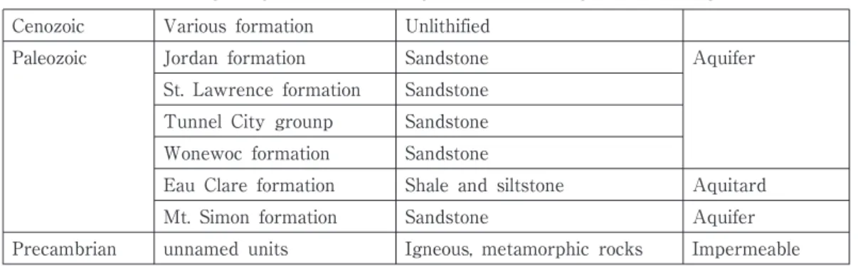
Hydrologically, four lumped units of stratifications (glacial unlithified deposits of Pleistocene, sandstone and dolomite aquifers of upper Paleozoic, a leaky confining aquitard called Eau Clair formation and sandstone formations called Mt. Simon aquifer) were identified on Precambrian bedrock (e.g. Bradbury, et.al., 1999, Swanson et al., 2001). The stratifications are summarized in Table 1.
Based on geochemical and isotope analysis of spring and groundwaters, Swanson and others (2001) identified three groups of different chemical characteristics. They indicated that majority of spring water travel through upper bedrock aquifer, while some travel through lower bed rock aquifer with longer travel time. The presence of layers that has high permeability (K) was also indicated in Tunnel city group which belongs to upper bed rock aquifer. It was suggested that these thin high permeable layers may play an important roll in groundwater flow and solute transport in this area (Swanson et al. 2006, Swanson and Bahr, 2004)
Madison area has typical continental North American climate. Annual monthly average temperature ranges from −8.2℃ (January) to 22℃ (July), with annual average temperature of 7.8℃. Approximately, 56% of precipitation fall during summer months (May to September), while winter months (December to February) are dry. A thirty year (1971‑2000) normal monthly precipitation and temperature (National Climate Data Center) at Madison WSO Airport station (station number 474961) is shown in Table 2.
2.2 Study sites
The three spring complexes in different watersheds near Madison were studied.
2.2.1 Nine Springs complex
Nine springs creek flows south of Madison area toward east and discharges into Yahara River between Lake Monona and Lake Waubesa (Fig. 1). The watershed (33m2) consists of mainly industrial and residential areas. Presence of number of spring complexes have been reported along the creek and studied extensively mainly to assess effects of municipal and industrial wells nearby (e.g. Inst. for Environ.
Studies, University of Wisconsin-Madison, 1996, Swanson and others, 2001). The spring complex examined in this study locates north-side of the creek in the middle of 9km-long creek. Fast flowing spring waters were sampled at 28 discharging points within 5m×10m stream bed (Photo 1).
Table 1 Stratigraphy of Dane County (based on Clayton and Attig, 1997)
Cenozoic Various formation Unlithified
Paleozoic Jordan formation Sandstone Aquifer
St. Lawrence formation Sandstone Tunnel City grounp Sandstone Wonewoc formation Sandstone
Eau Clare formation Shale and siltstone Aquitard
Mt. Simon formation Sandstone Aquifer
Precambrian unnamed units Igneous, metamorphic rocks Impermeable
Table 2 Monthly normal precipitations and temperature at Madison WAO Air port WI station (1971‑2000) (based on NCDC homepage, 2009)
Madison WAO Airport WI Station Number 474961 1971‑2000 monthly Normals
(National Climate Data Center 2009, units have been converted to SI units)
Month 1 2 3 4 5 6 7 8 9 10 11 12
P(mm) 31.6 32.4 57.7 84.3 83.3 102.5 94.8 109.5 77.9 55.2 58.4 42
T(℃) −8.2 −5.2 0.9 7.7 14.3 19.4 22 20.6 15.9 9.6 1.9 −5
2.2.2 Pheasant Branch spring complex
Pheasant Branch creek flows into Lake Mendota from north-west side (Fig. 1).
Its watershed (60km2) is agricultural dominated but mixture of developing urban area. The spring complex sampled in this study locates 1.5km north of lake shore.
The water from the spring complex generates a tributary of the Pheasant Branch creek and flows into the main stream approximately 800m downstream from the sampled area. Fast flowing spring waters were collected at 19 discharging points within 4m×10m area (Photo 2).
2.2.3 Token Creek spring complex
Token Creek is a tributary of Yahara River and flows into Lake Mendota from north-east side (Fig. 1). The watershed (220km2) consists of mainly agricultural area with increasing urban area (Lower Rock River Water Quality Management Plan, 2001). Numerous fast flow springs and seeps can be identified within and around the Token creek. The spring complex sampled in this study locates approximately 3km north-east of Cherokee marsh which is the last large wetland locates adjacent to the lakeshore. The spring waters were sampled at the 12 discharging points within 1.5m×2m portion of north upstream spring complex (Photo 3).
Photo 1 Nine Springs Photo 2 Pheasant Branch springs
Photo 3 Token Creek springs
2.3 Methods of sample collection and analysis
Spring waters were sampled at discharging points by placing a sampling tube in the fast flowing water and sealing it in the water in August and September of 2008.
High flow" point for sampling in this study was determined only by feeling of flowing water pressure on hands and also by observing boiling sands caused by flow pressure. However, all sampled points are estimated to have discharging rates more than 1.5 l/min from area of less than 0.1m2.
The water temperature and pH were measured on sites, while the rest of the chemical analysis was conducted in the laboratory at University of Wisconsin- Madison. All samples were analyzed for pH, EC (Hanna instruments, HI98130), DO, NO‑N, Cl and alkalinity (CHEMEtrics, Visual Analysis).
Numerical modeling was performed using HYDRUS2D/3D (Simunek and others, 2007).
3. Spring water chemistry
3.1 Averages and ranges of the solute concentrations
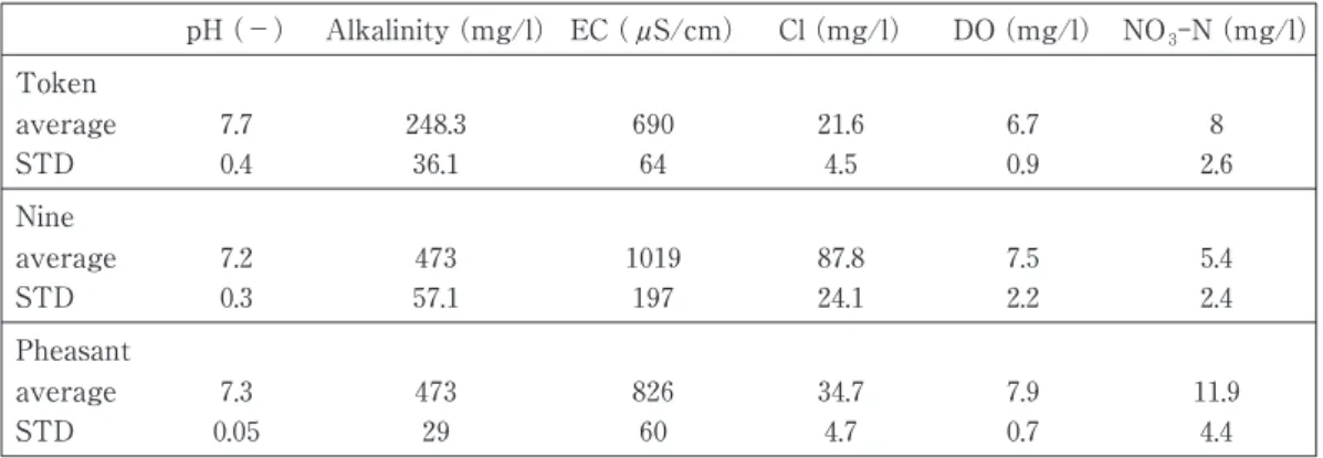
The results of spring water chemistry analysis are summarized in Table 3 and are shown in Figure 2.
An average pH values in the three spring complexes are close to 7 and have little variations (Fig. 2 (a)). Though agricultural point sources often generate low pH in groundwater, no indication of such point sources was found despite of heavy agricultural land use in Pheasant Branch and Token Creek watersheds. The pH values in Pheasant Branch have very narrow range with little standard deviation, indicating high buffering mechanism in the geology of the area. The major aquifer and flow paths in the study area consist of mainly sand stone and dolomite except undifferentiated unlithified glacial surface deposits. Both sand stone and dolomite are, in general, produce groundwater of low salinity and high HCOconcentration.
Table 3 Summary of spring water chemistry
pH (−) Alkalinity (mg/l) EC (μS/cm) Cl (mg/l) DO (mg/l) NO‑N (mg/l) Token
average 7.7 248.3 690 21.6 6.7 8
STD 0.4 36.1 64 4.5 0.9 2.6
Nine
average 7.2 473 1019 87.8 7.5 5.4
STD 0.3 57.1 197 24.1 2.2 2.4
Pheasant
average 7.3 473 826 34.7 7.9 11.9
STD 0.05 29 60 4.7 0.7 4.4
High average alkalinity values are found, in the three complexes (Fig. 2 (b)).
Alkalinity represents acid-neutralizing capacity of the porous medium (Stumm and Morgan, 1996). High alkalinity concentrations indicate that the groundwater is rich in HCO and therefore has a high capability of buffering acidic precipitation. The Ordovician carbonate rocks found in western part of Pheasant Branch watershed Figure 2 EC, pH and anion concentrations. Horizontal line in box is median.
Tops and bottoms of box represent 75th and 25th percentiles, respectively.
Vertical lines extend to 90th and 10th percentiles.
(a) pH (b) Alkalinity (c) Electric Conductivity (d) Chloride (e) Nitrate
(d) (e)
(a) (b) (c)
may be responsible for this extremely uniform pH values found in the spring waters.
Electrical conductivity (EC) indicates amount of total dissolved ions within the concentration range (less than 500meq/l) observed in this study (Mazor, 1991). Average EC value is very high (1019μS/cm) at Nine Springs suggesting high dissolved ion concentrations in the spring water (Table 3, Figure 2 (c)). The standard deviation of Nine Spring waters is also large (197μS/cm)). Both Pheasant Branch and Token Creek also show high average EC values (827μS/cm and 690μS/cm) compared those of natural springs (less than 100μS/cm) and surrounding surface waters (300‑
450μS/cm) .
Chloride (Cl) concentrations of the Nine springs are distinctively high (Table 3, Figure 2 (d)), indicating significant effects of urban land use (road salts) in the watershed. The standard variation of the chloride concentration is also large. Chloride is considered to be a conservative solute. The large standard variation in chloride concentrations in the spring waters, thus, suggests the presence of different flow regime within a single spring complex.
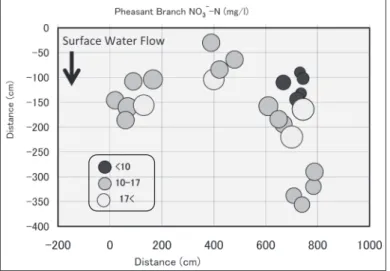
Nitrate (NO) concentrations at Pheasant Branch spring complexes are high and the average value exceeds the drinking water standard (10mg/l) (Table 3, Figure 2 (e)). The effect of agricultural activities in the area is obvious. Nitrate concentration tends to vary within a short distance due to degradation. However, high DO concentrations found in the water suggest that denitrification process is unlikely to take place in these waters. Thus, variation in nitrate concentrations may also indicate presence of different contributing source areas and different flow paths for the waters discharging into the same spring complex.
Dissolved oxygen (DO) concentrations in the three spring complexes are high for spring water (Table 3), indicating that the oxygen was not consumed along the flow paths. Major factor that determines DO concentrations of spring waters is the distance and time to travel from recharge area to the discharge area (Stumm and Morgan, 1996). Since confined groundwater usually have lost most or all its dissolve oxygen (Mazor, 1991), relatively high DO values observed indicate that the water did not flow through confined aquifer and that water is relatively young.
3.2 Anion composition and spatial concentration distribution within a single complex
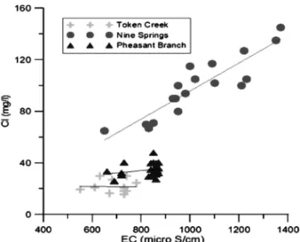
The relationships between EC and chloride concentrations are shown in Figure 3.
A clear positive correlation was observed only in concentrations of Nine Springs.
Since EC values directly indicate total dissolved ion concentrations, a positive correlation indicates that chloride is the major anion component in Nine Springs. A linear relationship is often generated by mixing two waters of different chloride concentrations. Therefore, it is suggested that two sources of chloride may be contributing to the small discharging area sampled in this study. No clear correlation
was found in concentrations in other two agricultural watersheds. However, the concentrations in Pheasant Branch show two distinct clusters (EC of around 500μS/
cm and 900μS/cm), suggesting presence of at least two different sources for these springs.
The spatial distribution of chloride concentrations within Nine Springs complex is shown in Figure 4. Large contrasts in concentrations were found within a few meters apart. No apparent trend with respect to space was observed.
The relationships between EC and nitrate are shown in Figure 5. A positive correlation is observed in concentrations from Pheasant Branch springs, indicating nitrate is the major anion component in Pheasant Branch springs. No correlation is
Figure 3 The relationship between EC and chloride concentrations
Figure 4 Distribution of chloride concentrations (mg/l) in Nine Springs complex
found in the concentrations of Token Creek or in those of Nine Springs. The EC values less than 800μS/cm in Nine Springs are almost linearly correlated to nitrate concentrations. The linear line is intersecting with EC axis. Thus, one of the end members should have zero nitrate concentration, if there are two end members in this linear correlation. The nitrate concentrations higher than 10mg/l in Pheasant Branch springs do not correlate with EC values. These indicate at least two distinct types of waters were discharging into Pheasant Branch springs. The spatial distribution of nitrate concentrations within Pheasant Branch spring complex is shown in Figure 6. Large variation within a meter separation length was found. No clear gradual change in concentration was observed.
Figure 5 The relationship between EC and nitrate concentrations
Figure 6 Distribution of nitrate concentrations (mg/l) in Pheasant Branch spring complex
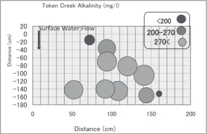
The relationships between EC and alkalinity are shown in Figure 7. Although concentrations are lower than other two spring complexes, Token Creek samples show positive linear correlation, indicating alkalinity ( HCO) is the major anion component in the Token Creek. The spatial distribution of alkalinity concentrations within Token Creek complex is shown in Figure 8. A fairly large variation was found within a meter distance, though number of samples is small. No obvious trend was found.
Figure 7 The relationship between EC and alkalinity concentrations
Figure 8 Distribution of alkalinity concentrations (mg/l) in Token Creek spring complex
4. Numerical simulation
The large spatial concentration variations observed in spring waters within a single spring complex. Numerical simulation of Token Creek watershed was performed to examine if the classical advection-dispersion equation (ADE) with reasonable degree of dispersion could produce the large chemistry variation observed.
4.1 Model design
HYDRUS2D/3D which is a finite element based software package to simulate two to three-dimensional movement of water and multiple solutes in variably-saturated media (Simunek and others, 2007) was used to examine the cause of chemistry variation found in the spring complex.
The model domain as well as generated mesh is shown in Figure 9. The model domain has a dimension of 2km in width, 5km in length and 265 to 315m in depth.
The generated FE mesh has 21100 nodes, 38019 elements and 19 layers.
The hydrostratigraphic layers (Table 1) were assigned as a simplified manner based on those employed by Dumber (2000). Six different units are assigned. From the bottom, 11 layers are assigned to represent Mt. Simon aquifer (material 3) and 12th layer was assigned to have low permeability to represent Eau Clare formation (material 4), 13th and 15th layers were assigned to have high permeability layers
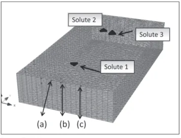
Figure 9 Model geometry (2km×5km×265‑315m) and finite element mesh (21100 nodes, 38019 elements and 19 layers) used for all calculation in this study. (a) West, (b) Centre and (c) East are observation points. Triangles on the surface are the locations of solute release.
(material 2)(Swanson et. al., 2006), while the rest of layers to the top are assigned to represent upper sandsone aquifer and unlithified layers (material 1). The elevation of top layer of the model was set to approximate topography of Token Creek watershed. The high permeability (K) layers are replaced by upper bedrock aquifer in no high K layer case in order to assess effects of high K layers. The cross section of the two high K layer (control) case is shown in Figure 10.
The boundary conditions for the flow are atmospheric and seepage at the top, no flow along all sides and bottom. The boundary conditions for transport are 3rd type at the top and no flux along all sides and bottom (Figure 11). Since an actual daily recharge rates are not known, the recharge rates are assumed to be a half of 1971‑
2000 NCDC normal monthly precipitations at Madison WSO airport (Station number 474961, Wisconsin State Climatology Office). The recharge rates are assigned uni- formly over the model and are shown in Figure 12. The same monthly variation was repeated every year for entire simulation period of 40 years. The HYDRUS calculates actual recharge rates depending on water content and hydraulic conductivity of the surface layer, so that actual recharge rates in the model may be reduced and may not be the same as the rates shown in Figure 12.
Hypothetical contaminant sources are placed on the surface at three different Figure 10 A cross section of material distribution and material properties of two high K layer case. Material 2 was replaced by material 1 in no high K layer case.
From top, material 1, material 2, material 1, material 2, material 4 and material 3 are assigned.
Porosities of all materials are 0.2, Material 1 has K=20m/day, residual water content=0,057, van Genuchten parameters alpha=12.4, n=2.28. Material 2 has K=125m/day. Material 3 has K=3 m/day. Material 4 has K=0.25m/day.
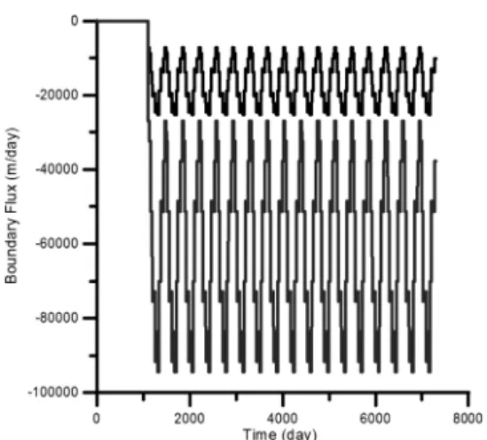
locations (Figure 9). The locations of the sources were chosen to avoid boundary effects but to test the effects of mixing of two solutes of which source areas are fairly close to each other, and also to test effects of travel distance. The solutes are placed after three years at which flow in the model is almost steady-state. The released locations of the solutes are shown in Figure 9. The solutes leach with infiltrating precipitation, and actual solute infiltration rates calculated for the first 20 years for the solutes 2 and 3 are shown in Figure 13. As initial conditions for the flow, water table was set to at 270m above sea level based on reported groundwater table in the area (Dumber, 2000). The initial condition for the transport problem was zero concentration everywhere for the three solutes.
Figure 11 Boundary conditions (a) flow: top is atmospheric and seepage face boundary, sides and bottom are no flow boundary (b) transport : top is 3 rd type boundary, sides and bottom are no flux boundary
Figure 12 Recharge rate assigned in the model
0.0016 0.0018 0.002
0.001 0.0012 0.0014
0.0004 0.0006 0.0008
Recharge rate (mm/day)
0 0.0002
J F M A M J J A S O N D
Month
(a) (b)
4.2 Concentration distribution within a single complex
The breakthrough curves observed at three different locations around the seepage face that represents spring complex are shown in Figure 14 (a), (b) and (c). Solutes 2 and 3 were placed approximately 200m apart on slightly west side from the center line of the watershed (Figure 9). Both solute 2 and 3 reached the west observation point in the spring (Figure 14 (a)) approximately 31 years after the initial release under the conditions of this study. The breakthrough curve of only solute 3 can be seen at the center observation point (Figure 14 (b)). Numerical outputs indicate that solute 2 reached at the center observation point in very low concentration. No solute breakthrough was observed at the east observation point (Figure 14 (c)). Since actual dispersivity in the area is not known, the dispersivity values of 5m were assigned all solutes. Though source areas of solute 2 and solute 3 are close by, the Figure 13 Actual solute 2 (upper) and 3 (lower) infiltration fluxes for the first 20 years.
(Inflow to the system is negative direction)
Figure 14 Breakthrough curves observed at three observation points (a) West (b) Center (c) East
(a) (b) ( c )
solutes reached the seepage face without significant mixing after 31 years. This suggests that the classical advection-dispersion equation with reasonable dispersivities could describe large chemistry variation observed in the fields. However, variation in breakthrough curves in the model exhibited spatial trends which were not found in the three field sites.
4.3 Travel distance effect
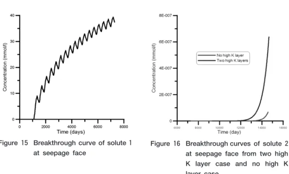
Solute 1 was placed 1.3km north of the seepage face, while solutes 2 and 3 were placed 3.9km north of the spring complex. Although no apparent seasonal variation in breakthrough curves of solutes 2 and 3 is observed (Figure 14), the breakthrough curve of solute 1 shows seasonal fluctuation (Figure 15). Temporal chemistry variations in spring waters were reported in young spring waters (Swanson et.al. 2001). The model results confirm that the spring water with seasonal fluctuation was recharged from areas relatively close to the springs and had shorter travel distance and time.
4.4 High permeability layer effect
The discharge of solute 2 at the seepage face from two high K layer (control) case and that of no high K layer case are shown in Figure 16. The solute 2 started to breakthrough approximately 31 years after the release in two high K layer case, whereas it started to breakthrough after 33 years in no high K layer case. An early breakthrough with slightly steeper breakthrough curve was found when high K layers are accounted.
Figure 15 Breakthrough curve of solute 1 at seepage face
Figure 16 Breakthrough curves of solute 2 at seepage face from two high K layer case and no high K layer case
5. Conclusions
Fast flowing springs were sampled at discharging points and analyzed for pH, EC, DO, NO‑N, Cland alkalinity within three spring complexes located near Madison Wisconsin. Chemical analysis of the spring waters indicated significant effects of land use such as road salts in urban watershed and N-fertilizer application in agricultural watershed. The chemistry distribution maps show large variations in EC and major anion concentrations even within meter-scale separation in a single complex. Despite of large spatial variation observed, no clear spatial trend was found.
Numerical simulation was conducted to examine if the large chemistry variation in spring waters observed in fields can be described by the classical advection- dispersion equation (ADE). An agricultural watershed (Token creek) was simulated using Hydrus2D/3D (Simunek and others, 2007). The different solute breakthrough curves within a single seepage face were obtained from the model based on the ADE model with reasonable dispersivity (5m). The results suggest that the solutes from different source areas in the watershed flow with little mixing and discharge into close but different points in the same spring complex. However, spatial trend was found in the breakthrough curves obtained by the simulation. Lack of gradual chemistry change observed in fields, thus, implies a presence of discrete flow paths even if it is only a short portion of the entire flow path between the source and the springs.
Conant (2004) delineated groundwater discharge zone by measuring streambed temperature distribution. Based on the observations, the groundwater-stream interactions were classified into five forms in which three discharge forms were identified ; short-circuit discharge, high discharge, and low to moderate discharge.
High flow springs sampled in this study could be one of either the first two forms of discharge. The combination of the transports by ADE with small mixing and short-circuits in the vicinity of discharging zone would result in observed chemistry variation in a small spring complex.
Numerical simulation indicated that the BTC of solute which traveled shorter distance showed seasonal fluctuation, suggesting temporal concentration change indicate short travel distance and time. Early breakthrough and a steeper breakthrough curve was found when high K layers are accounted. However qualitative effects of high K layers can not be evaluated by our model, since the porosity and recharge rates assigned in the model may be too large for the field conditions. Actual values of these are not known. Acquisition of more detailed information on distributions of porosities, recharge rates and permeability in the fields is required to better simulate and understand the flow paths and transport processes of the spring waters.
References
Bahr J and L. Parent (2001) : An improved hydrologic model for the Token creek watershed ; final report to the Wisconsin Department of Natural Resources.
Bradbury, K., S. Swanson, J. Krohelski and A. Fritz (1999) : Hydrogeology of Dane County Wisconsin. Wisconsin Geological and Natural History Survey, Open File Report 1999‑04, University of Wisconsin-Extension.
Clayton, L and J. W. Attig (1997) : Pleistocene geology of Dane County, Wisconsin.
Wisconsin Geological and Natural History Survey Bulletin 95, 64pp.
Conant Jr. B. (2004) : Delineating and quantifying ground water discharge zones using streambed temperatures. Ground Water, 42, 2, 243‑257.
Dane County Regional Planning Commission (1999) : Dane County Groundwater Protection Plan. Appendix G of the Dane county water quality plan 161p.
Hunt R. J., J. J. Steuer, M. T. C. Mansor and T. D. Bullen (2001) : Delineating a recharge area for a spring using numerical modeling, Monte Carlo Techniques, and geochemical investigation. Ground Water 39, 5, 702‑712.
Institute for Environmental Studies University of Wisconsin-Madison (1996) : Nine Springs Watershed and Environmental Corridor A Water Resources Management Study. 244p.
Lower Rock River Water Quality Management Plan, (2001)
Mazor, E. (1991) Applied chemical and isotopic groundwater hydrology, Halsted Press, a division of John Wiley & Sons, pp274.
Schafran, G. C. and C. T. Driscoll, (1993) : Flow path-composition relationships for groundwater entering an acidic lake, Water Resour. Research, 29, 1, 145‑154.
Simunek, J., M. Th. van Genuchten and M.Sejna (2007) : The HYDRUS software package for simulating the two- and three-dimensional movement of water, heat and multiple solutes in variably ‑saturated media.
Stumm, W and J. J. Morgan (1996) : Aquatic chemistry, third edition. John Wiley and sons, Inc. 1022pp.
Swanson, S. K. and J. M. Bahr (2004) Analytical and numerical models to explain steady rates of springs flow., Groundwater ; 24, 5, 747‑759.
Swanson, S. K., J. M. Bahr, K. R. Bradbury, K. M. Anderson (2006) : Evidence for preferential flow through sandstone aquifers in southern Wisconsin. Sedimentary Geology, 184, 331‑342.
Swanson, S. K., J. M. Bahr, M. T. Schwar, K. W. Potter (2001) : Two-way cluster analysis of geochemical data to constrain spring source waters. Chemical Geology, 179, 73‑91.
Wisconsin Groundwater Advisory Committee (2006) : 2006 Report to the legislature on Groundwater Management Areas. 2006 Groundwater Advisory Committee Report to the Legislature.
URL:
http://www.ncdc.noaa.gov/oa/climate/online/ccd/nrmpap.txt (January, 2009)
― Abstract ―
Spring waters were sampled within three spring complexes located near Madison Wisconsin. The water samples were analyzed for pH, EC, DO, NO‑N, CL and alkalinity A high average Clconcentration (88mg/l) with a wide range of variation (45‑135mg/l) was found in springs from an urban watershed, while high NO‑N concentration (12mg/l) with a fairly wide range (4‑20mg/l) was found in springs from one of the agricultural watersheds. Effects of land use such as road salts in urban area and N-fertilizer applications in agricultural fields are significant. The chemistry distribution maps also show large variations in EC and major anion concentrations in each single complex. Numerical simulation was conducted to understand the large chemistry variation in spring waters observed in fields. It was suggested that the combination of the transports by ADE with small mixing and short-circuits in the vicinity of discharging zone would result in observed chemistry variation.