General Statistical Treatment of Response of Nonlinear Rectifying Device to Stationary Random Input

General Statistical Treatment of Response of Nonlinear Rectifying Device to Stationary Random Input

journal or

publication title

福井大学工学部研究報告

volume 16

number 2

page range 135‑150

year 1968‑09

URL http://hdl.handle.net/10098/4870

General Statistical Treatment of Response of Nonlinear Rectifying Device to Stationary Random Input

Mitsuo OHTA* and Takuya KOIZUMI**

(Received Apr. 15, 1968)

When many correlative random physical proccesses are passed through non- linear circuit elements such as detectors or rectifiers and the output random fluctuations are considered, the probability variables defined over positive region are fundamental quantities of engineering interest.

First, a general expression of multi-dimensional probability density function in the form of orthogonal series such as statistical Hermite expansion is intro- duced. This probability expression is more general than the well-known expan- sion expression due to Gram Charlier, because it includes the latter. Then, as the special case of interest when many correlative physical quantities flu- ctuating only in positive region are treated, an explicit representation of joint probability density function in the form of statistical Laguerre expansion series is also -presented. Further, it has been pointed out that the latter method using a statistical Laguerre expansion is closely related with the statistical Hermite expansion method under a quadratic nonlinear transformation. We must call our attention to the fact that the statistical meaning

0.

e., the random property) is reflected in each expansion coefficient.

Finally, the detailed experimental considerations enough to corroborate the above theories are given for the following two cases :

(a) a quadratic rectifier with non-Gaussian random input, (b) a non-quadratic rectifier with Gaussian random input.

I Introduction

Generally speaking, there exist two modes of statistical approach toward the problem of analyzing response of nonlinear rectifying device to stationary random signal input.

In the first one it is nonlinearity itself of rectifying device that our consideration is mainly focused upon. The response of the device to random signal input is, first, analyzed in the same way as it is when the input signal is entirely deterministic, and then the probability distribution of the random signal is taken into consideration. The second way of approach is in rather striking contrast to the former. First of all, we notice a random fluctuation itself of the output caused by that of the input before we proceed to any analytical treatment of the nonlinearity. Then, the effect of the non- linearity which may appear as a difference between the input probability density and

*

Professor,

**

Assistant

the corresponding output one is reflected in the parameters of the output probability distribution. ¹⁾

The fonner, we can say, is an orthodox method and is effective when we desire to analyze the relation between the output distribution density and the nonlinearity in the form of time series. The effectiveness, however, is limited to situations where we have combinations of comparatively simple nonlinear functions and distribution densities with a single or two random variables at most. We may encounter with a great analytical difficulty when we have to deal with the multivariate probability distribution density of the output of intricate nonlinear device.

The latter might be said to be in the reversed situation vis-a-vis the former because what is demerits with the former is the latter's merits and vice versa In order to express canonically many types of the distribution densities of nonlinear device output, the nonlinearity inherent in such a device is given only the secondary importance and is taken into consideration directly in the parameters of the distribution through the moments.

A variety of nonlinear devices. such as detectors or rectifiers. are now in wide use both in physical and engineering fields. So these devices might deserve a further attention and investigation at the moment. Actual measurements are always accompanied by extraneous noise disturbances and these disturbances degrade more or less the precision of our measurements. Therefore it is impossible to neglect the effect of noise in our treatment of nonlinear device. In the present paper we have obtained a canonical form for the responses of various nonlinear rectifying devices, where we have specifically considered two cases: 1) the output fluctuation is limited to positive or negative region, 2) the output fluctuates in an arbitrary semi-infinite region. We bave made a couple of experiments on two extreme cases and the theory has been confirmed to be in close agreement with our experiments. Our method of analysis is based on the latter method mentioned above.

II Theory

2.1 General representation of probability density function for the output of nonlinear device

First. in the random fluctuation of the output of an arbitrary nonlinear system.

which represents a stochastic process, we notice some basic and common properties manifested throughout the entire random variations. e. g .• a boundary region where the fluctuation takes place. like ( - <Xl ,

+

<Xl). ( - <Xl. 0

J.

or [ 0 ,

+

^<Xl). Our next step is, then, to obtain the probability distribution density of the output expressed in the form of an orthononnal expansion, each coefficient of which may be expressed as a function of mean value, variance. high order moments etc., so that the effect of the transfer characteristic of nonlinear device upon the input is reflected in it. If we find more evident properties or informations contained in the output which reveals us more knowledge about the process at hand, we, of course, need to have the scope of our search narrowed down according to the new constraints we have found.

Now, we will let p (Xh X2, """, XK) denote the joint probability distribution density function of K random variables Xi (i

=

1. 2. . ... , K). each of which represents the output of K distinct nonlinear rectifying devices. We will expand the probability density function in the series in terms of orthonormal functions.²) Its correlation effect and statistical properties of the output will be retained in the coefficients of the expansion. Without any loss of generality the random variables Xi can be assumed to fluctuate irregularly within closed regions [ai. biJ. On the basis of the mean-square·

error criterion the joint probability density function of the output can be expressed as

.... ·· .. ·(1)

where

K

a(nh na. · .... ·,nK)= <IT<'on;(Xi))

i=l

J

^b

1J

^b

2 fbk K

== ...

:IT

<,Oni(Xi)·P(XhXa' ... XK)dXtodXa .. ·,,·dXK. · .. · .. · .. (2)

al a2 ak ~-1

and (

>

denotes statistical average over Xh X2, ... , XK. {<,Oni (Xi)} form a complete set of orthonormal functions with respect to the weighting functions d(xi)

f

^bi

(<'omi. <'on;)

==

<'omi(Xi)<'oni(Xi)d(Xi)dXi= Omwi.

ai

.. · ... (3)

Next problem for us to solve is how to let each coefficient of the expansion bear the marks of nonlinear effects. However, the fact that each coefficient can be given in terms of joint moments of the form (Xl l^! X2l2 ... XK lk

>

^(li; arbitrary positive integers) suggests us that this can be done by coloring each joint moment with the nonlinear effects in whatever manner.

If we are to be strict, there may not exist any perfect zero-memory nonlinear device, since we know that the so-called inertial effect or integration effect in nonlinear system, which is attributable to the time constant and the frequency response of the system, is nothing but a memory marked on its output of the past record of input, but we also know that without this effect the nonlinear system cannot perform effectively its nonlinear action on the output. The extent of this difficulty, however, can be dimi·

nished by redefining the function of a given nonlinear element as .. zero-memory non- linear transform" plus "linear integration effect" according to N. Wiener' ssuggestion.

In fact we can solve many practical problems involving nonlinear devices by this concept of approximation.

Now, let f ( ) and h (t) represent the "zero-memory nonlinear transform" and the impulse response function for the "linear integration effect" respectively. The output of a given nonlinear device can be given by

Xt(t) = f~h(t")f(Zl(t-t").Z2(t-t")." .... ,Zs(t-t'))dt', .... · .... (4)

where we have made an assumption that S input signals Zi(t) (i=l, 2, ... , S) yield a nonlinear output Xi (t). If necessary statistical properties of the inputs are previously given, joint moment of any order with respect to Xi (t), (X1t¹ X2t2 ... XKlk), can be calculated from the relation (4), and the result, when substituted in Eq. (1), gives us

the joint probability density which meets the aforementioned requirement that statisti- cal properties of input signals and nonlinear transfer characteristic of a given device should be reflected in the probability density for output, or more specifically, in all the coefficients of its orthonormal expansion. Obviously, it is the "zero-memory nonlinear transform" Xi = f (Zh Z2'···, ^ZK) ,that causes the most significant change in the statis- tical properties of the inputs. Nonlinear device usually comprises some components or elements. Provided that we are given the operational characteristic of each component of a given nonlinear device, the knowledge of each of the characteristics can be our foundation on which we can set up the analysis of the nonlinear device. What we are aiming at here, however, is to introduce a more universal statistical procedure which is applicable to the analysis of any nonlinear device. This procedure is based upon the extraction of some consistent properties of the irregularly ever-changing output of the device. So our consideration will be focused upon the embodiment of Eq. (1) rather than that of Eq. (4).

Since nonlinear element, whatever it is, always produces an output fluctuation in the region (-00.+00), we can set in Eq. (3) ai= -00, bi

=

+oo(i=l, 2.···, K). Hence, we may need to employ the Hermite polynmials as the orthonormal functions ({JDi (Xi) in the region. We can obtain the following relations corresponding to Eqs. (1) and (2):

A(nl.nz •...• nK)=<-n-~Hni i=l ni. ^(Xi-I!!;) \y Ai

>

• ... ·(6)

where 1 X"

<pni (Xi) _ / _{v ni.} r {I 2 A _{7r i} Hni (- ; _V

=,'!!:)

_{IIi •}

•... (7) d(Xi) = exp { - ~-:-(Xi - J.ti)Z }

2 ^{t •}

and

> )'

is a summation with respect to all ni except nl=n2= ... =nK= O.

nhnZ ... nK> 0

It is natural to impose the conditions:

ni

ni ... ·(8)

A(O.O ... O. 1 .0 ... 0)= 0 (nj=Oji.Vj) , } A(O,O ... 0.2,0 ... 0) = 0 (nj= 20ji , Vj)

on Eq. (5) so that the approximation by the first term only may become sufficient for practical purposes and furthermore the unknown parameters Pi and Ai may be deter- mined from given statistical data by means of the method of moment. Namely, from Eqs. (6) and (8), the statistical meaning of the two kinds of parameters are found as follows:

J.ti = <Xi) (mean) , Ai =«Xi - J.ti)Z)=C1xiZ(variance). · .... · .. ·(9)

Finally, we can derive a set of properties:

ni nl

A(O, ... 0, 1 ,0 ... 0. 1 .0 ... ,0) =P(Xi,Xj)(nL =Oti+OO. vI).

~ ~ 1

A(O ... ··.0.2 .. 0 ... 0.1.0. · .... ·.0.)

=

v-ZP(Xiz.Xj)(nt=20ti+Otl.Vl).

nt nj

A(O ... 0.2.0 ... · .. ·.0.2,0, ... 0) =iP(Xiz.Xi)(nL= 2 ((hi+Oli).VI) ,

\ ••••••. "(IOJ

_ H

₁ (Xf-fJj)

_dXj

+

. . . : : : ; . . . . - - - '

> ) ,,<K JII

^{_l-H nil ni (Xi -}dXi

^fJi) >

^H nJ ^{(Xl -}dXI

^fJl)

( X2 -

1l2) (XK - ilK)}

- Hng - - .. ····HnK - - -

dX2 d X K . ···(ll}

where p eXin, Xjm) en, m: positive integers) stand for the coefficients of correlation function between the n-th power of Xi and m-th power of Xj, and

> : "

excludes (nhn2) = (0,0), (0,1), (1,0), (0,2), (2,0), (1,1). In Eq. (11) we need to note that the ordinary first order correlation functions P (Xi. Xj) come first in the compensation terms and further that the correlation functions of higher orders must be taken into consideration.

Specifically, when k= 1, Eq. (11) is identical with the well-known Gram-Charlier series of type A in mathematical statistics:

P(X)

=

_1 {fDo(X-J-!)_~~-fD8(X~,u)+~-(J)4(X-,u)_ ... } ... (12)

dX dX 3. d.\ 4. dX

Here, ra and r4 are statistical quantities called skewness and kurtosis respectively, which characterize the shape of distribution density. (/)o(X) and (/)m(X) are defined as

X² 1 - 2 -

fDo(X) =y

21t

^e .

d^m

fDm(X)

=

dxmfDo(X)

= (-

1 )maJo(X)Hm(X).

I

f

..· ... (13)

The first term of Eq. (12) is obviously Gaussian probability density function. In fact Eq. (12) is frequently useful, when we want to analyze the response of wide class of nonlinear elements to random input, particularly when the input-output characteristic of an element is of odd function type (e.g., relay element at).d element with saturation).a.14) Since the output fluctuation of rectifying element necessarily occurs within e -00,+=), it is possible to use Eq. (12) as the probability density for the output. But unlike the other non-rectifying nonlinear elements every rectifying element produces an output fluctuation in which an evident common characteristic can always be : observed. The positive use of the characteristic will bring us to our end, that is, the derivation of universal method for the analysis of nonlinear rectifying element.

2-2 Probability density functions for the output of nonlinear rectifying element 2-2-1 Multivariate case

Since it gives not only a good practice but also a good approximation in our succeed- ing analysis to limit the output fluctuation of nonlinear rectifying element within a region [0,

+

=), we can set ai= 0 and bi=

+

00 in Eq. (3) without loss of generality.

We will use the Laguerre polinomials as the orthonormal functions ^<pui (Xi) in the specified region. Corresponding to Eqs. (1) and (2), we can derive respectively

where

d(Xi) =Xim;-l • exp {-Xi/Si} .

}

As in Eq. (8). we naturally impose the following conditions:

ni

B(O.O.···.O. 1 .0.···,0)= 0 (nj=Dji,Vj)

ni

B(O.O, .. " .. ,0,2.0 ... ,0)

=

⁰ (nj=2Dji, Vj)

)

•·· ... U4) ...•..• "(15)

···U6l

on Eq. (14) partly because we desire to approximate Eq. (14) with its first term and partly because we desire to have S i and mi determined statistically by the method of moment. In other words. from Eqs. (15) and (I7) the statistical estimate of

Simi=(Xi) (mean),

Si²mt(mi+ 1) = (Xi2) (second order moment).

or

mi = (Xi)2/d.Yi2 , Si =dXi²/(Xi) (dXi²=«(Xi - (Xi) )2) =Si².mt) will be obtained.

}

.. •·•·· .. U8)

.... • .... (19)

Thus we can derive the following expressions in like manner as in the previous section (cf. Eqs. (10) and (11)) :

ni nj

B(O, ... ,0, 1 .0, ... ,0, 1 ,0, ... ,0) _{y minj} P(Xi.Xj)(nl=Dli+Olj.Vl).

1

ni nj _ _

B(O, ... ~O. 2 ,0, ... ,0, 1 ,0, ... ,0) =P(Xt.Xj)"/ mimj (mi+ 1)

J'

--2-P(Xi2, Xj)ymimj(mi+ 1) (4mi+ 6) (nl=2oli+olj.VI),

... (20)

... (21)

In each coefficient of the expansion is a statistical reflect of correlations of all orders and high order moments. Here, the Laguerre polynomials are defined as

ex.X-

a (~)n{e-x.xn+a} =:fi(n+':) (-~)i.

n! dX j=O n - J J! .. ... (22)

The high order moments based on the expanded form of the joint probability density function Eq. (21") are, with the help of

f

^{OOxl+m-l. e-X •} L<m-1l(X)dX r(l+m) rCn-1)

o n n!r( -I) ••• ... (23)

given as

<x

I1X 12

X

^{IK) -}

Tr

Si'iT(mi+li) •

{1 ^{+ ~P(Xi,Xj)}

^{( -li)( -Ij)}

1 2 ... K _i=l T(mi) i>jY mimj

••••••••• (24)

where

(-I)n=( -/)( -1+ 1)( -1+ 2) .. · .. ·( -I+n- 1).

2-2-2 A single variable case

If we set k= 1 in Eqs. (19) and (21), then at once the Laguerre expansion of the probability density function of nonlinear rectifier output in case of single variable is obtained as

PCX)

=

1 xm-l • e-x/s {I +

IJ

^{n!rCm) (L (m-I) CXIS)}

>

^{L (m-I) CXIS)}.} . ... (25)

rCm) Sm n=arCn+m) n n

and its parameters also are calculated from

m = <X>2/^qx2 , S=(X>lm. · ... (26)

The high order moments are derived from Eq. (24) as

(Xl) = SLrCm+/) {I

+IJ

nlrCm) (L(m-l) (XIS) C-I?n}

rCm) n=sr(n+m) n n . . • .... · .. ·(27)

Obviously, the first term of Eq. (25) is the Gamma distribution density function, and the second and the higher terms give the estimate of deviation from tl,tis particular probability density function. In Eq. (27)

~

can be approximated with a finite number

n-3

of terms when I is a positive integer.

The quantities of skewness and kurtosis are used to give a quantitative estimate of the deviation of the probability density function Eq. (11) with k= 1 or Eq. (12) from the Gaussian distribution density function that is the first term of each expansion expression. From this point of view we may introduce new quantitative expression for each of the skewness and kurtosis on the basis of the Gamma probability density function, namely, the first term of Eq. (25). If we denote each expansion coefficient inside the brace in Eq. (25) with Bn, the third and the fourth order moments about the mean can be expressed, from Eq. (27), as

ox⁸==«X-(X»)8)=(X3)- 3 (X²)(X) + 2 (X)8= 2 ms8 - mCm+ 1 )Cm+ 2 )Bs^·S8, .... ·· .. ·(28) rx4==«(X-(X»)4) = 3 mCm+ 2 )S4-B4·m(m+ ¹ )Cm+ 2 )Cm+ 3 )S4. ..· ... (29) If we note here ~hat Ba and B4 in Eq. (25) correspond to

r3

and

r4

in Eq. (12) and that the first terms of Eqs. (28) and (29) respectively give

ox

³ and

rxt

of the Gamma distribution density function itself when Ba = B4

=

0, we can introduce our new and reasonable definition of skewness and kurtosis as

(

OXS _ _ 2 .) __ _ (m+ 1). Cm+ 2)B.

skewness : ~

qx^B

vm vm .

• ... (30)

kurtosis (rx4 _ 3 m+ 2)= _ Cm+ 1) (m+ 2) Cm+ 3)B

4 ,

qx⁴ m m ... (3~

where

B

==

n!rCm) (L (m-I) CXIS) nlrCm) ~ (n+~ ^{- 1) (} ~ 1 )i (Xi> ... (32)

n rCm+n) n r(m+n)i=O n-J JISi •

One thing to draw our attention here is that in the calculation of Eqs. (29) and (31) we

set Ba= 0 as in Eq. (12) in order to let the expansion coefficient B4 have a reflect of kurtosis regardless of Ba.

2-3 Relation of the statistical Hermite expansion with the statistical Laguerre expansion

We have already learned the fact that the statistical Hermite expansion is applicable to the problem of random fluctuation distribution within the region (-00,

+

00) while the statistical Laguerre expansion can be applied to the distribution of fluctuation in the region [0,+00). This fact naturally leads to an idea that for the representation of distribution density of random input for a nonlinear rectifying element Eq. (11) is suitable and to random output fluctuation Eq. (21) is applicable.

Let us now consider the case of a single input. We assume that we have here as a nonlinear rectifying device corresponding to Eq. (4) a mean-squaring circuit ^5,6) which can be expressed analytically as

J

^{oo 1}

JT

X(t)= h(r)ef(Z(t-T))dr =~ Z2(t-.)dr.

o T ⁰ ., •..••. '(33)

and further that white noise input z (t) is applied to it. Using the Fourier series representation of white noise of bandwidth Wand duration T (averaging time) due to S. O. Rice,7) we can readily obtain

1 N K

X ^=----Lj {ai+bi}

=

^LjXi2 (aj, bj : Fourier expansion coefficient),

2 j=1 i=l

••••••••• (34)

where

Xi =aj / y2 or bj / y2 . .. ... ·(35)

If the noise characteristics are taken into consideration. Xi are mutually independent random variables and are normally distributed with the mean Pi and variance ^{aXi2 :}

J1.i=(Xi>= 0 • qXi2=«Xi - J1.i)2>=qo2 (a constant). .. ... ·(36)

Their moments are given by

... (37) It is obvious that the joint probability density p (XIt X2 .. ···.XK) for K input variables is given by the first term of Eq. (11) that is the product of K mutually independent one-dimensional Gaussian density functions.

Therefore, in this case

<

^{Hni ( :;}

»=

^{0 (ni> 1) .} ..· .. · .. ·(38)

On the other hand, the output probability density p (x) is given by Eq. (25). Using the following properties obtained from Eqs. (34), (36) and (37),

<x> =K^eQ02. <X²>

=

I.i<Xi4)+ I.:L:<Xi2><xi> = 2 KQ04+K2Qo\ Qx2 = 2 Kq04. .. ... (39)

i i~j

the parameters m and s are determined as

m=K/2. S=2q 02. • ... (40)

SpeciallY, it should be noted here that the number of dimensions K becomes 2TW which is a number defined as the freedom of sampling space by C. E. Shannon^S) when T is large. With the help of Eqs. (34), (38) and (40)

<

L\m-I) (x/s)= <L

(~-1) (-l-z-f Xi2)

n n 2 dO i"'i

K 1

= ? : 1f <L ^-.'1 (Xi2/2doZ) Pl+P2+ ... +Pg=n. 1"'1 p~

=

> : IT

^1. <H2.o;(Xi/do) = 0 ... ' .. (41)

Pl+P~+""'+PK=n. ^{i=1 ( -} 2) P^t Pi!

is obtained, hence the probability density for the nonlinear output of Eq. (33) can be exactly represented with the first term of Eq. (25) that is the Gamma probability density function. We have made the above analysis to show a mutual relation between Eq. (11) and Eq. (25), but it would be more convenient to utilize the regenerative property of the Chi-square distribution, if we wanted just to derive the distribution of the output of the mean-squaring circuit.

Thus, we can say in conclusion that the terms higher than the second in Eq. (25)

0.

e., the deviation from the Gamma distribution) become significant :

i) when the probability distribution of the input is non-Gaussian and the rectification is full-wave quadratic,

ii) when other types of rectifier are used with an input having Gaussian probability distribution.

In particular case where an additive combination of stationary random signal and deterministic signal exists in the input, the deviation from the Gamma distribution becomes important.^9,10)

III. Experiment

3-1 Confinuation by experiment

By means of experiment we have confirmed the validity of Eqs. (21) and (25) when applied to some practical problems. Any record of random output of rectifier with an ideal rectification characteristic can be an object of the confirmation by experiment if the probability density of the output has higher terms which cannot be neglected vis- a-vis the first term, since the expressions of Eqs. (21) and (25) are applicable to output of any type of nonlinear rectifier with stationary random input when the output fluctuates only in the positive region and it has a definite probability distribution.

3-1-1 Method of confirmation of distribution parameters and high order moments First, a photograph of waveform from a rectifier is taken and enlarged. and then the waveform is sampled with an equal time interval. The vertical axis is divided up into a number of sections spaced with an equal interval. If we count directly or by the use of counter a number

Ii

of sample points on the waveform which appear within Xi-th section (corresponding to Xi-th level), then the n-th order moment

<xn)

can be given by

~£;:\

where, of course, the Sheppard's correction has to be made when the dis- tribution curve has a contact of high order with the horizontal axis.

From (X) and (X2) thus obtained the parameters m and s are calculated by the use of Eq. (26). These parameters when substituted in Eq. (27) gives a theoretical value of

I-th order moment ^<xt) (1) 3), and comparing this ^(xt) with the other one obtained experimentally, we can confirm that the relaton (27) holds in this particular case.

Obviously it does not make any sense to try to confirm Eq. (27) by the above experi- mental procedure when 1=1 or 2. For simplicity and convenience some specific forms of Eq. (27) are written below :

<X⁸)=m(m+ 1 )(m+ 2)sa{ 1 -B8) . }

(X4)=m(m+ 1 )(m+ 2)(m+ 3)S4{ 1 - 4 Ba+B4} ,

(X5)=m(m+ 1 )(m+ 2)(m+ 3)(m+ 4 )S5{ 1 -lOB_a

+

5B4-B5}.

... (42)

In a similar fashion the statistical quantities given by Eqs. (30) and (31) can also be confirmed experimentally.

3-1-2 Method of confirmation of distribution curve We know the following facts concerning Eq. (25) :

i) truncation of Eq. (25) with a finite number of terms by discarding higher order terms will have no effect upon the condition

J ^~

P(X)dX= 1 ,

ii) in engineering practice cumulative probability distribution is frequently of more importance than probability density.

So, we observe, in theoretical cumulative probability distributions for

Pl(X) r(~) smxm-l

• e -x/S(r-distribution). .. .... • .. (43)

Pa(X) r(:) smXm-¹ e, e -XIS. {I +BaeLjm-l\x/s)}, ... (44)

Pa(X)

r(m\

^{smXm-1 e e -XIS. {I} +Ba.L~m-l)(x/s)+B4. L~m-l)(x/S)} , • .. • .. • .. (45)

an effect of successive addition of higher term upon the betterment of approximation of each distribution for the cumulative frequency distribution which has been obtained experimentally. To be concrete, we first draw curves of the experimental frequency

Transformation Phase

Integrat ing ^between

White Gaussian inverter

noise !---::o circuit ~ non-Gaussian ^and f---.:> type

~enerator I ^type squaring

random

fluctuations circuit

1

₁

_L

Constant

Integrating voltage

circuit power

supply II

B

rathode-ra

White

Band-pass pscilloscope

noise ~ f---.I. ~ with

generator fi Iter single

sweep

1

Constant

l

^{voltage power}

(a) Experiment A. lCathode-ra, supply

oscilloscope with

single (b) Experiment B.

sweep

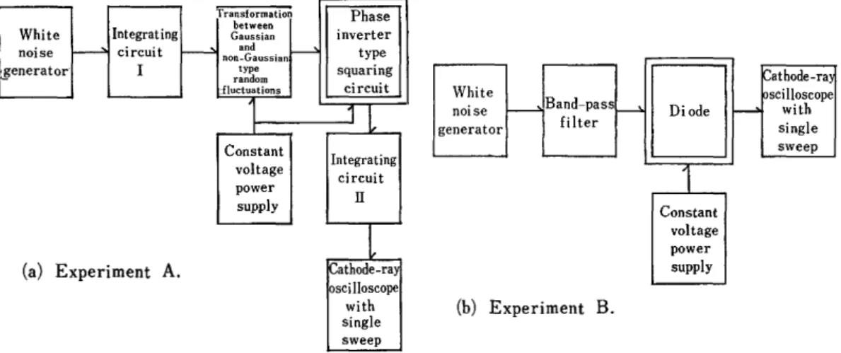
Fig. 1 Block diagram of experimental system for measuring the response of nonlinear rectifying elements to (a) non-Gaussian and (b) Gaussian random inputs.

distribution and the theoretical distribution densities given by Eqs. (43) to (45) in which the values of m. s. and Bn of Eq. (32) are substituted. and then comparison is made of each of the cumulative distribution curves obtained from the above density curves by the use of planimeter.

*

The procedure is similar to that of applying a distribution to the Gram~Charlier series.

3-2 Systems of experiment

As we mentioned in Section 2. 3. we have made a couple of experiments on two expreme cases as follows :

A ') (Non~Gaussian input)

+

(quadratic rectifier).

B) (Gaussian input)

+

(non~quadratic rectifier).

The block diagram of measuring system for each of the above cases A) and B) is shown in Fig.l (a) and Fig. 1 (b) respectively. As the squarer in Fig. 1 (a) a phase~inverter type squaring circuit which shows an excellent quadratic characteristic even with as high input level as 500 mV is used. and as the non~quadratic rectifier a diode is employed.

The input~output characteristic of the former is depicted in Fig. 2. Integrating circuits and a bandpass filter are used to facilitate counting the frequencies of output waveforms by eliminating high frequency portion of energy out of the input.

**

^If we use the fact that non~Gaussian distributions lack in symmetry. we can check if a given random input wave is normally distributed. To be specific. we have used the fact that a non~

Gaussian random noise produces on cathode~ray oscilloscope a vertical line with asym~

metrical brightness distribution when the horizontal gain is reduced to zero. The noise generator we have used produces a white noise with uniform spectrum between lOc/s and IOkc. Time constants of the integrating circuits I and II are chosen to be 2KtJ x

o

.1.uF and 500KtJ x O. OOI.uF respectively.

Use is made of the mutual characteristic of triode near saturation region to trans~

form the noise wave from the noise ge~

nerator into a typical wave of non~Ga~

ussian type.

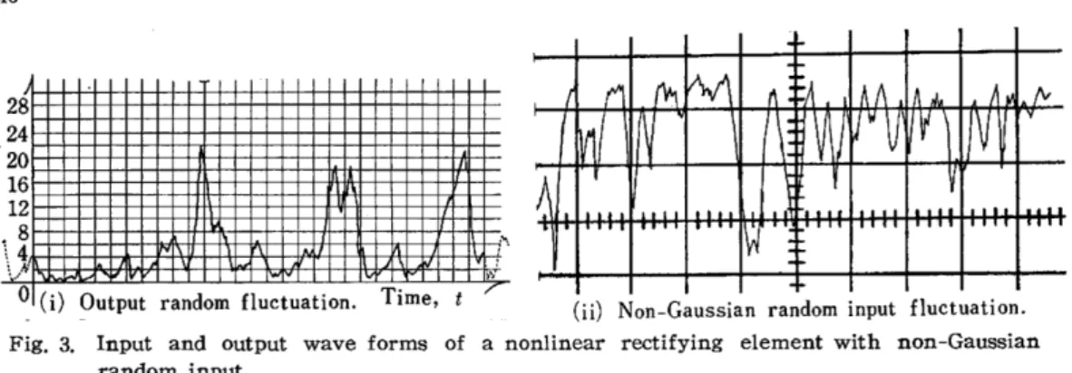
3-3 Results of the experimnt 3-3-1 Input and output wavefonns Fig. 3 (i) and (ii) show typical wa~

veforms we have observed in the ^ex~

periment A respectively of the input and output of the nonlinear rectifier.

3-3-2 Frequency distributions In Fig. 4 (a). (b) are plotted the

I

"

50 ....

f ^{

3,0 ^~.

I

J

^,

-

II

- ¹⁰ - ⁹ ₈

- _{7- l'}

6 I

5

.t /

I I

2

V-J:!a~~l?

- ^{1 -}

2-

^{3- -5 678 1 0 -~O-3}

Input voltage (XI0²mV) Fig. 2. Characteristic curve of a phase

inverter type squaring circuit.

*

As in the check of the Gram-Charlier type A curve, check can be made for the fitness of distribution by the Chi-square test.

** The addition of these linear elements does not change the fundamental property of rectifier that the output fluctuations occur only in positive region.

28 24 20 16 12

. 8 ^{I ~} _:~

\ 4 ^IN

\ ....

'"

^{I'" IV ~V}

0 i Ou ( ) tp t u random fl uc t ua t' on. Time, t ^{/ '} (ij) Non-Gaussian random input fluctuation.

Fig. 3. Input and output wave forms of a nonlinear rectifying element with non-Gaussian random input.

frequency distributions based on the observation of waveforms in the experiments A and B. The existence of a couple of humps in (a) can be easily understood if we think of how the non' Gaussian input wave is produced.

I I

/ vI\ ^{J I I} I I I I I I I I I I

10 0 / \ I I I I I I I I I

I (a) Experiment A.

0 ^{1\ i}

J \

0 II i

i\

10 Or--

N

I I I I I I I I IJ-_f-'-

I ...,

(b) Experiment B .

0 ^{f - -}

"-

I \

0

'"

^{"- I}

8

o

^{2 4 6} 8 10 12 14 16 18 20 22 0 0 2 4 6 8 10 12 14 16 18 20

Level Xi Level, Xi

o I

f r---.r-... .... ---

""

Oll ^1'\

. r -

II ""-..,

... ...,

~

2

0 f'"

01-^.. _- ""'r-..,.

-""r---.r--., ... --

/ '

Fig. 4. Experimental results indicating the frequency distribution function for the response of nonlinear elements to (a) non-Gaussian and (b) Gaussian random inputs.

3-3-3 Hvaluation of the parameters and moments

Care has been taken in drawing the frequency distribution curves to make them as smooth as possible in expectation of errors in counting the frequency of each level and of the continuity of distributions.* We will later compare those curves with the the- oretical distribution curves.

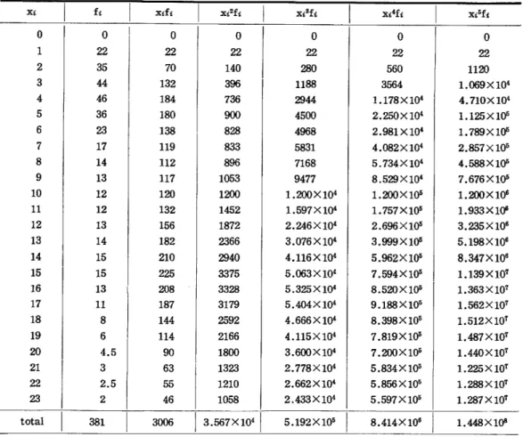
Table 1 has been prepared to evaluate various moments up to the order of five on the basis of the frequency distribution curve for the experiment A. A similar table for the experiment B has been omitted because of limited space.

[Experiment AJ

Experimental values for the moments are

<X)=7.808, <X2)= 92. 64(O'x² = 31.68) • <X8)

=

1349,

<X4) =2.185X 10\ <X5) =3.761 X 10⁵•

Thus from Eq. (26) m=1.925. S=4.056.

* Since the experiment governs the individual data while the theory governs a relation existing among the data, it will be reasonable in drawing experimental curves to connect each of mea- sured points with a smooth curve so that entirely smooth curves may come out if these curves have to be compared with theoretical ones at all.

Table 1. Calculation of five moments in the experiment A.

Xi

0 0 ^I 0 0 0 0

1 22 22 22 22 22

2 35 70 140 280 560

3 44 132 396 1188 3564

4 46 184 736 2944 1. 178X10'

5 36 180 900 4500 2.250X 10'

6 23 138 828 4968 2.981X10'

7 17 119 833 5831 4.082X104

8 14 112 896 7168 5.734X104

9 13 117 1053 9477 8.529X10'

10 12 120 1200 1. 200 X 10⁴ 1.200X1Q5

11 12 132 1452 1.597XIO' 1. 757 X 10°

12 13 156 1872 2.246XlO' 2.696XIQ5

13 14 182 2366 3.076X104 3.999XIQ5

14 15 210 2940 4.116XI04 5.962X10⁵

I

15 15 225 3375 5.063XI04 7.594X10°

16 13 208 3328 5.325XIO' 8.52OXIQ5

17 11 187 3179 5.404X104 9.188XI05

18 8 144 2592 4.666XI04 8.398XI05

19 6 114 2166 4.115X 104 7.819X1Q5

20 4.5 90 1800 3.600XI0⁴ 7.200X105

21 3 63 1323 2.778XI04 5.834XI0⁵

22 2.5 55 1210 2.662X104 5.856 X 105

23 2 46 1058 2.433X104 5.597X105

total 381 3006

I

3.567XI041 5.192X10⁵

I

^8.414X106

I

[Experiment BJ In like manner

<'X)=5.868. <X2) =57 .13(l1x²=22. 7),

<X8) =683. (X⁴)=9.06X10³,

m

=

1. 52, S = 3. 87 •

}

3-4 Comparison of experimental values with theoretical ones 3-4-1 High order moments

From Eq. (32) the Laguerre expansion coefficients are found to be B3=0.0856. B4=0.0845 (experiment A),

B3=0.12O. B,=-0.174 (experiment B).

0 22 1120 1. 069 X 10⁴ 4. 710X 10⁴ 1.125X105 1.789X1Q5 2.857X 105 4.588 X 1Q5 7.676 X 10⁵ 1. 200 X 10⁶ 1.933 X 10' 3.235XI0⁶ 5.198XI0⁶ 8.347XI0⁶ 1.139XI0'T 1.363XI0'T 1.562X10'T 1.512XIO'T 1.487XI0'T 1.440XI0'T 1.225XI0'T 1.288 X 10'T 1.287X10'T 1. 448 X lOS

As is clear from Table 1, the higher the order of moment is, the larger value of X the weight is laid upon. The deviation naturally tends to become large as the order of moment increases, since the frequency of the output waveform's passing through sections of higher levels is much less than that of its passing through lower sections and as a consequence an error in counting the frequencies for those higher levels inevitably increases. In many practical problems in engineering, however, to secure a precision in the measurement of low order moments is important.

3-4-2 Skewness and kurtosis

Upon the experimental determination of the left-hand sides of Eqs. (30), (31) toge- ther with the values of m these will be compared with the right-hand sides. A quite good agreement between the experimental values and theoretical ones can be seen.

[Experiment AJ

skewness : - 0.7080 (theoretical value - 0.7083) , kurtosis -5.210 (theoretical value - 2.482).

[Experiment

BJ

skewness : -0.898 (theoretical value -0.870).

Since Ba is a little too large to be regarded as zero, the kurtosis is not available for this case as is clear from the discussion given in Section 2.2.2. In general, experimental values of kurtosis are worse than those of skewness in their agreement with theoretical values. This fact can be explained with the same inference as the one for the moments in Sec. 3.4.1.

/

10 0

~ 8

:3

_;;;S

~7 1: _(fJ 0 0 0 .:a 6 0 0

I--

01---

I---

01-- I-- 0

AI

II!

+--~

I - /.~

1-~1 'il

QF _Ii

WI

"

0

E

[If'

- ^,

^{I r}

",'ii'" ,J~ ^1----

~

Vr

,:i

^v

"f' ^'/

/.1/

,1/

iT (a) _-

Experiment A. -l-

c ^Q 0 - -+-

Experimenta I curve ----,--- -+-

10 P, (x)dx Theoretic

~7r:J~~x

10' P. (x)dx curve

--t- - l -

---

o

0 2 4 6 8 10 12 14 16 18 20 22 Level, Xi "

-

I f /

10 0

"T);~ ^{~ ;--}

0 7)'',('

~

,:~

/;~

-

^/

0

I '~f.1 0 ^-:~ 'fI

,if

~~

^{t--f - (b) -}

0 - Experiment B. -

I--+-- - o Q Q -

01--+--/r, Experimental curve

FJ' ---j -

f - lo' p, (x)dx

0 j-;;,(;td-; Theoretica

,;:'

^-"1₀^'

j,:r;,'d-:

^c:v;s

11//

0 :

at

°7i/f k

'I-- I--+-

o

^II:

II,'

002 4 6 8 10 12 14 16 18 20 22

.

Level, Xi

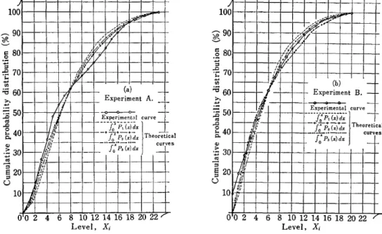
Fig. 5. Experimental and theoretical probability distribution for the response of nonlinear elements to (a) non-Gaussian and (b) Gaussian random inputs.

3-4-3 Cumulative probability distributions

First, upon the substitution of the values of m, s, and Bn in Eqs. (43) to (45), the numerical calculation of values of PI (X), plX) and Pa(X) for each level of X is made, then these are plotted on a section paper together with the earlier experimental fre- quency distribution, and finally, a cumulative distribution curve is drawn for each of the above theoretical and experimental distribution density curves by means of planimeter.

The result is shown in Fig. (5).

Fig. 5 (a) pertains to the experiment A. The effect of higher terms in the Laguerre expansion can be clearly seen therein, i. e., the addition of a higher term to the funda·

mental Gamma probability density function PI (X), which actually yields P2 (X), has brought the latter closer in position to the experimental distribution curve than the former. and likewise Pa(X) which has one more higher term than P2(X) is closer to the experimental curve than P2 (X) is.

Fig. 5 (b) shows the result for the experiment B. Unlike the above situation the successive addition of higher terms of the Laguerre expansion results in the oscillatory converging of theoretical curves to the experimental one. So it is difficult to say whether J:P3(X)dX or J:P2(X)dX is closer to experimental value than the other. It is. however. evident that the addition of any higher term gives at least a better appro- ximation.

IV. Conclusion

What we have done in this paper is summarized as follows.

1. The principle of statistical treatment for the multivariate joint probability dist~

ribution of the output of nonlinear element with stationary random input as well as the general explicit representation of the Hermite expansion of the multivariate joint probability distribution which reduces to the Gram~Char1ier series when with a single variable have been given.

2. The Laguerre expansion for the multivariate joint probability distribution of the output of an arbitrary nonlinear rectifying element, fluctuation of which takes place in [ 0,+ 00), has been given. and how the nonlinear effect and the statistical reflect of correlation and high order moments are retained in expansion coefficients has been shown.

3. The relation between the Hermite expansion for probability distribution of input wave for a quadratic nonlinear device and the Laguerre expansion for probability distribution of output wave has been investigated.

4. Observing the fact that the first two terms of the Gram~Charlier series are related to skewness and kurtosis defined on the basis of the first term that is the Gaussian distribution. a new definition of those on the basis of the Gamma distribution that is the first term of the Laguerre expansion has been introduced.

5. The theoretical relation of such statistical quantities as high order moments.

skewness and kurtosis for probability distribution of the output of the nonlinear recti- fying element with the Laguerre expansion type representation of probability distri- bution has been derived. and furthermore the existence of this relation has been con- firmed by means of two model experiments:

A) (Gaussian input)

+

(non-quadratic rectifier), B) (non-Gaussian input)

+

(quadratic rectifier).

6. How in the Laguerre expansion type representation of probability distribution the successive addition of higher terms moves theoretical cumulative probability distri- bution curves closer to experimental cumulative frequency distribution curve has been observed from the above model experiments.

Acknowledgments

The authors wish to thank Prof. Isao Takahashi of Kyoto University for his helpful instruction and invaluable criticism. The authors also wish to record their appreciation of the great assistace of Mr. Isao Fukuchi, Mr. Kiyomichi Atobe and Mr. Yutaka Ta- naka in dealing with an amount of data.

A part of the present paper has been published in the July (1968) issue of IEEE Transactions on Information Theoryll>.

References

1) M. Ohta : Report to Symposium at Kansai Meeting of Electrical Society of Japan (1957) 307-308.

2) M. Ohta : Proc. 7th Japan National Congress for Appl. Mech. (1957) 317-322.

3) Y. Sawaragi, Y. Sunahara and T. Soeda : Report to Regular Meeting of Japan Association of Automatic Control 30 (1960) No. 148.

4) Y. Sawaragi. Y. Sunahara and T. Nakamizo : Report to Regular Meeting of Japan Associaton of Automatic Control 30 (1960) No. 149.

5) M. Ohta : Proc. 12th Japan National Congress for Appl. Mech. (1962) 213-220.

6) M. Ohta : Studies on Information and Control 4 (1962) 2-11.

7) S. O. Rice: Bell Syst. Tech. J. 23 (1944)282 and 24 (1945) 46.

8) C. E. Shannon : Bell Syst. Tech. J. 'Z1 (1949) 379 and 623.

9) M. Ohta : J. Soc. Instrument and Control Engineers 3: (1964) 573-589.

10) M. Ohta : Report to Symposium 0/ Statistical Methods in Theory of Automatic Control, Syn- thetic Research of Mathematical Science V and Japan Association of Automatic Control Engi- neers (1959) 6-22.

11) M. Ohta and T. Koizumi . IEEE Transactions on Information Theory. July (1968)54-57.