Numerical simulations of a sphere settling in simple shear flows of yield stress fluids
Author Mohammad Sarabian, Marco E. Rosti, Luca Brandt, Sarah Hormozi
journal or
publication title
Journal of Fluid Mechanics
volume 896
page range A17
year 2020‑06‑01
Publisher Cambridge University Press Rights (C) 2020 The Author(s).
Author's flag author
URL http://id.nii.ac.jp/1394/00001446/
doi: info:doi/10.1017/jfm.2020.316
Numerical simulations of a sphere settling in simple shear flows of yield stress fluids
Mohammad Sarabian1, Marco E. Rosti2,3, Luca Brandt2 and Sarah Hormozi1†
1Department of Mechanical Engineering, Ohio University, 251 Stocker Center, Athens, Ohio, USA
2Linn´e Flow Centre and SeRC (Swedish e-Science Research Centre), KTH Mechanics, SE 100 44 Stockholm, Sweden
3Complex Fluids and Flows Unit, Okinawa Institute of Science and Technology Graduate University, 1919-1 Tancha, Onnason, Okinawa 904-0495, Japan
(Received xx; revised xx; accepted xx)
We perform 3D numerical simulations to investigate the sedimentation of a single sphere in the absence and presence of a simple cross shear flow in a yield stress fluid with weak inertia. In our simulations, the settling flow is considered to be the primary flow, whereas the linear cross shear flow is a secondary flow with amplitude 10% of the primary flow.
To study the effects of elasticity and plasticity of the carrying fluid on the sphere drag as well as the flow dynamics, the fluid is modeled using the elastovisco-plastic (EVP) constitutive laws proposed by Saramito (2009). The extra non-Newtonian stress tensor is fully coupled with the flow equation and the solid particle is represented by an immersed boundary (IB) method. Our results show that the fore-aft asymmetry in the velocity is less pronounced and the negative wake disappears when a linear cross shear flow is applied. We find that the drag on a sphere settling in a sheared yield stress fluid is reduced significantly as compared to an otherwise quiescent fluid. More importantly, the sphere drag in the presence of a secondary cross shear flow cannot be derived from the pure sedimentation drag law owing to the non-linear coupling between the simple shear flow and the uniform flow. Finally, we show that the drag on the sphere settling in a sheared yield-stress fluid is reduced at higher material elasticity mainly due to the form and viscous drag reduction.
Key words:sedimentation, shear flow, sphere drag, EVP, IBM
1. Introduction
Suspensions of dense particles in a yield stress fluid are ubiquitous in many engineering processes (crude oil, foodstuff transport, cosmetics, microfluidics, mineral slurries, cement pastes, fermentation processes, 3D printing, drilling muds, etc), natural phenomena (debris flows, lava flows, natural muds,etc), and biological systems (physiology, bioloco- motion, tissue engineering,etc). Yield stress fluids exhibit a yield stress, beyond which they deform as a non-Newtonian viscous liquid while they behave as solids for lower stress levels. In mentioned practical applications, one is usually dealing with the transport of the suspending particles in yield stress fluids. Hence, in these systems, particle sedimentation
† Email address for correspondence: hormozi@ohio.edu
occurs in the presence of a shear flow. In Stokes flow of Newtonian fluids, the governing equations of motion are linear thus the settling rate of a spherical particle is not affected by a shear flow superimposed on the settling flow. However, in yield stress fluids, the sphere drag is affected by a cross shear flow as the linearity of the Stokes equations breaks due to the non-linear rheology of the yield stress fluids. The objective of this paper is to investigate the flow dynamics and drag laws of a sphere settling in yield stress fluids when a cross shear flow exists.
Sole plastic properties of yield stress fluids can be addressed via adopting ideal yield stress constitutive laws such as Bingham and Herschel-Bulkley models (also known as visco-plastic models). However, experimental works show that elasticity plays an important role in problems involving inclusions in practical yield stress fluids (Holenberg et al.2012; Firouzniaet al.2018). Therefore, the goal of the present study is twofold: we do not only study the nonlinear coupling of a settling and shear flow around a sphere but also take into account the plastic as well as the elastic properties characterising many practical yield stress fluids. Hence, in this introduction, we first give a review of several works that have been undertaken on flows around a 3D or a 2D particle immersed in a visco-plastic fluid, see also Malekiet al.(2015). Second, we review the works addressing the role of elasticity in a yield stress fluid and a pure sedimentation problem. Third, we review a limited recent number of works that investigate shear induced sedimentation of particles in viscoelastic fluids.
The problem of a single spherical particle settling in an ideal yield stress fluid has been extensively studied theoretically and numerically (see e.g. Andres 1960; Yoshioka et al. 1971; Beris et al. 1985; Blackery & Mitsoulis 1997; Beaulne & Mitsoulis 1997;
Liu et al. 2002; Yu & Wachs 2007). Two main numerical difficulties arise in solving this problem; handling a freely-moving particle, and the numerical treatment of the yield stress constitutive equations as the effective viscosity becomes infinite at the yield surface and within a solid region.
To eliminate the first difficulty, this problem has primarily been studied by fixing the particle and imposing an external flow while the confining walls are translating with the same velocity of the medium. This is called the resistance problem (i,e, the flow past a fixed obstacle). Most of these simulations were performed in 2D, either by assuming the obstacle to be an infinitely long circular cylinder (see e.g. Zisis & Mitsoulis 2002; Roquet
& Saramito 2003; De Besses et al. 2003; Mitsoulis 2004; Tokpavi et al. 2008; Putz &
Frigaard 2010; Wachs & Frigaard 2016; Chaparian & Frigaard 2017b,a; Ouattaraet al.
2018) or a spherical particle by imposing 2D axisymmetric boundary conditions (e.g.
Beriset al.1985; Blackery & Mitsoulis 1997; Beaulne & Mitsoulis 1997; Liuet al.2002).
To our knowledge, only two studies exist that solves the problem of a particle settling in visco-plastic fluids (Yu & Wachs 2007) and creeping flow of Bingham plastics around translating objects (Sverdrupet al.2019) using fully 3D numerical simulations. Recently, the flow past a rotating sphere in a Bingham plastic fluid has been investigated for a wide range of material property and Reynolds number by Pantokratoras (2018).
Two different approaches are implemented to remove the second difficulty; the reg- ularization method and the Augmented-Lagrangian method. The former removes the inherent discontinuity of an ideal yield stress constitutive equation (see e.g. Bingham 1922; Herschel & Bulkley 1926) by approximating the solid region as a fluid with an extremely high viscosity. Frigaard & Nouar (2005) provides a review on different regular- ization schemes. The Augmented-Lagrangian scheme, on the other hand, maintains the true constitutive equation but requires the solution of an often expensive minimisation problem. For more details on this method the reader is referred to Glowinski & Wachs (2011).
When a sphere is falling in a yield stress fluid, the stresses decay as we move away from the surface of the particle and they may become smaller than the yield stress. Therefore, there exists a rigid envelope (a plug or an unyielded region) surrounding the liquid (yielded) zone around the particle (Volarovich & Gutkin 1953; Ansley & Smith 1967).
Moreover, two unyielded triangular polar caps form at the front and rear stagnation points of the sphere (Beris et al.1985; Blackery & Mitsoulis 1997; Beaulne & Mitsoulis 1997). It is noteworthy to mention that in the literature different terms have been used to refer to the location of the polar caps such as the leading and trailing parts of the spheres or north and south poles of the sphere. For the 2D cases (i.e., cylinders in an infinite domain) it has been shown that, in addition to the rigid envelope and the stagnant regions attached to the front and rear of the cylinder, two counter rotating solid islands may form at both sides of the cylinder’s equator in the fluid zone (see e.g. De Besseset al.
2003; Chaparian & Frigaard 2017b). Ansley & Smith (1967) postulated the shape of the plug regions around a falling sphere and pointed to plasticity theory as a tool for tackling problems involving yield stress fluids. However, only more recently researches have made systematic use of plasticity theory and especially the slipline method for analyzing the yield limit in 2D problems involving yield stress fluids (Liu et al. 2016; Chaparian &
Frigaard 2017a,b; Balmforthet al.2017).
Wall effects on the evolution of the yielded/unyielded zones has been investigated numerically and experimentally. These studies include either a particle settling in a tube filled with a visco-plastic fluid (Blackery & Mitsoulis 1997; Beaulne & Mitsoulis 1997) or the flow of a visco-plastic fluid past a 2D cylinder (a circular long cylinder) located between two parallel plates (see e.g. Zisis & Mitsoulis 2002; Mitsoulis 2004; Ouattara et al. 2018). Generally, it is found that at a fixed confinement ratio, the yielded zone surrounding the particle shrinks with increasing yield stress leaving thin viscous layers around the particle. A well-resolved series of simulations for the case of a settling circular disk shows that the thin viscous layers resemble a cross-eyed owl (Wachs & Frigaard 2016). At fixed yield stress, increasing the confinement ratio results in the extension of the yielded region around the particle and, eventually, its interaction with the walls.
The drag exerted on a particle settling in an ideal yield stress fluid is found to be a function of both the Bingham number and the confinement ratio. The sphere drag is an increasing function of Bingham number (Bi) at fixed confinement ratio (see e.g.
Atapattuet al.1995; Blackery & Mitsoulis 1997; Tabuteau et al.2007; Ahonguioet al.
2014). Blackery & Mitsoulis (1997) reported the Stokes drag coefficient (i.e., the ratio of the total drag force to the Stokes drag on a sphere settling in a Newtonian fluid) as a function of the Bingham number (i.e., the ratio of the yield stress to viscous stresses) and showed an enhancement of the Stokes drag coefficient with increasing the confinement ratio. For large Bingham numbers (Bi > 10), however, the Stokes drag coefficient is independent of the confinement ratio. At large enoughBi numbers, the envelope of the yielded zone around a particle is encapsulated by an outer plug region attached to the boundaries. Thus, at this point, a further reduction of the confinement does not affect the flow dynamics and drag forces. These results are qualitatively valid for cases of visco- plastic fluids flowing around 2D cylinder in a duct (Zisis & Mitsoulis 2002; Mitsoulis 2004). Wall slip also alters the flow dynamics and consequently the drag forces in flows of yield stress fluids over solid boundaries. In experimenting with practical visco-plastic materials, the slip at the wall is unavoidable (see e.g. Meekeret al.2004; Holenberget al.
2012). De Besseset al. (2003) showed that the wall slip reduces the drag force exerted by a visco-plastic fluid on a 2D cylinder in an infinite medium.
It is of practical interest to know the force required to move a body immersed in a yield stress fluid. We refer the reader to the early and historical work of Boardman &
Whitmore (1960). In sedimentation flows, a particle does not fall when the yield stress resistance is larger than the buoyancy stress. A dimensionless number called gravity numberYGis defined as the ratio between material yield stress and the buoyancy stress.
There exists a critical value of YG beyond which the particle ceases to move and it is entrapped within the yield stress fluid. The critical value ofYGdepends on the geometry of the immersed object (Ovarlez & Hormozi 2019) and it has been found numerically for a 2D circle (Tokpaviet al. 2008), a sphere (Beris et al.1985), a 2D square (Nirmalkar et al.2012) and a 2D ellipse (Putz et al.2008). Experimental attempts also have been made to determine the critical value of YG for objects with different shapes (see e.g.
Jossic & Magnin 2001; Tabuteauet al.2007; Tokpaviet al.2009; Ahonguioet al.2015).
There exists a quantitative disagreement between the numerical results and experimental results due to the unavoidable wall-slip effects in experiments as well as owing to the discrepancy between the rheological behavior of the practical yield stress fluids and the ideal yield stress laws used in the theoretical and computational work. To this end, one of the objectives of the present work is to conduct a numerical study of the flows of yield stress fluids around a sphere using a more realistic constitutive law, i.e. including some fluid elasticity.
In many soft materials, (e.g. emulsions, foams, gels, colloidal pastes, etc), elasticity is found to play an important role in the dynamics of the flow around a single sphere or 2D cylinder (see e.g. Atapattu et al. 1995; Gueslin et al. 2006; Dollet & Graner 2007; Tabuteau et al. 2007; Putz et al. 2008; Holenberg et al. 2012; Ahonguio et al.
2014; Ouattaraet al. 2018), particles of various shapes (Jossic & Magnin 2001), dilute suspensions (Hariharaputhiran et al. 1998), concentrated suspensions (Coussot et al.
2002), and bubbles rising in yield stress fluids (see e.g. Sikorskiet al. 2009; Fraggedakis et al. 2016b). Thus, to accurately predict the behavior of practical visco-plastic fluids, one must also take the elasticity effects into account. These materials are called elasto- viscoplastic (EVP). There are a number of different constitutive equations proposed in the literature to model EVP fluids (e.g. de Souza Mendes 2007; Saramito 2007; B´enito et al.2008; Saramito 2009; Dimitriouet al.2013; Dimitriou & McKinley 2014; Geriet al.
2017). For more information on the details of these models and their implementation, the reader is referred to Izbassarovet al. (2018). Several modelling and numerical work have implemented the constitutive laws of EVP materials to quantitatively capture the flow characteristics of practical yield stress fluids (e.g. Cheddadi et al. 2011; Cheddadi
& Saramito 2013; Fraggedakiset al.2016a).
The problem of particle settling in an EVP fluid confined in a cylindrical container is studied through axisymmetric finite element computations by Fraggedakis et al.
(2016a). The numerical results show that the loss of fore-aft symmetry in the velocity field around the sphere and the appearance of the negative wake downstream of the sphere settling in a yield stress fluid are due to the elasticity. These phenomena were also observed experimentally (see e.g. Holenberg et al.2012). Furthermore, it has been demonstrated that the extent and shape of the yielded/unyielded regions, the particle stoppage criterion, and the sphere drag are influenced by the presence of elasticity in laboratory yield stress fluids (Fraggedakis et al. 2016a). The flow field around a single sphere and trajectories of two spheres in simple shear flows of practical yield stress fluids (Carbopol gel) were also studies experimentally showing the importance of elastic effects (Firouzniaet al.2018).
There exists a handful experimental studies focusing on the shear-induced sedimenta- tion of suspensions of particles in practical yield stress fluids (see e.g. Merkaket al.2009;
Ovarlezet al.2010, 2012). Merkaket al.(2009) studied the shear-induced sedimentation of suspensions of particles in a pipe flow configuration and proposed the criterion for
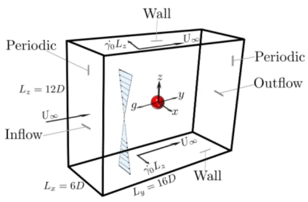
Figure 1: Computational domain and boundary conditions
particle stability in the sheared yield stress fluid. Ovarlez et al. (2012) examined the settling rate of suspensions of particles in different yield stress fluids (concentrated emulsions and Carbopol gels). The density mismatched suspensions are sheared in a wide-gap Couette device; the velocity profile and solid volume fraction are measured by employing magnetic resonance imaging techniques. It is found that, for all the systems, the particles that were stable at rest start sedimenting in the yielded zone as the shear is introduced. Moreover, the experimental results of Ovarlez et al.(2012) show that the particle settling velocity scaled by the Stokes velocity is an increasing function of the inverse Bingham number. Despite all the experimental results falling into a master curve in the limits of high Bingham number (plastic regime), there exists a discrepancy when Bi61, which might be due to another governing dimensionless number associated with the presence of elasticity in a practical yield stress fluid.
A larger number of studies focuses on the effect of shear flow on the particle settling rate in viscoelastic fluids through experimental measurements (see e.g. Van den Brule &
Gheissary 1993; Murchet al. 2017), direct numerical simulations (see e.g. Padhy et al.
2013b,a; Murchet al.2017), and theoretical analysis (see e.g. Brunn 1977b,a; Housiadas
& Tanner 2012; Vishnampet & Saintillan 2012; Housiadas & Tanner 2014; Housiadas 2014; Einarsson & Mehlig 2017).
The drag enhancement on the sphere when it is subjected to an externally imposed cross shear flow is verified through direct numerical simulations both in a weakly (Padhy et al.2013b) and in a highly (Murchet al.2017) constant-viscosity viscoelastic fluid. In the case of weakly viscoelastic fluids, it has been shown that adding polymers indirectly increases the drag on the sphere through breaking the symmetry in the polymer and viscous stresses on the sphere surface (Padhy et al. 2013b). Contrary to the weakly viscoelastic fluids, the form drag is a primary cause of the drag enhancement on the particle in the limit of highly viscoelastic fluids when the cross shear flow is coupled with the uniform flow (Murchet al.2017). In addition to the elasticity effects, the sphere drag coefficient is also affected by the rheological properties of the viscoelastic fluid such as the degree of shear-thinning and the ratio of polymer to total viscosity (Padhy et al.
2013a).
The main novel contributions of our study can be summarised as follows. First, we validate a new tool for the 3D numerical simulations of a sphere settling in a quiescent and sheared yield stress fluid at small particle Reynolds number. We formulate the problem using both an ideal yield stress fluid law (Bingham model) and EVP fluid law.
The governing equations are solved using our recently developed 3D numerical solver to handle the problems including rigid and deformable particles suspended in complex
fluids (Izbassarov et al. 2018). The particle motion in the flow is simulated by means of an efficient Immersed Boundary Method (IBM) coupled with a flow solver for the equations of motions associated with the suspending complex fluids. The mechanical and mathematical modeling, the computational matrix, the boundary conditions, and the numerical scheme of the simulations presented here are reported in section 2. Second, we provide for the first time a 3D and extensive analysis of the velocity, stress fields and yield surfaces around a sphere settling in yield stress fluids. We consider both quiescent and sheared yield stress fluids and compute the drag force and its individual components, i.e., form drag, viscous drag, polymer drag and inertia drag and discuss their dependency on the elastic and plastic properties of the suspending fluids as well as the flow dynamics.
Third, we show that the flow dynamics and drag forces significantly change when a secondary linear cross shear flow is superimposed. In particular, the nonlinear coupling of the settling and simple shear flow plays a significant role in determining the flow dynamics and consequently the drag force on the sphere, which makes the prediction of sphere drag in a sheared yield-stress fluid difficult (section 3). The main conclusions of this work are summarized in section 4.
2. Problem definition
2.1. Problem definition
We consider the sedimentation of a single spherical particle subjected to a linear cross shear flow in an EVP fluid with slight inertia. The reference frame is attached to the particle with its origin at the particle center. Thus, the particle remains stationary and the fluid moves with uniform velocityU∞in the opposite direction of gravity (Figure 1).
The top and bottom walls are translating with constant and equal velocity, but in the opposite direction to create the linear shear flow in the xz plane. Moreover, the walls move with the uniform velocity U∞ in the streamwise direction y. Consequently, the upper and lower plates are moving obliquely. While remaining fixed, the particle rotates freely due to the applied cross shear flow.
2.2. Mechanical model of EVP material
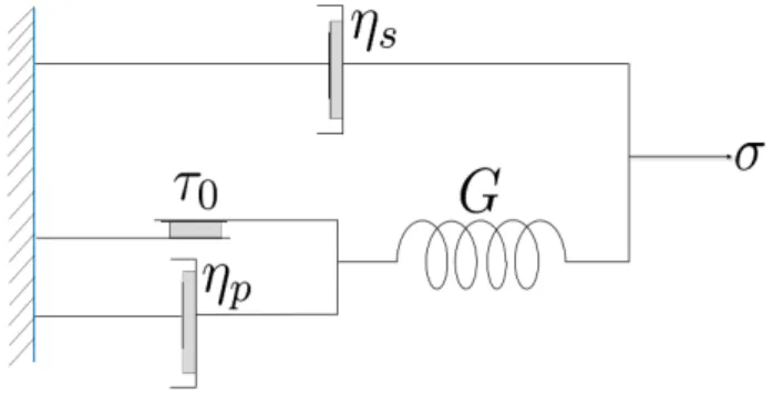
In this paper, we have adopted the model proposed by Saramito (2009) to simulate the EVP material. Figure 2 represents a mechanical description of this model, based on the frictionτ0, spring stiffnessGand solventηsand polymerηp viscosities. When the elastic strain energy of the system exceeds the threshold value (yield value), the friction element breaks allowing viscous deformation. After yielding, the deformation is unbounded in time, thus the system behaves as a non-linear viscoelastic fluid. Before yielding, however, the material behaves as a non-linear viscoelastic solid.
2.3. Mathematical model
This section presents the governing equations in dimensionless form. Here, the charac- teristic velocity scale is the uniform inflow velocityU∞, the characteristic length scale is the particle diameterD, the characteristic time scale isD/U∞(since the uniform flow is the main flow), andη0U∞/Dis the characteristic stress.η0is the total viscosity at zero shear-rate which is sum of the solvent ηs and polymer ηp viscositiesη0 =ηs+ηp. The continuity and momentum equations are as follows:
∇.u= 0, (2.1)
Figure 2: Mechanical model schematic of an EVP material proposed by Saramito (2009).
Rep(∂u
∂t +u∇u) =∇.(−pI+ 2(1−β)D(u) +τ) +f, (2.2) where u is the fluid velocity vector andD(u) is the rate of deformation tensor defined as D(u) = 12(∇u+∇uT). It is noteworthy to mention that, we subtract the static pressure of the fluid and scale the remainder with the viscous stress scale. Therefore, the dimensionless pressure p is the dimensionless dynamic pressure. Here, Rep is the particle Reynolds number that is defined as the ratio of the inertial forces to viscous forces;Rep= ρfUη∞D
0 , whereρf is the fluid density. The retardation parameter,β, is the ratio between the polymer and the total viscosities ηp/η0, f is an external body force (IB force) used to model the presence of the particle.τ is the extra stress tensor due to the plasticity and elasticity of the EVP fluid.
The following constitutive equation is proposed to model the stress-deformation of EVP materials (Saramito 2009):
W i∇τ+κn(|τd|)ατ−2βD(u) = 0, (2.3) where W i is the shear Weissenberg number, the ratio of the material relaxation time scale λ to the cross shear flow time scale 1/γ˙0. Therefore, W i = λγ˙0. Note that the material relaxation timeλis the ratio of polymer viscosityηpto the elasticity parameter G; λ = ηp/G. α is another dimensionless parameter whose magnitude determines the primary and secondary flow; in particular, the ratio of the applied shear rate ˙γ0 to the shear rate induced by particle settling in the fluid ˙γsett is denoted byα= ˙γ0/γ˙sett. The settling shear rate is the ratio of the uniform inflow velocity to the particle diameter, i.e,
˙
γsett =U∞/D and thus,α= ˙γ0D/U∞. In the context of EVP fluids, αcan be viewed as the ratio between the shear Weissenberg number W i and the settling Weissenberg number, which is called “W i∞” in the present work and is equal to λUD∞.
∇τ is the upper convected derivative of the stress field; it is computed based on the following relation:
∇τ = ∂τ
∂t +u.∇τ−(∇u)T.τ−τ.∇u. (2.4)
In equation (2.3)κn(|τd|) is the plasticity criterion, defined by the following relation:
κn(|τd|) =max(0, |τd| −Bi
(2β)1−n|τd|n)1n, (2.5)
where|τd|is the second invariant of the deviatoric part of the extra stress tensor:
τd=τ−1
3tr(τ)I, (2.6)
with I the unit tensor and n the power-law index. Bi is the Bingham number, which is the ratio of yield stress to viscous stress, Bi = ητ0D
0U∞. τ0 is the material yield stress.
Note that throughout the paperBiis the Bingham number defined based on the particle settling shear rate. Polymer viscosity is computed via: ηp =κ(UD∞)n−1, where κis the consistency parameter.
The rotational particle velocity is computed by solving the Euler equation in the body- fixed reference frame:
Is
dωc
dt = I
∂Ω
r×(τ.n)dA. (2.7)
In equation 2.7,Isis the moment of inertia of the particle and is equal to25ρsVsR2, where ρs is the particle density, Vs is the particle volume and R is the particle radius. Here, nis the unit normal vector at the particle surface ∂Ω and ωc is the particle rotational velocity. Since our simulations are performed in a body-fixed reference frame, the particle angular velocity is tracked in an inertial reference frame by adopting the rotation matrix from Chenet al.(2006). For more details on the transformation the reader is referred to V´azquez-Quesada et al.(2016).
2.4. Boundary conditions
The computational domain is a rectangular box with length of 16D in the streamwise y direction, 6D in the spanwisexdirection and 12Din the wall-normalzdirection. The particle is located in the middle of the box with its center as the origin of the coordinate system. The inlet velocity boundary condition is a combination of uniform velocity and the simple shear flow. Hence, at the inlet, the fluid velocity has a component in both the streamwise and spanwise directions. The convective outflow boundary condition is applied at the outlet where the fluid is leaving the domain in theydirection. The velocity is extrapolated by solving the convective equation at the location of the outlet (Uhlmann 2003):
∂u
∂t +U∞∂u
∂n = 0. (2.8)
In order to maintain the overall mass balance and satisfy the compatibility condition, the convective velocity should be equal to the uniform inflow velocity U∞. A no slip boundary condition is applied at the top and bottom plates with velocities of the plates equal tou=−γ˙0Lzxˆ+U∞yˆandu= ˙γ0Lzx+Uˆ ∞y. A homogeneous Neumann conditionˆ is used for pressure at the two walls as well as the inlet and outlet (∂p/∂n= 0). A no flux condition is specified normal to the confinement walls for the extra stress tensor. A periodic boundary condition is applied for the velocity, pressure and extra stress tensor in the spanwisexdirection. The no-slip/no-penetration boundary condition is satisfied at the sphere surface implicitly by using the multidirect forcing Immersed-Boundary scheme (Breugem 2012).
We analytically solve the EVP constitutive equations of Saramito (2009) for the combination of Couette and uniform flow at steady state in the absence of the spherical particle and then apply this solution for the EVP stress tensor at the inlet. At steady- state the flow of EVP fluid is entirely yielded. Thus, the plasticity criteria function is positive and non-zero (κn(|τd|)>0). In this flow configuration, all the components of the extra stress tensor are zero except the normal and shear stress in the spanwise direction
Shear-induced sedimentation W i∞ W i β n Rep Bi 0.1,1 0.01,0.1 0.8 1 1 0.05
0.1 0.13
0.5 1
Pure sedimentation 0.1 0 0.8 1 1 0.05
0.1 0.13
0.5 1 Table 1: Computational matrix
of the shear planexz. The non-vanishing value of the normal stress difference, which is observed in practical yield stress fluids (e.g. Janiaud & Graner 2005), is the result of incorporating the elastic stresses in the EVP constitutive equation as the classical visco- plastic models (such as Bingham 1922; Herschel & Bulkley 1926) do not predict the first normal stress difference in shear flows. The analytical solution is obtained by solving the following coupled non-linear equations for the normal and shear EVP stresses:
(|τd| −Bi
|τd| )τxz = 2αβ, (2.9)
τxz = r αβ
2W iτxx, (2.10)
where |τd| = q
1
3τxx2 +τxz2 as τxx and τxz are the only non-zero elements of the stress tensor. The non-linear system of equations (2.9) and (2.10) is easily solved using the fsolve routine of MATLAB. For the pure sedimentation simulations, the stress tensor at the inlet and outlet is set equal to zero.
2.5. Computational matrix
In this study, all the simulations are conducted at α = 0.1, i.e, the particle settling shear rate is ten times larger than the externally imposed shear rate. We will present a series of simulations for the problem of single sphere settling through EVP fluid in the absence and presence of simple cross shear flow. The dimensionless parameters used for the simulations presented here are reported in table 1.
2.6. Numerical Method
The comprehensive details of the numerical algorithm are explained by Izbassarov et al.(2018). In brief, the equations are solved on a Cartesian, staggered, uniform grid with velocities located on the cell faces and all the other variables (pressure, stress and material component properties) at the cell centers. All the spatial derivatives are approximated with second-order centered finite differences except for the advection terms in equation (2.4) where the fifth-order WENO (weighted essentially non-oscillatory) scheme is adopted (Shu 2009). The time integration is performed with a fractional-step method (Kim & Moin 1985), where all the terms in the evolution equations are advanced in time with a third-order explicit Runge-Kutta scheme except for the EVP stress terms which are advanced with the CrankNicolson method. Moreover, a Fast Poisson Solver is
used to enforce the condition of zero divergence for the velocity field. The coupling of the fluid and particles is performed with the immersed boundary method proposed by Breugem (2012).
We have adopted a grid resolution of 32 Eulerian grid points for particle diameter. Each simulation is performed on 128 cores working in parallel and the steady-state solution is obtained after approximately 16 weeks, corresponding to approximately 2600 CPU hours.
2.7. Code validation
The present three-dimensional numerical solver has been used and extensively validated in the past for particulate flows (Lashgari et al. 2014), non-Netwonian flows (Rosti
& Brandt 2017; Alghalibi et al. 2018; Rosti et al. 2018; Shahmardi et al. 2019), and multiphase problems in non-Newtonian fluids (De Vita et al. 2018). In particular, the code is recently validated for suspensions of rigid and soft particles and droplets in EVP and viscoelastic fluids (Izbassarov et al. 2018). Nonetheless, we report here a further validation case for a simple shear flow of EVP fluid at different power law indexesn.
2.7.1. EVP Couette flow
We consider the two-dimensional shear flow (Couette flow) of an EVP fluid. Initially, the material is at rest and starts flowing due to an externally applied constant shear rate
˙
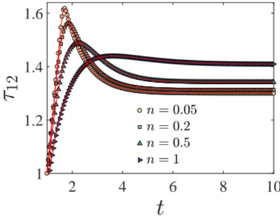
γ0. The objective here is to track the time evolution of the shear stress (τ12, with 1 and 2 being the streamwise and wall-normal directions respectively) for different values of the power-law indexnand compare them with the analytical solution provided by Saramito (2009).
The shear Weissenberg number is fixed to W i = 1, the Bingham number Bi = 1 and the retardation parameterβ = 1. The simulations are performed for the power-law index range 0.056n61. The time evolution of the shear stressτ12and the comparison with Saramito (2009) are depicted in figure 3. We observe that, initially, the shear stress grows linearly, but as soon as the stress level achieves a threshold value, which is called
“yield stress”, the growth stops and a plateau is reached; this is expected in the yielded state. Indeed as soon as the second invariant of the deviatoric stress tensor exceeds the material yield stress (orBinumber in dimensionless context), the plasticity criteria functionκn(|τd|) becomes positive and non-zero in the constitutive equation precluding the stress growth. Consequently, the solution remains bounded for any positive value of the power-law index. As shown in the figure, we find a very good agreement with the results by Saramito (2009).
3. Results and discussion
In this section, we first present the results of the pure sedimentation simulations, i.e, in the absence of any external shear flow, and then those of the shear-induced sedimentation, i.e, from the simulations involving cross shear flow.
3.1. Pure sedimentation in EVP fluids
For the case of a sphere settling in an EVP fluid in the absence of cross shear flow, the dimensionless numbers have been chosen in such a way that the gravity number (related to Bingham number; Yg, see equation 3.1) remains smaller than its critical valueYgc reported by Fraggedakis et al.(2016a). Above the critical condition the yield stress resistance overcomes the buoyancy force and, consequently, the particle is trapped
2 4 6 8 10 1
1.2 1.4 1.6
Figure 3: Time evolution of shear stress in a stationary simple Couette flow. The solid lines and symbols represent the analytical solution given by Saramito (2009) and the present numerical simulations, respectively.
W i∞ Bi De Yg Ygc(eqn: 3.2) 0.1 0.05 1.31 0.0071 0.1426
0.1 1.46 0.0128 0.1554 0.13 1.53 0.0159 0.1614 0.5 2.07 0.0453 0.2017 1 2.47 0.0758 0.2289
Table 2: Dimensionless numbers of the pure sedimentation simulations with associated gravity numberYg, smaller than its critical valueYgc.
inside the yield-sress fluid. The critical gravity number is found to be Ygc = 0.143 for Bingham fluids (i.e. in the absence of elasticity) by Beriset al.(1985). However, numerical simulations have demonstrated that this value increases with the material elasticity.
Here, we show that the gravity numbers for the current simulations are smaller than the critical gravity number presented as the stoppage criteria by Fraggedakiset al.(2016a).
To this end, we must first rescale our parameters following their definition. Thus, for each simulation we must find the corresponding Deborah number, De, and gravity number, Yg, defined as:
De=λ∆ρgR ηp
; Yg= 1.5 τ0
∆ρgR, (3.1)
where ∆ρ is the density difference between the bead and the fluid. The critical gravity number is obtained using non-linear regression on the simulation data in Fraggedakis et al.(2016a):
1
Ygc = 1.2 + 1
0.176 + 0.135De. (3.2)
The parameters of the simulations, including the Deborah and gravity numbers, and the comparison with the critical gravity number predicted by equation (3.2) are shown in table 2. According to this table, the gravity number in the present work is always smaller than its critical value.
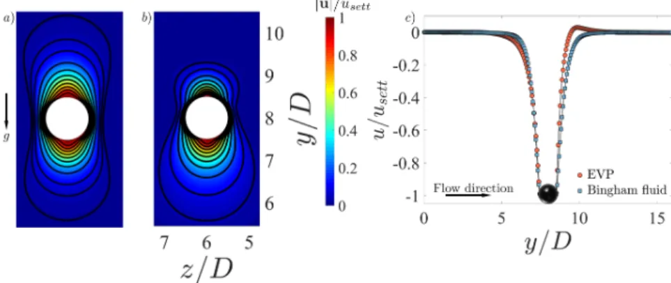
Figure 4: a) Normalized velocity magnitude around the particle settling in the yz centerplane (x = 3D) through Bingham fluid and b) EVP material at W i∞ = 0.1. c) Streamwise velocity around a particle settling in a Bingham fluid and an EVP material at the channel center line (x= 3D,z= 6D). In all figures, the Bingham numberBi= 0.5.
3.1.1. Velocity and stress fields
In this section the velocity and stress fields around a sphere are demonstrated to show the effects of elasticity and plasticity on the flow dynamics. To better highlight the elasticity effects on the flow features and the sphere drag, we have performed the additional simulations of particle settling in a Bingham fluid, whose details are presented in Appendix A.
Figure 4 shows the contour plot of the velocity magnitude in the midyzplane around the surface of the particle settling in an otherwise quiescent EVP fluid. An analogous map for the Bingham fluid is included for the sake of comparison (see methods and details in Appendix A). The Bi number is held fixed and equal to 0.5 for both cases and the settling Weissenberg number W i∞ = 0.1 for the EVP material and 0 for the Bingham fluid. The magnitude of the velocity is normalized by the particle settling velocity,usett. Note that we depict the flow only in a small window around the particle to highlight the shape of the velocity contours.
We observe that, the symmetry of the velocity field around the particle stagnation points (north and south poles of the sphere) is broken and an overshoot in the downstream velocity appears as soon as a small elasticity (W i∞= 0.1) is added to the carrying fluid.
This behavior is quantitatively depicted in figure 4c), where the normalized streamwise velocity is plotted in the flow direction at the center line of the channel, i.e, as function ofy forx= 3D,z= 6D.
The loss of the fore-aft symmetry in a yield stress fluid and the negative wake formation have been previously observed in experiments (Gueslin et al. 2006; Putz et al. 2008;
Holenberg et al. 2012; Ahonguio et al. 2014). Fraggedakis et al. (2016a) revealed that the elasticity of realistic yield stress fluids is the primary cause of such phenomena.
Indeed, these authors demonstrated that the thixotropy (aging of yield stress materials) is not responsible for such behavior as conjectured before. The absence of this symmetry was also observed in the case of a neutrally-buoyant sphere in Carbopol gels subjected to simple shear flow (Firouzniaet al.2018). Therefore, to correctly predict the behavior of practical yield stress fluids, the effect of elasticity should be taken into account. It is also worthwhile to mention that the loss of the fore-aft symmetry is not due to the weak inertia of our simulations (Rep= 1), see section 3.1.3 for an explanation.
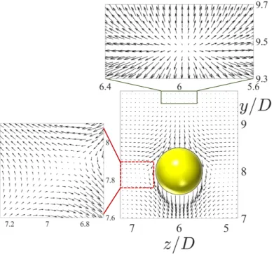
The velocity vector field around the particle settling in an EVP fluid is illustrated in
Figure 5: Velocity vectors around the sphere settling in an EVP material in the central yzplane. The dashed red and solid green boxes magnify the recirculation zones and the flow stagnation points. The dimensionless numbers are the same as figure 4.
figure 5 for the same case as in figure 4. For clarity, the recirculation zones (inside of the dashed red box) and flow stagnation points (from the solid green box) are magnified.
The negative wake is observed where the fluid velocity is opposite the particle velocity, upstream of the rear stagnation point. The overshoot in the stream velocity downstream of the particle shown in figure 4c) occurs in the same area. For a particle with no-slip boundary condition, the recirculation zones arise close to the particle and in its equatorial plane as previously observed experimentally (Holenberget al.2012), which could also be captured computationally by adopting an extensive mesh refinement near the particle surface (Fraggedakiset al. 2016a).
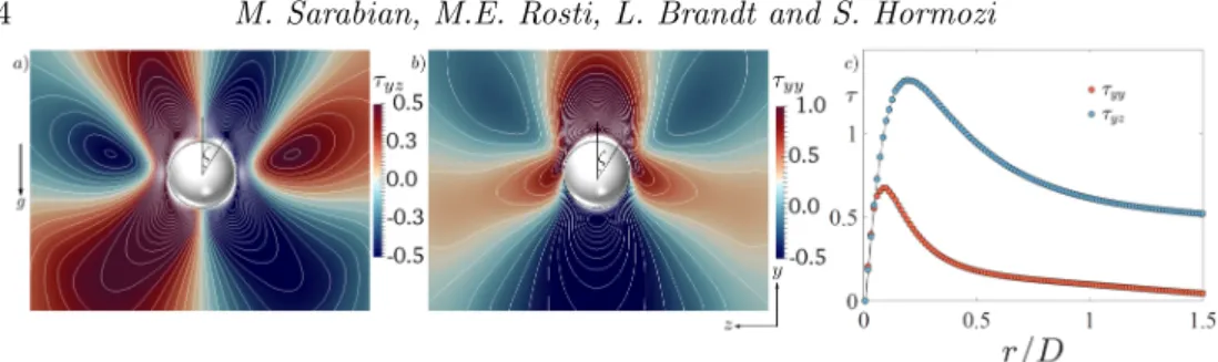
The interaction between shear and normal stresses upstream of the particle is shown to be the main cause for the negative wake formation (Fraggedakiset al.2016a). Infact, the negative wake is due to the normal stress relaxing faster than the shear stress away from the particle. This is shown in the colormap of normal and shear stresses around the sphere in figures 6a) andb). The stress relaxation away from the sphere, in particular the shear and normal stresses, are also depicted along the ray at an angleζ= 30◦, measured from the rear stagnation point (sphere north pole) in figure 6c) (we define the north pole in the positive ydirection).
Clearly, at r ≈ 0.2D, the absolute value of the shear stress is twice as large as the normal stress. Thus, the elastic shear stress, which is responsible for the creation of a rotational force on the fluid element, contributes to the negative wake and to the secondary flow upstream of the particle. For more details the reader is referred to Fraggedakiset al.(2016a).
Figure 6: Stress fields around the particle settling in an EVP fluid in the yz plane at x= 3D a) theτyzshear stress andb) theτyy normal stress. The angleζis measured from the north pole of the sphere.c) Stress relaxation versus the distance from the particle, r, at an angleζ= 30◦ measured from the north pole of the sphere.r= 0 corresponds to the particle surface. The absolute value of the stresses are shown for the same case as in figure 4.
3.1.2. Yielded/unyielded regions
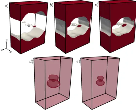
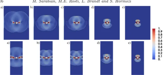
In this section, we show the shape and extent of the yielded/unyielded zones around a sphere at different Binumbers in an EVP material. To our knowledge, the unyielded regions have not been previously reported in 3D. Figure 7 displays the surfaces delimiting the yieldied regions at differentBinumbers and constant elasticity (W i∞= 0.1), where unyielded surfaces are plotted with lower transparency for higher Bi numbers (Bi = 0.5,1) for the sake of clarity. In the figure, red represents the unyielded regions, while gray depicts the yielded surface boundary and the particle. For completeness, figure 8 shows the projection of unyielded surfaces onto the midyzandxyplanes. In this figure, blue and gray colors denote the yielded and unyielded zones respectively.
The simulations reveal the existence of two unyielded zones; the first is the unyielded envelope that surrounds the fluid zone; the second is the unyielded ring located in the yielded zone surrounding the sphere. The projection of this ring in the central yz and xyplanes is shown in figure 8. These are the two unyielded islands in the yielded region located at the equator and on either side of the sphere. It is noteworthy to mention that these solid islands are the regions in which the second invariant of the shear rate is almost zero as shown in figure 9. Therefore, unlike the case of 2D cylinders, these solid rings are not rotating solid islands; note also that, at steady state, the sphere rotating velocity is zero in the pure sedimentation cases.
We note that the outer unyielded envelope grows progressively as the Bi number increases and the yield surface boundary approaches the surface of the particle from the equator plane causing the particle to stop settling. A similar arrest mechanism has been captured previously in axisymmetric particle-settling simulations in an EVP material (Fraggedakis et al. 2016a). Moreover, figure 8 shows that there exists yielded regions in the vicinity of the channel walls for Bi = 0.1&0.13. These are associated with the wall effects and had also previously been observed by Blackery & Mitsoulis (1997) in the Bingham fluid flow past a sphere contained in a tube with a diameter that is 10 times larger than that of the sphere.
3.1.3. Drag coefficients
In our simulations we fix the particle and compute the drag exerted on the particle by the surrounding fluid. Since the settling rate is inversely proportional to the drag, drag enhancement is equivalent to settling rate reduction (Padhyet al.2013b). The drag
Figure 7: Surfaces of unyielded regions around the particle in an EVP material atW i∞= 0.1 in the absence of cross shear flow for variousBi;a)Bi= 0.05b)Bi= 0.1c)Bi= 0.13 d)Bi = 0.5 e)Bi = 1. Red represents the unyielded zone, while gray shows the yield surface boundary.
Figure 8: Evolution of the unyielded zones for flow of an EVP material around a particle for various Bi numbers atW i∞ = 0.1;a)Bi = 0.05b)Bi= 0.1 c)Bi= 0.13 d)Bi= 0.5 e)Bi= 1. The first and second row represents the unyielded zones in the centralyz and xyplanes respectively. Blue and gray represent the yielded and unyielded regions.
Figure 9: Colormaps of the second invariant of the shear rate for the flow of an EVP material around a particle for various Bi numbers at W i∞ = 0.1; a) Bi = 0.05 b) Bi= 0.1 c)Bi= 0.13 d)Bi = 0.5 e)Bi= 1. The first and second row represents the shear rate in the centralyzandxyplanes, respectively.
coefficientCd is defined as follows:
Cd= 2Fd
η0U∞D, (3.3)
whereFd is the total drag force exerted on the particle in the streamwise (y) direction.
To investigate the dependency of the drag change on the flow and fluid parameters, we decompose the total drag force on the particle into its individual components, which are associated with the different stress contributions. As we assume a finite particle Reynolds number (Rep= 1), the total drag consists of four components; namelyform drag (Fdf), viscous drag (Fdv), polymer drag (Fdp) andinertia drag (FdI). The different components are computed from the following definitions:
Fdf=− ZZ
∂Ω
pnydS, (3.4)
Fdv= (1−β) ZZ
∂Ω
(∂uy
∂xj
+∂uj
∂y )njdS, (3.5)
Fdp= ZZ
∂Ω
τyjnjdS, (3.6)
FdI =Rep
ZZ
∂Ω
uj
∂uy
∂xj
njdS, (3.7)
where∂Ω is non-dimensionalized byD2. The details of the numerical integration proce- dure are given in appendix B.
The form drag (eq. 3.4) is the drag component resulting from the distribution of the dynamic pressure on the sphere. It is noteworthy to mention that in the Saramito’s model (Saramito 2009) the extra elastic stress tensor is not traceless, i.e, tr (τ) is not zero. Thus, the pressure fieldpobtained in the numerical solution is basically the field of ¯p=p+ 13tr (τ)
. However, in all of our simulations, the absolute value of the 13trτ at the surface of the sphere is negligible when compared to the absolute value of ¯p= p+ 13trτ
. In addition, unlike ¯p, the sign of 13trτ
does not change at the stagnation
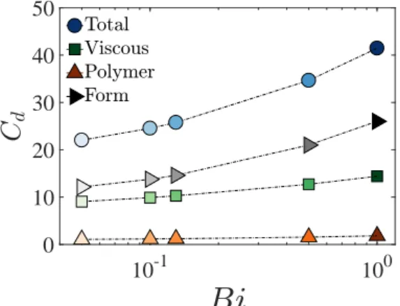
10-1 100 0
10 20 30 40 50
Figure 10: Total drag coefficient and its individual components for a sphere settling in an EVP fluid as a function of theBi number atW i∞= 0.1.
points. Therefore, we conclude that the contribution of 13trτ
to the drag is negligible as compared to the contribution of the dynamic pressure field p for the simulations conducted in this work.
To significantly reduce the time of each computations, we have assumed small but finite inertia, Rep = 1, and still expect inertial effects to be negligible. To a posteriori check this, we have compared the sum of the form, viscous and polymer drag force to the IB forcefj, i.e. the total drag, and found a difference of about 1.5%, which indeed indicates negligible inertial drag,FdI.
Figure 10 illustrates the variation of the total drag coefficient and its individual contributions (form, viscous and polymer drag) experienced by the sphere settling in an EVP fluid as a function of the Bi number. The total drag increases as the material yield stress is increased, as observed in the past for the particle settling in a purely visco-plastic fluid (Beris et al. 1985; Atapattu et al. 1995; Blackery & Mitsoulis 1997;
Tabuteau et al. 2007; Holenberg et al. 2012; Ahonguio et al. 2014; Wachs & Frigaard 2016) as well as in an EVP fluid (Fraggedakiset al.2016a). Here, the key finding of our 3D simulations is that the drag contribution from the dynamic pressure distribution on the particle (form drag) is dominant. Additionally, the viscous drag increases with Bi, whereas the drag contribution due to the polymer stresses remains almost constant with Bi.
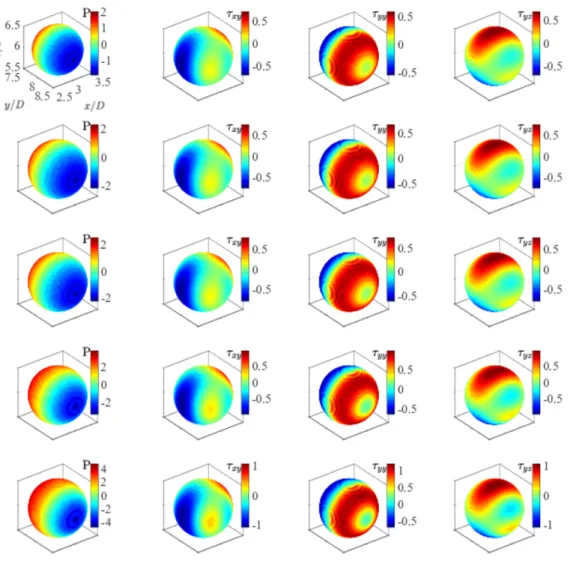
The dynamic pressure and of the three components of the viscous stress distribution (τxy, τyy, τyz) are computed on the surface of the sphere and are shown in figure 11 (the computational procedure is explained in details in appendix B). Note that in this study we are dealing with a complex flow, i.e. the type of flow is in general different at each point, e.g. predominantly shear, extensional, nearly rigid-body motion or a combination of these. However, our goal is to show the components of the stress that contribute to the drag force, i.e., Fi =R
∂Ωτij.nj dA. For a drag force in they direction, the relevant components of the stress tensor areτyx, τyyandτyz, so we just examine these components of the viscous stress tensor, since figure 10 shows the polymer stress contribution to the drag force is negligibile.
The visualizations in figure 11 confirm that the magnitude of the pressure on the particle surface increases withBi. Moreover, the fore-aft symmetry in the pressure distri- bution around the particle stagnation points breaks leading to further drag enhancement.
Increasing the Bingham number, on the other hand, merely magnifies the value of the