量子力学第二 レポート課題

量子力学第二 レポート課題

出題日：平成２３年４月１２日（火） 担当：武藤

提出締切：平成２３年５月３１日（火）１２時１０分 提出場所：Ｈ１１１講義室

締切前には本館１階１８９号室でも受け取るが，郵便受けには入れないこと。

Ａ４版のレポート用紙を用い，綴じて提出すること。

レポートには表紙をつけ，表紙には学科，学籍番号，氏名を明記すること。

解答は表紙の次のページから，問題番号順に書くこと。

人と相談するのはよいが，他人のレポートを写してはならない。

添付資料は量子力学の教科書

”Elementary Quantum Mechanics”

Preliminary Edition David S. Saxon Holden-Day, Inc., 1964

の第９章

Motion in Three Dimensions

Motion in Three Dimensions 1 Formulation: Motion of a Free Particle

For reasons of simplicity, we have thus far considered only one-dimensional motion.

We now generalize our treatment to three dimensions. No conceptional difficulties are encountered, as we shall see.

We consider the motion of a particle of mass m in an external potential V (r), where r is the position vector of the particle referred to some conveniently chosen origin. The Hamiltonian for this system is then

H = p ²

2 m + V (r) (1)

where p is the vector momentum of the particle. Introducing a set of unit vectors e x , e y , and e z , along the axes of rectangular coordinates, we have

r = x e _x + y e _y + z e _z ,

p = p _x e _x + p _y e _y + p _z e _z . (2) It is often convenient to use numerical indices to identify the components of vectors, and we shall therefore also write (2) in the equivalent form

r = x ₁ e 1 + x ₂ e 2 + x ₃ e 3 ,

p = p ₁ e 1 + p ₂ e 2 + p ₃ e 3 , (3) where the subscripts 1, 2, 3 are intended to represent the x , y and z components respectively.

Different spatial components of the motion represent different degrees of freedom and hence commute with each other. The general commutation relations can thus be compactly written,

[ p _i , p _j ] = [ x _i , x _j ] = 0 , [ p _i , x _j ] = ¯ h

i δ _ij . (4)

In particular, in configuration space, the x _i are numbers and p _x = ¯ h

i

∂

∂x , p _y = ¯ h i

∂

∂y , p _z = h ¯ i

∂

∂z , whence, introducing

∇ = e x ∂

∂x + e y ∂

∂y + e z ∂

∂z , (5)

we have, in brief,

p = ¯ h

i ∇ . (6)

The wave function ψ (r , t ) = ψ ( x, y, z, t ) satisfies the time dependent Schr¨odinger equation

H ψ = E ψ (7)

where

E = − h ¯ i

∂

∂t

and the Hamiltonian operator, in configuration space, is given by H = 1

2 m

p _x ² + p _y ² + p _z ² + V (r) = − ¯ h ² 2 m

∂ ²

∂x ² + ∂ ²

∂y ² + ∂ ²

∂z ²

+ V (r) or using (5),

H = − ¯ h ²

2 m ∇ ² + V (r) . (8)

The operator ∇ ² is called the Laplacian operator or simply, the Laplacian. In any case, Schr¨odinger equation in configuration space is the partial differential equation,

− ¯ h ²

2 m ∇ ² + V (r)

ψ (r , t ) = − h ¯ i

∂ψ

∂t . (9)

As usual, the stationary state solutions can be separated out by writing

ψ _E (r , t ) = ψ _E (r) e ^{−iEt/¯ h} (10) and we obtain at once the time independent Schr¨odinger equation

− ¯ h ²

2 m ∇ ² + V (r)

ψ _E (r) = E ψ _E (r) . (11) The fact that this is a partial, rather than an ordinary differential equation, as it was in one dimension, is responsible for the greatly increased mathematical complexity of the three-dimensional problem.

Before going on to consider the solutions of equation (11), we remark that for nor- malized wave functions, ψ ^∗ ψ is the probability density in ordinary three space and that expectation values are defined by

ψ | A | ψ = ψ ^∗ (r , t ) A ψ (r , t ) d ³ r (12) where the symbol d ³ r means the three-dimensional volume element. We remark also that the probability flux or current density is given by

j = ¯ h 2 mi

ψ ^∗ ∇ ψ − ψ ∇ ψ ^∗

which is an obvious generalization of equation (VI-87). It is not difficult to verify that

probability is properly conserved.

Finally, we remark that the equations above apply not only to the motion of a particle in an external potential, but equally to the description of the relative motion of a pair of isolated interacting particles (after the uninteresting center of mass motion has been separated out). In the latter case, the coordinate r is the distance between the particles, V (r) in their interaction potential, p their relative momentum and m their reduced mass.

The solutions of equation (11) are rather complicated in general and can only be obtained exactly and explicitly for a few simple cases. The simplest case of all, of course, is that of a free particle, when V (r) vanishes. The free particle solutions are just de Broglie waves travelling in some given direction, and are easily verified to be

ψ

(r) = exp i p · r

¯ h

= exp i ( p _x x + p _y y + p _z z )

¯ h

, E = p ²

2 m (13)

where, as our notation indicates, these are states of definite vector momentum p.

Note that such states are infinitely degenerate since there are infinitely many possible orientations of the momentum vector for a fixed energy E .

The momentum states form a complete set, and hence any wave function can be expressed as a superposition of these functions. We thus have the three-fold Fourier integral representation

ψ (r , t ) = 1 2 π ¯ h

_3/2

d p _x d p _y d p _z φ (p , t ) exp i ( p _x x + p _y y + p _z z )

¯ h

or, in brief,

ψ (r , t ) = 1 2 π h ¯

_3/2

d ³ p φ (p , t ) exp i p · r

¯ h

(14) where, φ (p , t ), the probability amplitude in momentum space, can be expressed in terms of ψ (r , t ) by the inversion,

φ (p , t ) = 1 2 π h ¯

_3/2

d ³ r ψ (r , t ) exp − i p · r

¯ h

. (15)

Equations (14) and (15) are thus seen to be three-dimensional generalization of our earlier results in one dimension.

2 Potentials Separable in Rectangular Coordinates

The simplest three-dimensional problem is that in which the potential has the very special form,

V (r) = V ₁ ( x ) + V ₂ ( y ) + V ₃ ( z ) (16) since in that case Schr¨odinger equation separates in rectangular coordinates, as we now show. The stationary state Schr¨odinger equation for such a potential has the form,

− ¯ h ² 2 m

∂ ²

∂x ² + V ₁ ( x )

+

− ¯ h ² 2 m

∂ ²

∂y ² + V ₂ ( y )

+

− ¯ h ² 2 m

∂ ²

∂z ² + V ₃ ( z )

ψ _E = E ψ _E

and hence, writing

ψ _E ( x, y, z ) = ψ _E

( x ) ψ _E

( y ) ψ _E

( z ) = ψ _E

( x ₁ ) ψ _E

( x ₂ ) ψ _E

( x ₃ ) we obtain, for each factor,

− ¯ h ² 2 m

∂ ²

∂x ² _i + V _i ( x _i )

ψ _E

( x _i ) = E _i ψ _E

( x _i ) , i = 1 , 2 , 3 E = E ₁ + E ₂ + E ₃ .

Thus, the states are a simple composition of familiar one-dimensional states.

As a first example, consider the states in a rectangular box of sides, L ₁ , L ₂ , and L ₃ respectively. Taking the origin to be at one corner of the box we see that if ψ _E is required to vanish at each of the walls, then the stationary state solutions are

ψ _E =

8

V sin n ₁ πx

L ₁ sin n ₂ πy

L ₂ sin n ₃ πz

L ₃ , n _i = 1 , 2 , 3 , · · · where V = L ₁ L ₂ L ₃ is the volume of the box and

E = ¯ h ² 2 m

n ₁ π L ₁

₂

+ n ₂ π L ₂

₂

+ n ₃ π L ₃

₂

= E _n

_n

_n

.

The spectrum is thus fairly complicated and has no particular regularities for general L ₁ , L ₂ , and L ₃ .

For a cubical box the situation is somewhat simpler since in that case, E _n

_n

_n

= ¯ h ² π ²

2 mL ²

n ₁ ² + n ₂ ² + n ₃ ² .

The lowest state is that for which n ₁ = n ₂ = n ₃ = 1 and its energy is E ₀ = 3¯ h ² π ² / (2 mL ² ). The next state is that for which one of the n _i is two and the re- maining pair are each unity. Thus this state is three-fold degenerate and its energy is 6¯ h ² π ² / (2 mL ² ) = 2 E ₀ . The third state is that for which any two of the n _i are two and the remaining one is unity. It is also three-fold degenerate and its energy is 3 E ₀ . This regular pattern is broken with the fourth state which occurs when one of the n _i is equal to three and the remaining pair are each equal to unity. This state has energy 11¯ h ² π ² / (2 mL ² ) = 11 E ₀ / 3 and it is three-fold degenerate. The fifth state, which is non-degenerate and has energy 4 E ₀ , occurs for n ₁ = n ₂ = n ₃ = 2, while the sixth state has energy 14 E ₀ / 3 and is six-fold degenerate corresonding to the permutations of its quantum numbers 1 , 2 , and 3. The spectrum obtained in this way is shown in Figure 1.

It is also of interest to consider periodic boundary conditions for the cubical box, that is, boundary conditions which require that ψ _E take on the same value on any pair of opposite walls of the box. For this case,

ψ _E = √ 1

V exp 2 iπ ( n ₁ x + n ₂ y + n ₃ z ) L

Energy in units of E 0

0.0 1.0 2.0 3.0 4.0 5.0 6.0

Quantum numbers ( ) n ₁ n ₂ n ₃ Degeneracy

111 1

211,121,112 3

221,212,122 3

311,131,113 3

222 1

321,312,231,213,123,132 6

322,232,223 3

411,414,144 3

Figure 1: Energies, quantum numbers and degeneracies of the states of a particle in a cubical box. The energy E ₀ of the ground state is 3¯ h ² π ² / 2 mL ² . where

E = E _n

_n

_n

= 2¯ h ² π ² mL ²

n ₁ ² + n ₂ ² + n ₃ ² , n _i = 0 ± 1 , ±2 , · · · . (17) By computing the total number of states N ( E ) of energy less than or equal to E , one can find the density of states ρ ( E ), jsut as we did in one dimension. It is not hard to show in this way that

ρ ( E ) = (2 m ) ^3/2 4 π ² ¯ h ³ V √

E (18)

which is a very useful and important result.

As a second example, we now consider the three-dimensional isotropic harmonic oscillator, described by the potential,

V (r) = 1

2 mω ² r ² = 1

2 mω ² ( x ² + y ² + z ² ) .

This potential is thus of the form of equation (16) and the stationary state solutions of Schr¨odinger equation have the form

ψ _n

_n

_n

= ψ _n

( x ) ψ _n

( y ) ψ _n

( z ) E _n

_n

_n

= n ₁ + n ₂ + n ₃ + ³ ₂ ¯ hω

n _i = 0 , 1 , 2 , · · · ,

(19)

where ψ _n

( x _i ) is the one-dimensional harmonic oscillator stationary wave functions.

The ground state, with energy 3¯ hω/ 2 is not degenerate, but all the remaining states

are, and increasingly so as their energy increases. For example, the first excited state

has energy 5¯ hω/ 2 and is three-fold degenerate (any one of the n _i can be unity, the other two are zero), the second excited state has energy 7¯ hω/ 2 and is six-fold degenerate (any n _i can be two, the others being zero, or any two can be unity, the remaining one being zero). It can be shown that the state of energy ( n + 3 / 2)¯ hω is [( n + 1)( n + 2) / 2]-fold degenerate, this being the number of ways n can be expressed as the sum of three non-negative integers.

3 Central Potentials; Angular Momentum States

We now consider the important case of motion in a spherically symmetric potential, such as the Coulomb potential between point charges, or the gravitational potential between point masses. Such a potential depends, of course, only on the magnitude, and not on the orientation, of the radius vector from a fixed point, which we shall take to be the origin. To describe motion in a potential of this kind, it is convenient to introduce spherical coordinates, r , θ , φ which are defined as follows. Consider a point P with coordinates x , y , z in some right-handed rectangular system. The displacement vector of P relative to the origin is then

r = e x x + e y y + e z z

where e _x , e _y , and e _z are unit vectors along the x , y , and z axes respectively. θ is then defined as the angle between r and the z -axis while φ is defined as the angle between the projection of r in the x - y plane and the x -axis measured clock-wise when looking toward positive z . The range of φ is taken to be zero to 2 π , of θ to be from zero to π . The radial coordinate r is, of course, the magnitude of r and its range is zero to infinity. The relationship between the spherical and rectangular coordinates of P is

x = r sin θ cos φ r = √

x ² + y ² + z ² y = r sin θ sin φ tan φ = y

x

z = r cos θ cos θ = z

√ x ² + y ² + z ² .

(20)

The coordinate system thus defined is clearly orthogonal, and the volume element can be shown to be

d ³ r = r ² d r sin θ d θ d φ.

The element of area on a unit sphere, or element of solid angle, is commonly denoted by d Ω and is given by

d Ω = sin θ d θ d φ (21)

whence also

d ³ r = r ² d r d Ω. (22)

We now seek to write Schr¨odinger equation

− ¯ h ²

2 m ∇ ² ψ _E + V ( r ) ψ _E = Eψ _E (23)

in spherical coordinates. This requires that we express the Laplacian operator ∇ ² in these coordinates. Now, form equation (20), we have

∂

∂x = ∂r

∂x

∂

∂r + ∂θ

∂x

∂

∂θ + ∂φ

∂x

∂

∂φ

= x

r

∂

∂r + xz r ³ sin θ

∂

∂θ − y cos ² φ x ²

∂

∂φ

= sin θ cos φ ∂

∂r + cos θ cos φ r

∂

∂θ − sin φ r sin θ

∂

∂φ with similar complicated expressions for ∂/∂y and ∂/∂z . Recalling that

∇ ² = ∂ ²

∂x ² + ∂ ²

∂y ² + ∂ ²

∂z ² ,

we eventually find, on putting all this together, that (23) becomes,

− ¯ h ² 2 m

1 r ²

∂

∂r

r ² ∂ψ _E

∂r

+ 1

r ² sin θ

∂

∂θ

∂ψ _E

∂θ

+ 1

r ² sin ² θ

∂ ² ψ _E

∂φ ²

+ V ψ _E = E ψ _E (24) which is the desired expression of Schr¨odinger equation in spherical coordinates. In spite of its complicated appearance, this equation is separable as we now proceed to show.

We first separate the angular and radial coordinates by writing

ψ _E ( r, θ, φ ) = R ( r ) Y ( θ, φ ) . (25) After multiplying through by −2 mr ² / ¯ h ² , we then obtain in the usual way

1 Y

1 sin θ

∂

∂θ

sin θ ∂Y

∂θ

+ 1

sin ² θ

∂ ² Y

∂φ ²

= − β 1

R

d d r

r ² d R d r

+ r ² 2 m

¯

h ² [ E − V ( r ) ] R

= β

(26)

where β is the separation constant. The first of these equations can now in turn be separated by writing

Y ( θ, φ ) = Θ ( θ ) Φ ( φ ) .

Multiplying through by sin ² θ , we then obtain, again in the usual way, 1

Φ d ² Φ

d φ ² = − α ² (27)

and 1

Θ

sin θ d d θ

sin θ d Θ d θ

+ β sin ² θ Θ

= α ² (28)

where α ² is a second separation constant. Observe the striking fact that the angular

equations are independent of the potential V ( r ) and of the energy E . The angular

functions are thus universal functions which appear for any central potential. Now it turns out, as we show in a moment, that first equation of (26) defines states of defi- nite angular momentum. If we temporarily accept this assertion, and if we recall that angular momentum is a constant of the motion for a central potential, this behavior is not too surprising. It simply expresses the fact that the states in a central poten- tial involve a universal set of functions characterizing the equally universal angular momentum states of the system.

We now show that the first equation of (26) indeed defines states of definite angular momentum, as asserted. Recall that, with respect to some fixed point which we take to be the origin, the classical angular momentum vector L is given by

L = r × p .

Quantum mechanically, L is taken to be the same function of the quantum mechan- ical dynamical variables, and hence is a vector operator. In configuration space its rectangular components are explicitly,

L _x = yp _z − zp _y = ¯ h i

y ∂

∂z − z ∂

∂y

L _y = zp _x − xp _z = ¯ h i

z ∂

∂x − x ∂

∂z

L _z = xp _y − yp _x = ¯ h i

x ∂

∂y − y ∂

∂x

.

It is not hard to show that in spherical coordinates these rectangular components become,

L _x = − ¯ h i

sin φ ∂

∂θ + cot θ cos φ ∂

∂φ

L _y = ¯ h i

cos φ ∂

∂θ − cot θ sin φ ∂

∂φ

L _z = ¯ h i

∂

∂φ

and hence also, after some more algebra, that L ² = L _x ² + L _y ² + L _z ² = − ¯ h ²

1 sin θ

∂

∂θ sin θ ∂

∂θ + 1 sin ² θ

∂ ²

∂φ ²

.

We thus see that the first equation of (26) is equivalent to L ² Y = β ¯ h ² Y

and hence that, as was to be proved, Y defines a state in which the magnitude of the angular momentum has a definite value, namely √

β h ¯ . We defer a detailed discussion of the subject of angular momentum and its properties to Chapter X. However, before going on, we remark briefly on the orientation of the angular momentum vector. Note that, since L _z = (¯ h/i ) ∂/∂φ , equation (27) is equivalent to

L _z ² Φ = α ² ¯ h ² Φ.

This means that Y = ΘΦ is also an eigenfunction of L _z , with eigenvalue α ¯ h . Thus the angular momentum states Y are states in which the magnitude of the angular momentum vector and its projection on the z -axis are both fixed, with β determining the magnitude and α the projection.

We now turn to the specific angular functions defined by the differential equations (27) and (28). Unfortunately, the latter of these functions is rather complicated. How- ever, for our present purposes, its detailed structure is not particularly relevant. Def- fering a derivation until Chapter X, we shall therefore simply write down the answer.

It turns out that single-valued well-behaved solutions of equations (27) and (28) are obtained only if β and α are such that

β = ( + 1) , = 0 , 1 , 2 , · · ·

α = m, m = 0 , ±1 , · · · , ± . (29) Note that must be a nonnegative integer and that, for a given , m can take on only those integral values which range from − to .

The normalized solution Y ( θ, φ ) = Θ ( θ ) Φ ( φ ), which we denote by Y _m ( θ, φ ) for a particular value of and m , is usually expressed as

Y _m ( θ, φ ) =

2 + 1

4 π P ^m ( θ ) e ^imφ (30)

where the function P ^m ( θ ) = P ^−m ( θ ) is known as an associated Legendre polynomial.

It is a product of sin ^|m| θ and a polynomial of degree − | m | in cos θ , in even powers if − | m | is even, in odd power if − | m | is odd. For reference, the first few Y _m are given below.

= 0 = 1 = 2

m = 0 Y ₀₀ = √ 1

4 π Y ₁₀ =

3

4 π cos θ Y ₂₀ =

5 4 π

3 cos ² θ − 1 2

m = ±1 Y _1±1 =

3

8 π sin θ e ^±iφ Y _2±1 =

5

24 π 3 sin θ cos θ e ^±iφ

m = ±2 Y _2±2 =

5

96 π 3 sin ² θ e ^±2iφ

The normalized angular momentum eigenfunctions are known mathematically as spherical harmonics. They form a complete orthogonal set on a unit sphere. By orthonormality for these functions, we mean that

Y _m ^∗ ( θ, φ ) Y

m

( θ, φ ) d Ω = ^π

0

_2π

0 Y _m ^∗ Y

m

sin θ d θ d φ = δ

δ _mm

(31)

as may readily be verified for any of the particular examples given above.

Although, as we have said, we shall defer a derivation of any of the above features until Chapter X, where we will use a factorization method to construct the solutions, it is instructive to at least indicate how equations (27) and (28) can be handled directly.

The first is trivial; it yields at once Φ ( φ ) = e ^iαφ . Since φ = 0 and φ = 2 π refer to the same point in space, α must be an integer, say m , if Φ is to be a single-valued function.

Equation (28) is more complicated, but it can be solved by a power series method in which Θ is expressed in the form

Θ = sin ^|m| θ

p

c _p cos ^p θ.

It turns out that this series diverges at θ = 0 and π , unless it terminates. The condition that it do so for given m is that β = ( + 1) with − m restricted to nonnegative integral values. The resulting polynomials are the associated Legendre polynomials and the conditions on α and β are those of equation (29).

Thus far we have considered only the angular dependence of the stationary state solutions of Schr¨odinger equation. We must next take up equation (26) for the radial function. Expressing β in terms of , and rearranging slightly, this equation becomes,

− ¯ h ² 2 m

1 r ²

d d r

r ² d R _E d r

+

V ( r ) + ¯ h ² ( + 1) 2 mr ²

R _E = ER _E (32) where we have now introduced the subscripts E and to denote the dependence of R on these quantities. Of course, the entire stationary state wave function is expressed as the product

ψ _Em = R _E ( r ) Y _m ( θ, φ ) (33) where we have again introduced appropriate subscripts to make explicit the fact that these are simultaneously states of definite energy ( E ), angular momentum ( ) and z -component of angular momentum ( m ).

Before going on to consider the solutions of equation (32) for particular potentials, we point out some general properties of the stationary states. Our first remark has to do with the degeneracy of the states. Note that R _E does not depend on m , but only on . Hence, we obtain an eigenfunction corresponding to the same energy for each permissible value of m for a given . Since m can take on any integral value running from − to , there are (2 + 1) such values and thus the states in a central potential are intrinsically (2 + 1)-fold degenerate. As we have seen m measures the projection of L on the z -axis and hence it is essentially determined by the orientation of the angular momentum vector. The degeneracy in question is a consequence of the fact that the Hamiltonian is independent of this orientation when the potential is spherically symmetric.

Our second remark has to do with the parity of the states. The parity operator, it is recalled, changes the sign of all coordinates. Thus, by definition, for arbitrary f ,

P f ( x, y, z ) = f (− x, − y, − z ) .

Reference to equation (20), then shows that in spherical coordinates P f ( r, θ, φ ) = f ( r, π − θ, φ ± π ) .

In particular, therefore,

P ψ _Em ( r, θ, φ ) = R _E ( r ) Y _m ( π − θ, φ ± π ) .

Recalling that P ^m ( θ ) is an even or odd function of cos θ , depending on whether − | m | is even or odd, we see that P ^m ( θ ) has parity (−1) ^−|m| while the remaining factor, e ^imφ , in Y _m , has parity (−1) ^m . Hence

P ψ _Em ( r, θ, φ ) = (−1) ψ _Em ( r, θ, φ ) (34) and the states thus have definite parity. The parity is even or odd depending on whether is even or odd, and not at all on m .

Next, we remark on the interpretation of the term ¯ h ² ( + 1) / 2 mr ² which appears in equation (32). Note that this equation describes radial motion in an effective potential V _eff which is the actual potential V ( r ) supplemented by the term in question. As we now show, a similar term appears in the classical equation for the radial motion of a particle in a central potential. In such a potential the classical orbit lies in a plane containing the origin and perpendicular to the constant angular momentum vector L.

The classical radial equation of motion is, of course, m d ² r

d t ² − mω ² r = − d V d r

where ω is the instantaneous angular velocity of the particle in its orbit. Since L = mωr ² is a constant, on eliminating ω the classical equation becomes

m d ² r d t ² − L ²

mr ³ = − d V d r or, equivalently,

m d ² r

d t ² = − d d r

V ( r ) + L ² 2 mr ²

= − d V _eff

d r . (35)

This latter can be regarded as the radial equation of motion in a reference system

rotating with the instantaneous angular velocity ω , and L ² / 2 mr ² as the potential

generated by the so-called coriolis force associated with such a rotating coordinate

system. This potential is commonly referred to as the centrifugal potential. Note that

it is repulsive and that its effect is to keep a particle with large angular momentum

away from the origin. In any case, and independently of the interpretation, comparison

with equation (32) shows that the effective potentials for the classical and quantum

mechanical radial motion have exactly the same form. Indeed, since the eigenvalues of

L ² are ( + 1)¯ h ² , these effective potentials are actually identical.

Finally, we remark on the relation between the radial equation (32) and the by now familiar equation for the stationary states in one rectilinear dimension. To make this relationship apparent, we write the radial part of the wave function R _E in the form

R _E ( r ) = u _E ( r )

r . (36)

Substituting into equation (32) it gives almost at once,

− ¯ h ² 2 m

d ² u _E d r ² +

V ( r ) + ¯ h ² ( + 1) 2 mr ²

u _E = E u _E (37) which is seen to be rather simpler than equation (32) and, more important, is identical to the stationary state Schr¨odinger equation in one rectilinear dimension. However, equation (37) has meaning only for positive values of the coordinate r . Further if R _E is bounded at the origin, then according to equation (36)

u _E ( r = 0) = 0 . (38)

From this we see that the solutions of the radial equations are exactly the same as the odd state solution in the one-dimensional problem of motion in the symmetrical potential V _eff = V (| x |)+¯ h ² ( +1) /x ² , since these odd states automatically vanish at the origin. The even one-dimensional states do not satisfy equation (38) and hence do not appear in the spectrum. All of the one-dimensional techniques we have learned are thus seen to be applicable to the study of motion in three dimension. Note, moreover, that for given , the radial states are unique; there is one and only one simultaneous radial eigenfunction of E and , for continuum states as well as for bound states. However, eigenstates of any given energy in the continuum can always be found for every value of ; and the continuum states in three dimensions are thus infinitely degenerate.

Furthermore, it may happen that even in the discrete part of the spectrum states of different occur which have the same energy. The degeneracy thus introduced, which is an addition to the intrinsic 2 + 1-fold degeneracy discussed earlier for each state of given , is commonly called an accidental degeneracy. This nomenclature is sometimes inappropriate but instead may be consequence of additional symmetries in the Hamiltonian beyond the spherical symmetry we have assume for V ( r ). We shall shortly present some examples which illustrate this behavior. The above remarks are perhaps made clearer by reference to the figures below. Figure 2 shows the effect of the centrifugal potential when V ( r ) is everywhere repulsive. As increases, the effective potential is seen to consist entirely of continuum states of positive energy.

For any given positive energy, one radial state exists for each value of . In Figure 3, the more complicated and more interesting case of an attractive potential is presented.

For positive energies the situation is the same as for repulsive potentials; the spectrum

is continuous for every . The spectrum of discrete, negative energy, bound states

depends of course on the detailed behavior of V ( r ). In the example shown, such states

could exist for the particular values 0 , 1 , and 2, but evidently no bound states can

Effective potential V eff ( )r

0 r

l = 0 l = 1

l = 2

l = 3

E > 0

Figure 2: Plot of the effective radial potential V _eff ( r ) for the first few values of , for a repulsive potential. Only continuum states of positive energy E appear. For given E one such state occurs for each value of E .

Effective potential V eff ( )r 0

r l = 0

l = 1 l = 2

l = 3

E ₁ > 0

E ₂ < 0

Figure 3: Plot of the effective radial potential V _eff ( r ) for the first few values of

, for an attractive potential. For positive energy, such as E ₁ , the spectrum is

continuous for every . For those values of for which bound states of negative

energy, such as E ₂ , exist, the spectrum is discrete.

exist for ≥ 3. The lowest bound state for a given has no radial nodes, the first excited state has one such node, and so on.

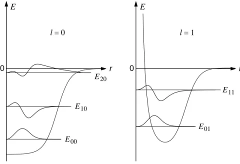
The behavior is illustrated in Figure 4 for = 0 and = 1. In the example chosen,

0 E

r l = 0

E ₀₀ E ₁₀

E ₂₀

0 E

r l = 1

E ₀₁ E ₁₁

Figure 4: Discrete states for = 0 and = 1 in the attractive potential. In the example shown are three bound states for = 0, two for = 1. The radial functions u _E = r R _E are also shown for each state. If one of the allowed energies E _n for = 1 happens to coincide with one of the energies for = 0, this would be an example of an accidental degeneracy. As pointed out in the text, such degeneracies are sometimes a consequence of the symmetry properties of the Hamiltonian.

which is that of a rather shallow short-range potential, it so happens that there are three states with = 0 and two with = 1. At the other extreme, when the potential is deep and long-range, as for the Coulomb potential, it turns out that there are infinitely many discrete, bound states for every value of , as we shall see.

4 Some Examples

We now consider a few special examples of motion in spherically symmetric potentials.

a. Spherically symmetric states ( = 0 ).

For spherically symmetric states, that is states with = 0, and hence with zero angular momentum, equation (37) reduces to

− ¯ h ² 2 m

d ² u _E0

d r ² + V ( r ) u _E0 = E u _E0

where u _E0 ( r ) satisfies the boundary condition u _E0 ( r = 0) = 0 .

Hence the problem is exactly equivalent to that of finding the odd states characterizing one-dimensional motion in the symmetrical potential

V (| x |) = V ( r ) .

The situation is particularly simple because of the absence of the invariably serious complications associated with the centrifugal potential.

As a first example, consider the states in a spherical square well potential. This example is quite important because it happens to give a fair description of the very short range interaction between a neutron and a proton in the deuteron. Such a potential is given by

V ( r ) =

− V ₀ r ≤ a 0 r > a.

The corresponding one-dimensional potential is then V ( x ) =

− V ₀ | x | ≤ a 0 | x | > a

that is, a symmetrical square well of width 2 a . We have already considered this problem in detail in Chapter VI. Among other things, we found that no bound state exists unless

V ₀ ≥ π 2

₂ h ¯ ² 2 ma ² .

Now it turns out that the deuteron has only one bound state, and that this state is rather weakly bound. Hence V ₀ exceeds this minimum value by just a little. The range of nuclear forces is known to be about 1 . 9 × 10 ⁻¹³ cm. Accepting this value for a , the depth of the potential can thus be estimated and turns out to be something like 40 MeV. Interestingly enough, this simple argument actually provided the first reliable value for the strength of nuclear forces.

b. Harmonic oscillator.

As a second example, consider the three-dimensional isotropic oscillator. Of course, we have already given a complete solutions to this problem in rectangular coordinates, but it is instructive to re-examine the problem in spherical coordinates. The = 0 states are at once simply the odd states of the one-dimensional oscillator, and hence have energies 3¯ hω/ 2, 7¯ hω/ 2, 11¯ hω/ 2 and so on. Recall now that the complete spectrum of the three-dimensional oscillator was found to be expressible as

E _n = n + 3 2

¯ hω

where the n th state was ( n + 2)( n + 1) / 2-fold degenerate. We thus see that the n th state contains among its ( n + 2)( n + 1) / 2 degenerate members, exactly one spherically symmetric state if n is even, none if n is odd. It is possible to show, although we shall not attempt to do so here, that states of higher angular momentum appear in the spectrum in the following way; For = 1, the allowed energies are 5¯ hω/ 2, 9¯ hω/ 2, · · ·;

for = 2, the allowed energies are 7¯ hω/ 2, 11¯ hω/ 2, · · ·; and so on. In general, for angular momentum , the allowed energies are ( + 3 / 2)¯ hω , ( + 2 + 3 / 2)¯ hω , ( + 4 + 3 / 2)¯ hω ,

· · ·. Otherwise stated, the degenerate members of the n th energy state are those states of angular momentum = n, n − 2 , n − 4 , · · · and so on down to = 0, for even n , or to = 1 for odd n . The spectrum, classified according to angular momentum, is shown

Energy in units of h ω

0.0 1.0 2.0 3.0 4.0 5.0 6.0

l = 0 l = 1 l = 2 l = 3 l = 4

1 3 6 10 15

Degeneracy

Figure 5: States of the three-dimensional harmonic oscillator classified accord- ing to angular momentum. The degeneracy of each state is also indicated.

in Figure 5. The degeneracy of each state in this scheme can be obtained upon noting that a state of angular momentum is 2 + 1-fold degenerate. Thus the ground state, which is = 0, is not degenerate, the first excited state which contains only an = 1 state is 3-fold degenerate, the second excited state contains a nondegenerate = 0 state and a 5-fold degenerate = 2 state so that the total degeneracy is 6-fold and so on, in agreement with our earlier rule. The pervasive occurrence of degeneracies between states of different values is an excellent example of ”accidental” degeneracies which are not accidental at all. These degeneracies occur because of the special structure of the potential for the isotropic harmonic oscillator which makes Schr¨oding equation separable in both rectangular and spherical coordinates.

c. Motion of a free particle.

We have already discussed the states of a free particle in rectangular coordinates. The

states so obtained were simultaneous eigenfunctions of the Hamiltonian and of the linear

momentum. In spherical coordinates we obtain states which are instead simultaneous

eigenfunctions of H and of the angular momentum, that is they have definite values of

E , and m . The radial functions are solutions of equation (32) with V ( r ) set equal to

zero. They thus satisfy, 1 r ²

d d r

r ² d R _E d r

+

k ² − ( + 1) r ²

R _E = 0 (39)

where

k ² = 2 mE

¯

h ² . (40)

Alternatively, these solutions may be obtained from equation (37) which, for a free particle, can be written in the form

d ² u _E d r ² +

k ² − ( + 1) r ²

u _E = 0 (41)

where, it is recalled, u _E = r R _E .

Consider first the case = 0. From equation (41), recalling that u _E must vanish ata the origin, we have at once

u _E0 ∼ sin kr and hence

R _E0 ∼ sin kr r .

For different from zero the solution is more complicated. However, it turns out that the solutions of equation (39) are a well-studied set of functions which can be compactly defined as follows:

j ( kr ) = (−1) r k

1 r

d d r

sin kr

kr . (42)

The function j ( kr ) is called a spherical Bessel function of order . In terms of these functions, and up to a multiplicative constant, the radial free particle states are given by

R _E ( r ) = j ( kr ) , k =

√ 2 mE

¯

h (43)

which clearly reduce to the correct solution for = 0. The proof that for general values the functions defined by equation (42) are actually solutions of equation (39) is not difficult, but we shall not bother to carry it out.

From equation (42) the first few spherical Bessel functions are readily found to be, j ₀ ( kr ) = sin kr

kr j ₁ ( kr ) = sin kr

( kr ) ² − cos kr kr j ₂ ( kr ) =

3

( kr ) ³ − 1 kr

sin kr − 3

( kr ) ² cos kr

(44)

which is sufficient to illustrate the general structure of these functions. Also from

equation (42), it is not difficult to obtain the explicit behavior of j ( kr ) when r is very

small and also when r is very large. In the former case, expanding sin kr / kr in a power series in kr , it is seen that the first contributing term in the series is that in ( kr ) ² , and we thus find,

r → 0 , j ( kr ) ≈ 2 !

(2 + 1)! ( kr ) . (45)

In the latter case, the dominant term is that inversely proportional to r , and we even- tually find,

r → ∞ , j ( kr ) ≈ sin( kr − π/ 2)

kr . (46)

The solutions are thus simple spherical waves at large distances from the origin. Near the origin, however, the centrifugal barrier dominates and the wave function is seen to become smaller and smaller in that region as increases.

As a simple example involving free particle states of definite angular momentum, we briefly consider the states of a particle confined in a spherical container of radius a . The wave function must vanish at the walls of the sphere and hence the spectrum of allowed energies is determined by the transcendental equation.

j ( ka ) = 0; = 0 , 1 , 2 , · · ·

For = 0, we see from equation (44) that this reduces to the simple requirement that sin ka = 0 which means that ka must simply be an integral multiple of π . For = 1, the situation is not quite so simple, since w must solve tan ka = ka , which can only be done numerically. Evidently, the equations rapidly become more and more complicated as increases, and accordingly we shall not discuss them further.

One highly interesting and important aspect of our results remains to be discussed.

We found in Section 1, that the stationary states of a free particle could be written as simple de Broglie waves corresponding to definite, but arbitrarily oriented, vector momentum p, as expressed by equation (13). Writing

p = ¯ hk n

where n

is a unit vector along p, equation (13) becomes ψ

= exp ik n

· r . (47)

On the other hand, we have just seen that for any and m ,

ψ _Em = j ( kr ) Y _m ( θ, φ ) (48)

is also a free-particle wave function corresponding to the same energy. These two

representations are complimentary in that the former describes stationary states of

well-defined linear momentum but poorly defined angular momentum while the latter

conversely describes states of well-defined angular momentum but poorly defined linear

momentum. Classically, of course, free particle states are such that both are precisely

defined. That this is not so quantum mechanically is no accident but a direct conse- quence of the easily verifiable noncommutativity of the linear and angular momentum operators.

The representations of equation (47) and equation (48) are both complete in that an arbitrary free particle state of energy E can be expressed as a superposition of either.

In particular then, each must be expressible in terms of the other. Using standard properties of the spherical harmonics and spherical Bessel functions, it can be shown after some effort that

ψ

(r) = 4 π

m

i Y _m ^∗ ( θ _p , φ _p ) ψ _Em ( r, θ, φ ) (49) where θ _p and φ _p define the angular orientation of p in the same way that θ and φ define the angular orientation of r. Conversely, in view of the orthonormality of the spherical harmonics,

ψ _Em ( r, θ, φ ) = 1 4 πi

Y _m ( θ _p , φ _p ) ψ

(r) d Ω

(50)

where d Ω

= sin θ _p d θ _p d φ _p is the element of solid angle about the unit vector n

. For a given energy, equation (49) is seen to express a state of linear momentum p as a superposition over all angular momentum states while equation (50) expresses a state of definite angular momentum as a superposition over all orientations of the linear momentum.

An important special case of equation (49) is that in which n

lies along the z -axis, the polar axis of the spherical coordinate system, so that θ _p = 0. Since

Y _m (0 , φ ) =

2 + 1 4 π δ _m0 , we obtain, upon inserting the explicit forms of ψ

and ψ _Em

ψ

= e ^{ikr cos θ} = ^∞

=0

i (2 + 1) j ( kr ) P (cos θ ) (51) where we have also used the fact that, according to equation (30),

Y _,m=0 ( θ, φ ) =

2 + 1

4 π P (cos θ )

with P (cos θ ) denoting the ordinary Legendre polynomials. Now, because the linear

momentum has been chose to lie along the z -axis, the z -component of angular momen-

tum must be zero, and so we have found; the superposition of equation (51) involves

only states with m equal to zero.

5 Hydrogen Atom

We now obtain the stationary states of a system consisting of a single electron and an atomic nucleus in purely electrostatic interaction. Denoting the magnitude of the electronic charge by e , and considering a nucleus of atomic number Z , and hence of charge Ze , the electrostatic potential is taken to be

V ( r ) = − Ze ² r .

For Z = 1 this system is the hydrogen atom, for Z = 2 it is singly ionized helium, for Z = 3 it is doubly ionized lithium, and so on. Such systems are called hydrogenic because of their obvious similarity to the hydrogen atom. Note that we have written the Coulomb potential appropriate to point charges since this is an excellent approximation on the atomic scale of distances.

We must now solve the radial equation, for a state of given angular momentum ,

− d ² u _E d r ² +

− Ze ²

r + ( + 1)¯ h ² 2 mr ²

u _E = E u _E . (52) Recall that m is the reduced mass of the system and thus is given by

m = m _e m _n m _e + m _n

where m _e is the mass of the electron and m _n that of the nucleus. Of course m differs from m _e by less than one part of a thousand but the measurements of atomic spectra are sufficiently precise that the reduced mass effect is actually detectable.

It is convenient to introduce a dimensionless coordinate y and a dimensionless bind- ing energy W , by writing

r = ¯ h ²

me ² y, E = − me ⁴

2¯ h ² W (53)

whence equation (52) takes on the much simpler form, d ² u _E

d y ² −

− 2 Z

y + ( + 1) y ²

u _E = 0 (54)

and it is this equation we must now solve. We shall do so by the proper series method.

Note first however, that for sufficiently large value of y the square bracket in equation (54) differs only slightly form W . Hence, asymptotically the behavior of u _E is dom- inated by the exponetial factor e ^{± √ W y} . Physical admissibility demands the negative sign and hence we write

u _E = v _E e ^{− √ W y} . (55)

Substitution into equation (54) then yields d ² v _E

d y ² − 2 √

W d v _E d y −

( + 1) y ² − 2 Z

y

v _E = 0 . (56) Next we determine the behavior of v _E near the origin. For this purpose, write

v _E ∼ y ^s . Substitution into equation (56) then gives

s ( s − 1) y ^s−2 − 2 √

W sy ^s−1 − ( + 1) y ^s−2 + 2 Zy ^s−1 = 0 or

s ( s − 1) − ( + 1) + 2 y ( Z − √

W ) = 0 .

the last term is negligible for sufficiently small y and hence s must be such that s ( s − 1) = ( + 1)

or

s = + 1 , − .

Since v _E must be bounded at the origin only the former is permitted and we thus see that

y → 0 , v _E ∼ y ⁺¹ .

Consequently, we now seek a power series solution of the form v _E = y ⁺¹

∞ q=0

c _q y ^q . (57)

Substitution into equation (56) then gives

∞ q=0

c _q ( q + + 1)( q + ) y ^q++1 − 2 √ W

∞ q=0

c _q ( q + + 1) y ^q+

− ^∞

q=0

c _q ( + 1) y ^q++1 + 2 Z

∞ q=0

c _q √

W ( q + + 1) − Z y ^q+ = 0 or collecting terms, we can write

∞ q=0

c _q q q + (2 + 1) y ^q++1 = ^∞

q=0

c _q √

W ( q + + 1) − Z y ^q+ . Equating coefficients of like powers of y , we then at once obtain

c _q+1 = 2

√ W ( q + + 1) − Z

( q + 1)( q + 2 + 2) c _q . (58)