2 DOF Adaptive PID Control with a Parallel Feedforward Compensator for Nonlinear Systems

2 DOF Adaptive PID Control with a Parallel Feedforward Compensator for Nonlinear Systems

Ikuro Mizumoto* and H. Tanaka Department of Intelligent Mechanical Systems

Kumamoto University

2-39-1 Kurokami, Kumamoto, 860-8555, Japan

*[email protected]

Zenta Iwai

Kumamoto Prefectural College of Technology 4455-1 Haramizu, Kikuyo-mach, Kikuchi-gun

Kumamoto, 869-1102, Japan

[email protected]

Abstract— In this paper, we propose a design method of an adaptive PID controller based on output feedback for nonlinear systems with a higher order relative degree and disturbances. To realize an adaptive PID control system, we introduce a PFC for a nonlinear system which does not satisfy OFEP(Output Feedback Exponentially Passive) conditions and design an adaptive feedforward input with a structure of RBF (Radial Basis Fuction) neural networks in order to remove the steady-state bias error from the PFC output. The proposed method can design a robust adaptive PID controller with higher accuracy on tracking control.

I. INTRODUCTION

In the recent decade, much attention has been paid to high gain output feedback-based adaptive controls for nonlinear systems due to their simple structure and high robustness with respect to uncertainties and disturbances [1], [2], [3].

The most typical design condition for designing the output feedback-based adaptive control is recognized as the output feedback exponentially passive (OFEP) condition [3]. This condition is well known as the ASPR condition for linear systems [4]. Unlike other adaptive methods, under OFEP (or ASPR) condition, one can easily design an output feedback- based adaptive controller without a priori information of the order of the controlled system and without designing a state observer.

Recently, auto-tuning and an adaptive PID control strate- gies based on the almost strictly positive real (ASPR) prop- erty of the controlled system have been proposed [8], [9] for linear systems. The PID control is one of the most common control schemes applied to many industrial processes and mechanical systems. Since the control has played a very important role in the improvement of production quality, accuracy and in reducing production costs, a great deal of attention has been turned to auto-tuning PIDs including self-tuning schemes and adaptive control strategies [5], [6], [7], [8], [9], [10] in order to maintain the desired control performance and stability during operation.

In this paper, we propose an adaptive PID control system design scheme for nonlinear systems utilizing the output feedback exponential passivity (OFEP) [3], [11] of the con- trolled system. The sufficient conditions for the system to be OFEP are that (1) the system is globally exponential minimum-phase, (2) the system has a relative degree of 1 and (3) the nonlinearities of the system satisfy the Lipschitz con- ditions [3]. Unfortunately, however, most practical systems

do not satisfy the above-mentioned OFEP conditions. In the proposed method, the introduction of a parallel feedforward compensator (PFC) is considered to solve both the relative degree and minimum-phase problems simultaneously [11], [12]. Further, since it has been indicated that affects from the introduced PFC result in degradation of the control perfor- mance in the output tracking control, we consider introducing a feedforward signal generated by an adaptive RBF NN (radial basis function neural networks) [13] directly to the original controlled system in order to maintain the output tracking control performance. The proposed adaptive PID controller can maintain stability a better control performance even if there are some changes of the system properties by adjusting PID parameters and RBF NN parameters adap- tively.

II. PROBLEM STATEMENT

Consider the following SISO affine nonlinear systems:

˙

x(t) = f(x) +g(x)u(t) +p(ω)

y(t) = h(x) (1)

where x(t) ∈ Rⁿ is a state vector, u(t) ∈ R is a control input, y(t)∈R is an output, and, f(x),g(x) :Rⁿ →Rⁿ, h(x) : Rⁿ → R are of sufficiently smooth (e.g. of class C^∞) functions such thatf(0) =0, h(0) = 0. Further,p(ω) represents the effect of disturbances. We assume that the disturbance and a reference signalyrwhich the output of the system is required to track are generated by the following exosystem:

˙

ω(t) =s(ω) yr(t) =py(ω)

s(0) =0, py(0) = 0, (2) where ω(t) ∈ R^q is a state vector of the exosystem. We assume that the exosystem (2) satisfies the neutral stabil- ity property [14]. That is, the linear approximation S = _∂s

∂ω

ω=0 of the vector field s(ω) at ω = 0 has all its eigenvalues on the imaginary axis.

Definition 1: (Output Feedback Exponentially Passive(OFEP))[3] The system (1) with p(0) = 0 is said to be OFEP if there exists a smooth output feedback:

u(t) =α(y) +β(y)v(t)

α(y) = 0, β(0) = 0 (3)

Proceedings of the 2009 IEEE International Conference on

Networking, Sensing and Control, Okayama, Japan, March 26-29, 2009

such that the resulting closed loop system fromv(t)toy(t) is exponentially passive, that is for the closed loop system, the following dissipation inequality (DI) is satisfied

V˙(x) =∂V(x)

∂x (f(x) +g(x)v)≤yv−ζ(x) (4) with a (C²) positive definite function V and a positive definite functionζ(x)having the following properties:

δ1||x||²≤V(x)≤δ2||x||²

δ3||x||²≤ζ(x), (5) where δ1∼δ3 are positive constants andζ(x)is a positive definite function.

Sufficient conditions for the system (1) to be OFEP have been provided in [3] such that (C1) the system has a relative degree of one, (C2) the system be globally exponential minimum-phase and (C3) the nonlinearities of the system satisfy the Lipschitz condition.

In this paper, we consider an adaptive PID control system design based on the OFEP property for nonlinear systems which do not satisfy OFEP conditions.

We suppose that the nominal part of the system (1) satisfies the following assumptions.

Assumption 1: The system (1) has a relative degree of r and there exists a nonsingular transformation z(t) = [z1, z2,· · ·, zn]^T = Φ(x) such that the system (1) can be transformed into the following canonical form:

˙

zi(t) = zi+1(t) +pi(ω) (i= 1,2,· · · , r−1)

˙

zr(t) = a(zξ,η) +b(zξ,η)u(t) +pr(ω)

˙

η(t) = q(zξ,η) +p_η(ω) y(t) = z1(t)

(6)

where zξ= [z1,· · ·, zr]^T,η= [zr+1,· · ·, zn]^T and a(0,0) =L^r_fh(0) = 0, q(0,0) =0

b(zξ,η) =LgL^r_f⁻¹h(x)= 0, ∀x∈Rⁿ

Assumption 2: Nonlinear functions a(zξ,η), q(zξ,η) andb(zξ,η)are globally Lipschitz with respect to(zξ,η).

Assumption 3: There exist positive constantsB¯M and¯b0

such thatb(zξ,η)can be evaluated as

0<¯b0≤b(z_ξ,η)≤B¯M (7) Assumption 4: The linear approximation of the system (1) at x(t) = 0 is stabilizable and its zero dynamics has no eigenvalue on the imaginary axis.

The objective of this paper is to design a PID control system which has the outputy(t) track the reference signal yr(t) for uncertain nonlinear systems with higher order relative degrees and/or non-minimum phase properties. That is, for uncertain nonlinear systems, the goal is to achieve

tlim→∞|y(t)−yr(t)| ≤δ (8) for any given small positive constant δ.

III. CONTROL SYSTEM DESIGN

It has been clarified that, under Assumption 4 and the as- sumption that the exosystem (2) satisfies the neutral stability property, there exists an ideal statex^∗(t)and an ideal input v^∗(t)which attain perfect output tracking:

˙

x^∗(t) =f(x^∗) +g(x^∗)v^∗(t) +p(ω)

y(t) =yr(t) =h(x^∗) (9) and they are given by functions ofω as x^∗(t) =π(ω)and v^∗(t) =c(ω)[14], [15].

In the following, we will show an adaptive PID control system design with the adaptively estimated feedforward input v(t) of the ideal input v^∗(t) for uncertain and non- OFEP systems.

A. Ideal Input Approximation by RBF NN

Consider approximating the ideal control input v^∗(t) by a Radial Basis Function (RBF) neural networks (NN). We approximatev^∗(t)by the form of RBF NN as

vnn(t) =W^TS(ω) (10) where W = [w1,· · ·, wl]^T ∈ R^l is the weight vector, l is the number of NN nodes (weight number) and S(ω) = [s1(ω),· · · , sl(ω)]^T is the radial basis function vector. This basis function vector S(ω) is generally designed by the Gaussian functions such as

si(ω) = exp

−(ω−μ_i)^T(ω−μ_i) ηi²

, i= 1,2,· · ·, l (11) where μ_i = [μi1,· · ·, μiq]^T is the center of the receptive field andηi is the width of the Gaussian function.

It has been clarified [13] that, for a sufficiently largeland a compact setΩω⊂R^q, there exists an ideal constant weight vectorW^∗ such that

W^∗arg min

W∈R^l

sup

ω∈Ω_ω|v^∗−W^TS(ω)|

(12) and thus the ideal inputv^∗(t)can be approximated by

v^∗(t) =W^∗TS(ω) + (ω)

| (ω)| ≤ ^∗ (13) where (ω)is an approximation error.

Here we impose the following assumption.

Assumption 5: For a given NN nodes l, there exists an ideal weight vectorW^∗ that satisfies (12) for allω∈Ωω.

In practice,W^∗is the unknown vector so that one can not designW in (10) asW =W^∗.W will be adaptively adjust in the proposed control system design which will be shown later.

B. Realization of OFEP controlled system

In order to guarantee the stability of the designed adaptive PID control system, we consider utilizing system’s OFEP property. Unfortunately, however, most practical systems including those with relative degree of greater than 1 and/or non-minimum phase are not OFEP, we here consider an introduction of a parallel feedforward compensator (PFC) to realize an OFEP augmented controlled system [11], [12].

Consider anfth order PFC of the form:

˙

xf(t) =Afxf(t) +bfu(t)

yf(t) =c^T_fx_f(t) (14) and introduce this in parallel with the system (1). The resulting augmented system can be represented by

˙

x(t) =f(x) +g(x)u(t) +p(ω)

˙

xf(t) =Afxf(t) +bfu(t)

ya(t) =y(t) +yf(t) =h(x) +c^T_fxf(t). (15) Since the augmented system (15) has a relative degree of 1, there exists a nonsingular transformation [ya,η_a] = Φa(x,xf) such that the augmented system (15) can be transformed into the following form [14]:

˙

ya(t) =aa(ya,η_a) +ba(ya,η_a)u(t) +p1(ω)

˙

η_a(t) =q_a(ya,η_a) +p_ηa(ω) (16) Here we impose the following assumption on the aug- mented system (16).

Assumption 6: The zero dynamics of the augmented sys- tem (16):

˙

η_a(t) =q_a(0,η_a) (17) is exponentially stable.

Assumption 7: The PFC (14) is strictly positive real (SPR).

It should be noted that, under Assumption 2, aa(ya,η_a), q_a(ya,η_a) and ba(ya,η_a) are globally Lipschiz and thus under Assumption 6, the resulting augmented system is OFEP [3]. That is, we assume that an SPR PFC which render the resulting augmented system OFEP is known.

Furthermore, under assumption 3, it follows that there exist positive constantsBM andb0 such that

0< b0≤ba(ya,η_a)≤BM (18) C. Adaptive PID System Design

Adaptive PID controller with adaptive NN feedforward input is designed as follows:

u(t) =ue(t) +v(t) ue(t) =−K(t)^TZ(t)

v(t) = ˆW^T(t)S(ω)

(19) with

K(t) = [kp(t), kd(t), ki(t)]^T, Z(t) = [¯ea(t),e˙¯a(t), w(t)]^T

˙

w(t) = ¯ea(t)−δw(t), δ >0

(20)

＋－ ＋＋

Adaptive NN Controller

PFC Nonlinear-System Reference

Model

Adaptive PID ω v

( ) ( ) ( ) ( )ω

ω ω s

p t y

t

r =

& = yr e_a u_e u

( ) ( ) ( )

( )^t ( )^t y

t u t A t

f T f f

e f f f f

x c

b x x

= +

& =

yf

y ya

( ) ( ) ( ) ( ) ( ) ( ) ( )^{fxx gx pω}

x h t y

t u t

=

+ +

& =

＋－ ＋＋

Adaptive NN Controller

PFC Nonlinear-System Reference

Model

Adaptive PID ω v

( ) ( ) ( ) ( )ω

ω ω s

p t y

t

r =

& = yr e_a u_e u

( ) ( ) ( )

( )^t ( )^t y

t u t A t

f T f f

e f f f f

x c

b x x

= +

& =

yf

y ya

( ) ( ) ( ) ( ) ( ) ( ) ( )^{fxx gx pω}

x h t y

t u t

=

+ +

& =

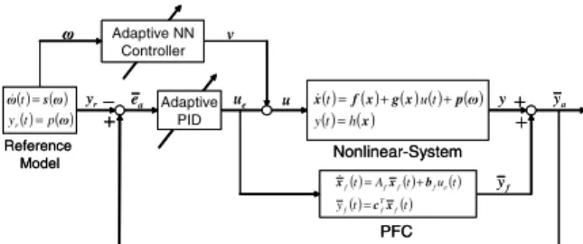
Fig. 1. Block diagram of the proposed adaptive control system

and

k˙p(t) = γpe¯²a(t)−σpkp(t), γp>0, σp>0 k˙d(t) = γde¯a(t) ˙¯ea(t)−σdkd(t), γd>0, σd>0 k˙i(t) = γie¯aw(t)−σiki(t), γi>0, σi>0 W˙ˆ(t) = −ΓS(ω)−σWˆ(t), Γ>0, σ >0

(21)

Where

¯

ea= ¯ya(t)−yr(t) (22)

¯

ya(t) =y(t) + ¯yf(t) (23) andy¯f(t)is defined as the output of the PFC withue(t)as an input

˙¯

xf(t) =Afx¯f(t) +bfue(t)

¯

yf(t) =c^T_fx¯f(t). (24) Wˆ(t)is an estimated value of the ideal weight vectorW^∗.

The overall block diagram of the designed control system is shown in Fig. 1

D. Stability Analysis

Equivalent representation of the designed control system given in Fig. 1 is given by the following form using the augmented system representation given in (16)

˙

ya(t) =aa(ya,η_a) +ba(ya,η_a)(ue(t) +v(t)) +p1(ω)

˙

η_a(t) =q(ya,η_a) +p_ηa(ω)

¯

ya(t) =ya(t)−yˆf^∗(t), (25) where yˆ^∗f(t)is a PFC output withv(t)as an input

˙ˆ

xf(t) =Afxˆf(t) +bfv(t) ˆ

y^∗f(t) =c^T_fxˆf(t) (26) Further, the ideal state in which the perfect output tracking y(t)≡yr(t)is achieved is also represented as follows using the augmented system expression.

˙

ya^∗(t) =aa(y^∗a,η^∗_a) +ba(ya^∗,η^∗_a)v^∗(t) +p1(ω)

˙

η^∗_a(t) =q(ya^∗,η^∗_a) +p_ηa(ω)

¯

ya^∗(t) =yr(t) =y^∗a(t)−y^∗f(t),

(27) wherey^∗f(t)is a PFC output with the ideal feedforward input v^∗(t)as an input.

˙

x^∗_f(t) =Afx^∗_f(t) +bfv^∗(t)

yf^∗(t) =c^T_fx^∗_f(t) (28)

From(25)and(27), the error system can be represented by Δ ˙ya =aa(ya,η_a)−aa(y^∗a,η^∗_a)

+ba(ya,η_a)(ue(t) +v(t))−ba(ya^∗,η^∗_a)v^∗(t) Δ ˙η_a =q_a(ya,η_a)−q_a(ya^∗,η^∗_a) (29)

¯

ea(t) = ¯ya(t)−y¯^∗a= Δya−Δyf^∗,

where Δya = ya(t)−ya^∗(t), Δη_a = η_a(t)−η^∗_a(t) and Δy^∗f = ˆy^∗f(t)−yf^∗(t).

Next considering the difference between (26) and (28), we have the following PFC error system:

Δ ˙xf =AfΔxf+bfΔv

Δyf^∗ =c^T_fΔxf, (30) where Δxf = ˆxf(t)−x^∗_f(t)andΔv=v(t)−v^∗(t).

From Assumption 7, the PFC error system (30) can be transformed into the following canonical form:

Δ ˙y^∗f =ayΔy^∗f+c^T_yη_y+byΔv

˙

η_y =Aη_yη_y+cη_yΔyf^∗

(31) using an appropriate nonsingular transformation [14].

Therefore it follows from (29) and (31) that the error system can be rewritten as

˙¯

ea =aa(ya,η_a)−aa(y^∗a,η^∗_a)

+ba(ya,η_a)(Δue+ Δv−K^∗TZ) +(ba(ya,η_a)−ba(ya^∗,η^∗_a))v^∗

−ayΔyf^∗−c^T_yη_y−byΔv Δ ˙η_a =q_a(ya,η_a)−q_a(ya^∗,η^∗_a)

˙

η_y =Aη_yη_y+cη_yΔyf^∗

(32)

where

Δue=ue(t)−u^∗e(t) =−K^T(t)Z+K^∗TZ

=−ΔK^TZ (33)

ΔK^T = [Δkp,Δkd,Δki]^T

= [kp(t)−k^∗p, kd(t)−kd^∗, ki(t)−ki^∗]^T Δv =v(t)−v^∗(t) = ˆW^T(t)S(ω)−W^∗TS(ω)−

= Δ ˆW^TS(ω)− (34) From Assumption 6, there exist a positive definite functionU(Δη_a) and positive constants κ1 to κ4 such that [16]

∂U(Δη_a)

∂η_a q_a(0,Δη_a)≤ −κ1Δη_a² ∂U(Δη_a)

∂η_a

≤κ2Δη_a κ4Δη_a²≤U(Δη_a)≤κ3Δη_a².

(35)

Further since the PFC error system (31) is SPR from Assumption 7, representing(31)as

Δ ˙¯xf = ¯AfΔ¯xf+ ¯bfΔv Δyf^∗ = ¯c^T_fΔ¯xf

(36) with

Δ¯xf = [Δy^∗f,η^T_y]^T A¯f =

ay c^T_y cη_y Aη_y

,¯bf =

by

0

¯

c^T_f = [1,0,· · · ,0]

there exist positive definite matrices P¯f = ¯P_f^T > 0,Q¯f = Q¯^Tf >0such that the following Kalman-Yakubovich Lemma is satisfied

A¯fP¯f+ ¯PfA¯f=−Q¯f

P¯f¯bf = ¯cf. (37) Now, consider a positive definite functionV:

V =Ve+Vη+δ1Vx_f +Vk

+(BM +by)Δ ˆW^TΓ⁻¹Δ ˆW (38) withVe = ¯e²a, Vη =μ1U(Δη_a), Vx_f = Δ¯x^T_fP¯fΔ¯xf, Vk =

b0

γ_pΔkp2+_γ^b0_dΔkd2+^b_γ⁰_iΔki2+b0ki^∗w²+b0k^∗de¯²a and any positive constantδ1, μ1.

The time derivative ofVe= ¯e²acan be evaluated from(32) that

V˙e= 2¯ea{aa(ya,η_a)−aa(ya^∗,η^∗_a) +ba(ya,η_a)(Δue

+Δv−K^∗TZ) + (ba(ya,η_a)−ba(ya^∗,η^∗_a))v^∗

−ayΔyf^∗−c^T_yη_y−byΔv}

≤2¯ea{La1(|Δya|+Δη_a) +ba(ya,η_a)(Δue

+Δv−K^∗TZ) +bMv^∗−ayΔy^∗f

−c^T_yη_y−byΔv}.

WhereLa1is a Lipschiz constant such that

aa(ya,η_a)−aa(ya^∗,η^∗_a)< La1(|ya−ya^∗|+η_a−η^∗_a) andbM is a positive constant that satisfies

0<ba(ya,η_a)−ba(ya^∗,η^∗_a) ≤bM

The time derivative ofVη=μ1U(Δη_a)can be evaluated as

V˙η =μ1∂U

∂η_a{q_a(ya,η_a)−q_a(y^∗a,η^∗_a)}

≤μ1∂U

∂η_aq_a(0,Δη_a) +μ1

∂U

∂η_a

(q_a(ya,η_a)

−q_a(0,Δη_a)) +μ1

∂U

∂η_a

q_a(y^∗a,η^∗_a)

≤ −μ1κ1Δη_a²+μ1κ2Δη_aLq(|ya|+η^∗_a) +μ1κ2Δη_aqM

WhereLq is a Lipschiz constant such that

q_a(ya,η_a)−q_a(0,Δη_a)< Lq(|ya|+η^∗_a) andqM is a positive constant that satisfies

0<q_a(ya^∗,η^∗_a) ≤qM.

Further the time derivative ofVx_f = Δ¯x^T_fP¯fΔ¯xf can be evaluated as

V˙x_f = ( ¯AfΔ¯xf+ ¯bfΔv)^TP¯fΔ¯xf

+ Δ¯x^T_fP¯f( ¯AfΔ¯xf+ ¯bfΔv)

=−Δ¯x^T_fQ¯fΔ¯xf+ 2Δy^∗fΔv

≤ −λQ_fΔ¯xf²+ 2Δy^∗fΔv

≤ −1

2λQ_f|Δyf^∗|²−1

2λQ_fη_y²+ 2Δy^∗fΔv

≤ −(1

2λQ_f −ρy)|Δyf^∗|²−1

2λQ_fη_y²+ 1 ρy

|Δv|², (39) where λQ_f = λmin[ ¯Qf] is the minimum value of the eigenvalues ofQ¯f andρy is any positive constant.

Furthermore for Vk we have V˙k = 2b0

γp

Δkp(γp¯e²a−σpkp) +2b0

γd

Δkd(γde¯ae˙¯a−σdkd) +2b0

γi Δki(γie¯aw−σiki) + 2b0k^∗iw(¯ea−δw) +2b0k^∗de¯ae˙¯a

= 2b0Δkp¯e²a−2b0σp

γp

Δkpkp+ 2b0Δkd¯eae˙¯a

−2b0σd

γd Δkdkd+ 2b0Δkie¯aw−2b0σi

γi Δkiki

+2b0k^∗iw¯ea−2b0ki^∗δw²+ 2b0kd^∗¯eae˙¯a, (40) Thus, the time derivative ofV is evaluated by

V˙ = ˙Ve+ ˙Vη+δ1V˙xf+ ˙Vk

+(BM+by)(−ΓS(ω)¯ea−σWˆ)^TΓ⁻¹Δ ˆW +(BM+by)Δ ˆW^TΓ⁻¹(−ΓS(ω)¯ea−σWˆ)

≤2La1|¯ea||Δya|+ 2La1|¯ea|Δη_a −2b0kp^∗¯e²a

+2bM|¯ea||v^∗|+ 2ay|Δyf^∗||¯ea|+ 2|¯ea|c_yη_y

−μ1κ1Δη_a²+μ1κ2LqΔη_a(|¯ea+ Δyf^∗+y^∗a| +η^∗_a) +μ1κ2qMΔη_a −δ1(1

2λQ_f −ρy)|Δy^∗f|²

−δ1

2λQ_fη_y²+ δ1

ρy(Δ ˆW²S(ω)²

+2 ^∗Δ ˆWS(ω)+ ^∗2) + 2(BM+by) ^∗|e¯a|

−2b0σp

γp |Δkp|²+2b0σp

γp |Δkp||k^∗p|

−2b0σd

γd |Δkd|²+2b0σd

γd |Δkd||kd^∗|

−2b0σi

γi

|Δki|²+2b0σi

γi

|Δki||ki^∗| −2b0δ|k^∗i|w²

−2(BM+by)σλΓΔ ˆW²

+2(BM+by)σλ^MΓ Δ ˆWW^∗, (41) where, λΓ = λmin[Γ⁻¹] and λ^M_Γ = λmax[Γ⁻¹] are the minimum and the maximum values of the eigenvalue ofΓ⁻¹.

Consequently, we have V˙ ≤ − 2b0kp^∗−2La1−L²a1

ρ0 −L²a1

ρ1 −ρ2−a²y

ρ3 −cy² ρ4

−μ²1κ²2L²q

4ρ6 −ρ13

|¯ea|²

−(μ1κ1−ρ1−ρ5−ρ6−ρ7−ρ8−ρ9)Δη_a²

− δ(1

2λQ_f −ρy)−ρ0−ρ3−μ²1κ²2L²q

4ρ7

|Δy^∗f|²

− δ1

2λQ_f −ρ4

η_y²− 2b0σp

γp −ρ10

|Δkp|²

− 2b0σd

γd

−ρ11

|Δkd|²− 2b0σi

γi

−ρ12

|Δki|²

− 2(BM+by)σλΓ−ρ14−ρw

−δ1

ρyS²M

Δ ˆW²−2b0δ|ki^∗|w²+b²M|v^∗|² ρ2

+μ²1κ²2L²q

4ρ5 η^∗_a²+μ²1κ²2L²q

4ρ8 |ya^∗|²+μ²1κ²2

4ρ9 q²M

+b²0σ²p

γp²ρ10|kp^∗|²+ b²0σd²

γd²ρ11|k^∗d|²+ b²0σi²

γi²ρ12|ki^∗|² +δ1²SM²

ρwρ²y

∗²+δ²1

ρy

∗²+(BM +by)² ρ13

∗²

+(BM+by)²σ²λ^MΓ ²

ρ14 W^∗2 (42)

with any positive constants ρ0 ∼ ρ14, ρw and SM = maxS(ω). Then, considering a sufficiently large ideal feedback gaink^∗ such that

2b0k^∗p−2La1−^L_ρ^2a₀¹ −^L_ρ^2a₁¹ −ρ2−^a_ρ^2y₃

−c_y²

ρ4 −^μ21_4ρ^κ226^L2q −ρ13

> γν >0 (43)

and settingρ0,ρ1,ρ3 ∼ρ12,ρ12,ρy,ρw,δ1,μ1 such as ρ1 =ρ5=ρ6=ρ7=ρ8=ρ9=^μ1₇^κ1

ρy = ^λQf₄ , ρ0=ρ3= ^δ₁₆¹λQ_f, ρ4=³¹₆₄δ1λQ_f

ρ10= ^b0_γ^σ_p^p, ρ11= ^b0_γ^σ_d^d, ρ12=^b0_γ^σ_iⁱ ρ14=ρw= ^(BM+b₂^y)σλΓ

δ1 = ^16μ_λ^1κ22L2q

Qfκ1 , μ1= ^{(BM+by)σλΓκ1λ}

2 Qf

128κ²2L²_qS_M² ,

we have

V˙ ≤ −γν|¯ea|²−1

7μ1κ1Δη_a²− δ1

64λQ_fΔ¯xf²

−b0σp

γp |Δkp|²−b0σd

γd |Δkd|²−b0σi

γi |Δki|²

−1

2(BM +by)σλΓΔ ˆW²−2b0δ|k^∗i|w²+R (44)