Multi-Colored Rooted Tree Analysis of the Weak Order Conditions of a Stochastic Runge-Kutta Family under a

CSSE-22 October 8, 2004

Multi-Colored Rooted Tree Analysis of the Weak Order Conditions of a Stochastic Runge-Kutta Family under a

Commutativity Condition

Yoshio Komori

Department of Systems Innovation and Informatics Kyushu Institute of Technology

680-4 Kawazu Iizuka, 820-8502, Japan [email protected]

Abstract

The present paper is aimed at multi-colored rooted tree analysis to give a trans-

parent expression of weak order conditions of a stochastic Runge-Kutta family for

stochastic dierential equations satisfying a commutativity condition. As a result, a

new explicit stochastic Runge-Kutta scheme is given, which is of weak order 2 and

order 4 in the deterministic mean.

1 Introduction

Stochastic dierential equations (SDEs) appear to make mathematical models in many elds 7, 13]. Since SDEs are analytically unsolvable in most cases, however, numerical methods for SDEs have been studied by many researchers.

The methods are categorized into two types based on the meaning of approximation.

One type provides an approximate solution in the mean square sense 3]. The other type provides an approximation in the weak sense. The present paper deals with the latter.

Many numerical methods in the weak sense (weak schemes) have been proposed for multi-dimensional SDEs with multiplicative noise in the multi-dimensional Wiener process case. Let us introduce results concerning the schemes that attains weak order 2 for such SDEs. Klauder and Petersen 6] have proposed a weak scheme in the sense dened by the separation of an approximate solution into its deterministic and stochastic parts. Milstein 10] and Tocino and Ardanuy 15] have proposed weak schemes with derivatives of the drift or the diusion coecients. Kloeden and Platen 7, 11] have proposed a derivative-free scheme by replacing necessary derivatives of higher order by nite dierences of higher order. On the other hand, Roler 12] has proposed other derivative-free schemes by assuming a commutativity condition 1, 14].

The paper 12] has disclosed the important fact that schemes with only the random variables corresponding to the increment of Wiener process can attain weak order 2 under the commutativity condition. This will lead to our scheme given in Section 4 of the present paper.

As we can see in the papers mentioned above, the calculation to derive weak order conditions is a troublesome task in general. The rooted tree analysis for ordinary dif- ferential equations (ODEs) by Butcher 4, 5] can, however, become a help to relieve the task. In fact, Komori 8] has extended it to obtain weak order conditions of a stochastic Runge-Kutta family for SDEs with a multi-dimensional Wiener process. By utilizing the results, we will transparently get weak conditions under the commutativity condition in the later section.

The aim of the present paper is to show the analysis of weak order conditions under the commutativity condition, and give an explicit stochastic Runge-Kutta scheme of weak order 2.

Next, let us introduce the denition of weak (global) order. For the d -dimensional stochastic integral equation

y

( t ) =

^y0

+

^Z

^t

0 g

0

(

^y

( s ))d s +

^X

^m

j

⁼¹

Z

t

0

g

j (

^y

( s )) d W j ( s ) 0

t

T end

where W j ( s ) is a scalar Wiener process and means the Stratonovich formulation, we give equidistant grid points n

^def

= nh ( n = 0 1 ::: M ) with step size h

^def

= T end =M < 1 ( M is a natural number) and consider discrete approximations

^y

_n to

^y

( n ). Let C _lP (

^R

^d

^R

) denote the totality of l times continuously dierentiable

^R

-valued functions on

^R

^d , all of whose partial derivatives of order less than or equal to l have polynomial growth. Then, the denition is given as follows 2].

De nition 1.1 Suppose that discrete approximations

^y

_n are given by a scheme. Then, we say that the scheme is of weak (global) order q if for each G

²

C _P

²⁽

^q

⁺¹⁾

(

^R

^d

^R

),

⁹

C > 0 (independent of h ) and > 0 such that

j

E G (

^y

( M )]

^;

E G (

^y

_M )]

^j

Ch ^q h

²

(0 ) :

1

The organization of the present paper is as follows. In Section 2 we will give a general expression of weak order conditions for a stochastic Runge-Kutta family by the extended rooted tree analysis. In Section 3 we will give a similar expression under the commuta- tivity condition. In Section 4 we will nd a solution of the order conditions after giving simplifying assumptions, and give some numerical experiments under the commutativity conditions. In Section 5 we will give the summary. In the appendix, we will show the expectations of elementary weights and elementary numerical weights for weak order 2.

2 Weak order conditions by multi-colored rooted trees

The aim in this section is to express weak order conditions by multi-colored rooted trees.

Because the theoretical content like proof has been already given in 8], we only give here the brief introduction to the expression of weak order conditions.

2.1 The Stratonovich-Taylor expansion for the stochastic dier- ential equation solution

The purpose of this subsection is to represent the truncated Stratonovich-Taylor expansion of

y

( n

⁺¹

) =

^y

_n +

^{Z n+1}

n g

0

(

^y

( s ))d s +

^X

^m

j

⁼¹

Z

n+1

n

g

j (

^y

( s )) d W j ( s ) (2. 1) by functions on the set of multi-colored rooted trees (MRTs).

Let us suppose that any component of the d -vector valued function

^g

_j belongs to C _P

²

^q (

^R

^d

^R

) (0

j

m ), and denote by

^y2

_q ( n

⁺¹

) the truncated expansion of

^y

( n

⁺¹

) satisfying ( x ) + ( x )

2 q , where ( x ) means the multiplicity of integrals with respect to a time variable or Wiener processes, and ( x ) means the multiplicity of integrals with respect to a time variable for a multiple stochastic integral x appearing in the expansion.

First, we are to introduce MRT.

De nition 2.1 (Multi-colored rooted tree (MRT) ) A multi-colored rooted tree with a root

^jg

(colored with a label j from 0 to m ) is a tree recursively dened in the following way.

1)

⁽

^j

⁾

is the primitive tree having only a vertex

^jg

.

2) If t

¹

::: t k are multi-colored trees, then t

¹

::: t k ]

⁽

^j

⁾

is also a multi-colored rooted tree with the root

^jg

.

The totality of MRTs is denoted by T:

t

^{1 q q q}

t k

q q q

J J J J

g

j

Figure 1: Generation of the tree t

¹

::: t k ]

⁽

^j

⁾

2

Next, let ( t ) be the number of vertices of t

²

T , r ( t ) the number of vertices of t with the color 0, and ( t ) the number of dierent ways of numbering on t in the way that along each outwardly directed arc the numbers increase and vertices of a subtree are consecutively numbered. (See Fig. 2.)

g

l

4

g

j

3

g

2

l J J

g

j

1

g

l

3

g

j

2

g

4

l J J

g

j

1

Figure 2: Examples of numbering on t

Furthermore, we introduce an integral operator and three functions on T . For any integrable function H of

^y

and s > n ,

J

⁰

H ]( s )

^def

=

^Z

^s

n

H (

^y

( s

¹

))d s

¹

J j H ]( s )

^def

=

^Z

^s

n

H (

^y

( s

¹

)) d W j ( s

¹

)

(1

j

m ). In the sequel, it is clear that the upper bound of integral interval is n

⁺¹

only with respect to the last integral variable in the multiple integrals. Thus, we will omit this symbol for ease of notation.

De nition 2.2 (Elementary weight ⁽ t ) on T ) An elementary weight of t

²

T is given recursively as follows.

(

⁽

^j

⁾

) = J j 1] ( t ) = J j

"

k

Y

i

⁼¹

( t i )

#

for t = t

¹

::: t k ]

⁽

^j

⁾

:

De nition 2.3 (Elementary dierential

^F

^{( t )} on ^T ) An elementary di erential is a possibly multilinear operator recursively given as follows.

F

(

⁽

^j

⁾

) =

^g

_j (

^y

_n )

F

( t ) =

^g(

_j ^k

⁾

(

^y

_n )

^F

( t

¹

) :::

^F

( t k )] for t = t

¹

::: t k ]

⁽

^j

⁾

:

De nition 2.4 (Elementary coecient ^{( t )} on ^T ) ^{The index ( t ) ( t}

²

^{T ) is dened}

recursively.

(

⁽

^j

⁾

) = 1 ( t ) = 1 k !

k

Y

i

⁼¹

( t i ) for t = t

¹

::: t k ]

⁽

^j

⁾

: Note that 0

j

m in these denitions.

Then, we obtain one of the important results.

Theorem 2.1 The nitely truncated expansion has the following expression.

y

2

q ( n

⁺¹

) =

^y

n +

^X2

^q

i

⁼¹

X

⁽

t

⁾⁺

t

²

r T

⁽

t

⁾⁼

i

( t ) ( t )

^F

( t )( t ) :

3

2.2 The Taylor expansion for a stochastic Runge-Kutta family

In order to obtain an approximate solution

^y

_n

⁺¹

of the solution

^y

( t n

⁺¹

) of (2. 1), we consider the stochastic Runge-Kutta family given by

y

n

⁺¹

=

^y

_n +

^X

^s

i

⁼¹

m

X

j

⁼⁰

c

⁽

_i ^j

^)Y(

_i ^j

⁾

Y (

j

^a)

i

^a

=

^X

^m

j

^b=0

i

^(a

^j

^a

^j

^b)

8

<

:

b

⁽

i ^j

^aa

^j

^b)g

j

^b

(

^y

n +

^X

^s

i

^b=1

m

X

j

^c=0

⁽

i

^a

^j

^a

i

^b

^j

^b

^j

^c)Y(

j

^c)

i

^b

) +

^g(1)

_j

^b

(

^y

_n )

^X

^s

i

^b=1

m

X

j

^c=0

_i

^(a

^j

^a

_i

^b

^j

^b

^j

^c)Y(

_i

^b

^j

^c)

9

=

(2. 2)

(1

i a

s , 0

j a

m ), where each _i

^(a

^j

^a

^j

^b)

is a random variable independent of

^y

_n and satises

E

_i

^(a

^j

^a

^j

^b)2

^k

=

(

K

¹

h

²

^k ( j b = 0) K

²

h ^k ( j b

⁶

= 0)

for constants K

¹

, K

²

and k = 1 2 ::: . If b

⁽

_i

^a

^j

^a

^j

^{b) 6}

= 0, by setting ~

⁽

_i

^a

^j

^a

^j

^{b) def}

= _i

^(a

^j

^a

^j

^b)

b

⁽

_i

^a

^j

^a

^j

^b)

and ~ _i

^(a

^j

^a

_i

^b

^j

^b

^j

^{c) def}

=

⁽

_i

^a

^j

^a

_i

^b

^j

^b

^j

^c)

=b

⁽

_i

^a

^j

^a

^j

^b)

we can rewrite this in the following simpler form:

y

n

⁺¹

=

^y

_n +

^X

^s

i

⁼¹

m

X

j

⁼⁰

c

⁽

i ^j

^)Y(

j

⁾

i

Y (

j

^a)

i

^a

=

^X

^m

j

^b=0

~ i

^(a

^j

^a

^j

^b)

8

<

:

g

j

^b

(

^y

_n +

^X

^s

i

^b=1

m

X

j

^c=0

⁽

i

^a

^j

^a

i

^b

^j

^b

^j

^c)Y(

j

^c)

i

^b

) +

^g(1)

_j

^b

(

^y

_n )

^X

^s

i

^b=1

m

X

j

^c=0

~ i

^(a

^j

^a

i

^b

^j

^b

^j

^c)Y(

j

^c)

i

^b

9

=

(2. 3)

(1

i a

s , 0

j a

m ). Note that these formulations include stochastic Rosenbrock- Wanner methods 9].

In this section we deal with the simple formulation and represent the truncated Taylor expansion of

^y

_n

⁺¹

centered at

^y

_n by functions on the set of multi-colored rooted tree with labels (MRTL).

Let us denote by

^y

_n

⁺¹

²

_q the truncated expansion of

^y

_n

⁺¹

satisfying ( x ) + ( x )

2 q , where ( x ) means the multiplicity of products with respect to ~ _i

^(a

⁾

, and ( x ) means the multiplicity of products with respect to ~ _i

^(a

⁾

except ~

⁽

_i

^a

⁰⁾

for a monomial x of ~ _i

^(a

⁾

appearing in the expansion.

First, we introduce several matrices related to the formula parameters of (2. 3). Let us dene

A

⁽

^j

^{) def}

=

2

6

6

6

6

6

6

6

6

6

6

6

6

6

6

6

6

6

4

¹¹⁽⁰

^j

⁰⁾

⁽¹¹

^mj

⁰⁾

⁽⁰

s

⁺¹

^j

⁰⁾¹

⁽

s ^mj

⁺¹

¹⁰⁾

... ... ... ... ... ... ...

⁽⁰¹¹

^jm

⁾

¹¹⁽

^mjm

⁾

⁽⁰

s

⁺¹

^jm

¹⁾

⁽

s ^mjm

⁺¹

^{1 )}

... ... ... ... ... ... ...

¹⁽⁰

_s ^j

⁰⁾

⁽¹

^mj _s

⁰⁾

⁽⁰

_s

⁺¹

^j _s

⁰⁾

⁽

_s ^mj

⁺¹

_s

⁰⁾

... ... ... ... ... ... ...

⁽⁰¹

_s ^jm

⁾

¹⁽

^mjm _s

⁾

⁽⁰

_s

⁺¹

^jm _s

⁾

⁽

_s ^mjm

⁺¹

_s

⁾

0

0

0

0

3

7

7

7

7

7

7

7

7

7

7

7

7

7

7

7

7

7

5

4

for

⁽

_i

^a

^j

^a

_i

^b

^j

^b

^j

^c)

. Similarly, dene the matrix ~;

⁽

^j

⁾

for ~ _i

^(a

^j

^a

_i

^b

^j

^b

^j

^c)

, and set ~ A

⁽

^j

^{) def}

= A

⁽

^j

⁾

+ ~;

⁽

^j

⁾

. In addition, dene the ( m + 1)( s + 1)

( m + 1)( s + 1) diagonal matrix D

⁽

^j

⁾

by

D

⁽

^j

^{) def}

= diag(~

¹⁽⁰

^j

⁾

~

¹⁽

^mj

⁾

~

⁽⁰

s

⁺¹

^j

⁾

~

⁽

s ^mj

⁺¹⁾

) : Next, we introduce MRTL and a function on its set.

De nition 2.5 (Multi-colored rooted tree with labels (MRTL)) A multi-colored rooted tree with labels, denoted by t X , is one attached by labels according to the following rule.

1) The label of the root is X .

2) The label of the other vertices is decided by the number of branches and the color of the parent vertex:

the label is ~ A

⁽

^j

⁾

if the parent vertex has a single branch and is colored with j .

the label is A

⁽

^j

⁾

if the parent vertex has more than one branch and is colored with j .

The totality of MRTL's whose roots are labeled with X , is denoted by

^T

X . For example, some MRTL's are listed in Fig. 3.

g

j

A

⁽⁰⁾

g

j

A

⁽

^j

⁾

g

A

⁽

^j

⁾ l J J

g

j

A

⁽⁰⁾

g

l

A ~

⁽

^l

⁾

g

l

A ~

⁽

^j

⁾

g

j

A

⁽⁰⁾

Figure 3: Examples of trees in

^T

A

⁽⁰⁾

De nition 2.6 (Elementary numerical weight ^{( t )} on

^T

^X ) An elementary numer- ical weight of t

^2T

X is given recursively as follows.

( _X

⁽

^j

⁾

) = 1 D

⁽

^j

⁾

X ( t ) = (

^Y

^k

i

⁼¹

( t i )) D

⁽

^j

⁾

X for t = t

¹

::: t k ]

⁽

_X ^j

⁾

(0

j

m ), where 1 stands for an ( m + 1)( s + 1)-dimensional row vector of 1's, and

Q

ki

⁼¹

( t i ) means the elementwise product of row vectors ( t i ).

Then, we obtain another important result.

Theorem 2.2 The nitely truncated expansion of the numerical solution by the stochastic Runge-Kutta family has the following expression.

y

n

⁺¹

²

q =

^y

_n +

^X2

^q

i

⁼¹

X

^{(^}

t

⁾⁺

r

^{(^}

t

⁾⁼

i t

^2TA

(0)

(^ t ) (^ t )

^F

(^ t )

⁽

m

⁺¹⁾

s

⁺¹

( t ) :

where

⁽

m

⁺¹⁾

s

⁺¹

( t ) denotes the (( m + 1) s + 1)-st element of ( t ) and ^ t means an MRT obtained by removing all labels from t

^2T

_A

⁽⁰⁾

.

5

2.3 Order conditions of the stochastic Runge-Kutta family

We give the transparent way of seeking the order conditions by utilizing the multi-colored rooted tree analysis.

Let us suppose the sucient smoothness of g j 's and the regularity of the time dis- crete approximation. Then, the condition concerning convergence order in the important theorem presented by Platen 7, 11] can be rewritten as follows 8]: there exist constants K <

¹

and r

^{2 f}

1 2 :::

^g

independent of h such that for all n = 0 ::: M

^;

1 and ( p

¹

::: p L )

^2f

1 ::: d

^g

^L (1

L

2 q + 1),

E

2

4

L

Y

j

⁼¹

(

^y

n

^+1;y

n ) p

^{j; Y}

L

j

⁼¹

(

^y2

q ( n

⁺¹

)

^;y

n ) p

^j

F

n

3

5

K (1 + max

0

k

n

^jy

k

^j2

r ) h ^q

⁺¹

(w : p : 1) : (2. 4) Here, (

^z

) p

^j

and

^F

n denote, respectively, the p j -th component of

^z

and a non-anticipating sub- -algebra generated by the discretized Wiener processes W j ( i )'s (0

i

n 1

j

m ). If (2. 4) is satised, the time discrete approximation

^y

_M converges to the

^y

( M ) with weak (global) order q as h

^!

0.

Furthermore, let us rewrite (2. 4) by utilizing the multi-colored tree expression. We can replace

^y

_n

^+1;y

_n in (2. 4) with

^y

_n

⁺¹

²

_q

^;y

_n by noting that any term in the expansion of

^y

_n

^+1;y

_n

⁺¹

²

_q centered at

^y

_n does not prevent the inequality from holding. After the replacement, the substitution of the results in Theorems 2.1 and 2.2 into the expression in the left-hand side of (2. 4) yields

E

2

6

6

6

6

4

L

Y

j

⁼¹

(

^X2

^q

i

⁼¹

X

^{(^}

t

⁾⁺

r

^{(^}

t

⁾⁼

i t

^2TA

(0)

(^ t ) (^ t )

^F

(^ t )

⁽

m

⁺¹⁾

s

⁺¹

( t )) p

^j

;

L

Y

j

⁼¹

(

^X2

^q

i

⁼¹

X

⁽

t

⁾⁺

r

⁽

t

⁾⁼

i t

²

T

( t ) ( t )

^F

( t )( t )) p

^j

F

n

3

7

7

7

5

=

^X2

^q

i

¹⁼¹

X

^{(^}

t

¹⁾⁺

r

^{(^}

t

¹⁾⁼

i

¹

t

^12TA

(0)

2

q

X

i

^L=1

X

⁽

t

^{^L)+}

r

^{(^}

t

^L)=

i

^L

t

^L2TA

(0)

L

Y

j

⁼¹

( (^ t j ) (^ t j )(

^F

(^ t j )) p

^j

)

E

2

4

L

Y

j

⁼¹

⁽

_m

⁺¹⁾

_s

⁺¹

( t j )

^;Y

^L

j

⁼¹

(^ t j )

F

n

3

5

(w.p.1) : Eventually, since ~

⁽

_i

^a

^j

^b)

is independent of

^y

_n , (2. 4) holds if the condition

E

2

4

L

Y

j

⁼¹

⁽

m

⁺¹⁾

s

⁺¹

( t j )

3

5

= E

2

4

L

Y

j

⁼¹

(^ t j )

3

5

(2. 5)

follows for any t

¹

::: t L

^2T

A

⁽⁰⁾

satisfying

^P

_Lj

⁼¹

( (^ t j ) + r (^ t j ))

2 q .

Next, we show a way of seeking the expectation in the right-hand side of (2. 5) with the help of MRTs. In the multiple Stratonovich integrals, the usual chain rule holds as in the deterministic case. Hence, we can rewrite the product of elementary weights or the composition of subtrees in a elementary weight by the following:

6

The product of elementary weights of two MRTs t

¹

, t

²

can be expressed by the sum of elementary weights of an MRT generated by grafting t

¹

to the root of t

²

and an MRT generated by grafting t

²

to the root of t

¹

.

The elementary weight of an MRT having subtrees t

¹

, t

²

can be expressed by the sum of elementary weights of an MRT generated by grafting t

¹

to t

²

's own root and an MRT generated by grafting t

²

to t

¹

's own root.

For example, we have

(

^0g

)

^ljgg

=

g

l

g

j

g

0

!

+

^0gj^glg

=

g

l

g

j

g

0

!

+

g

l

g

0

g

j

!

+

g

0

g

l

g

0

!

:

In addition, by utilizing the relationship between multiple Stratonovich integrals and multiple It^o integrals (11], p. 173), we can rewrite the expectations of MRTs whose each vertex has no more than one branch as follows:

The expectation of an elementary weight vanishes unless the even number of vertices are of colors dierent from 0 and each of these vertices has a parent or child vertex with the same color.

The expectation of an elementary weight of an MRT in which a vertex has a parent or child vertex with the same color is equal to a half of that of another MRT given by replacing the two vertices with one vertex with the color 0. For example,

E

"

g

j

g

j

g

0

!#

= 12 E

^00gg

= 12

^00gg

:

Note that there is no longer need of the expectation in the right-hand side.

In this way we obtain the expectations of elementary weights or the products of them in Appendix A.

Next, we give a way of seeking the expectations in the left-hand side of (2. 5) with the help of MRTL's. From the observation of calculations for some elementary numerical weights according to Denition 2.6, we can see that the (( m + 1) s + 1)-st element of an elementary numerical weight can be obtained directly from a diagram for an MRTL by the following procedure.

Trace vertices in the direction from the root to upper vertices.

For the root vertex, prepare indices i

¹

and j

¹⁰

and write down c

⁽

i ^j

¹¹⁰⁾

. Then, write down ~ _i

⁽¹

^j

¹⁰

^j

⁾

if the color is j .

For each vertex except the root, prepare new indices i k

⁺¹

and j _k

⁰⁺¹

and write down

⁽

_i

^k

^j

^k0

_i

^{k +1}

^jj

^{k +10 )}

if the label is A

⁽

^j

⁾

, or ~

⁽

_i

^k

^j

^k0

_i

^{k +1}

^jj

^{0k +1)def}

=

⁽

_i

^k

^j

^k0

_i

^{k +1}

^jj

^{k +10 )}

+~ _i

^(k

^j

^k

_i

^{0k +1}

^jj

^{k +10 )}

if it is ~ A

⁽

^j

⁾

, where i k and j _k

⁰

mean the indices of the parent vertex. Then, write down ~ _i

^{(k +1}

^j

^{k +10}

^l

⁾

if the color is l .

Finally, sum over all values (1 ::: s ) and (0 ::: m ) of all indices in relation to i and j

⁰

, respectively.

7

For example,

⁽

m

⁺¹⁾

s

⁺¹

g

0

~

A (j)

g

jA (0)

=

^X

^s

i

¹

i

²⁼¹

m

X

j

⁰¹

j

⁰²⁼⁰

c

⁽

_i ^j

¹⁰¹⁾

~ _i

⁽¹

^j

¹⁰

^j

⁾

~

⁽

_i ^j

¹⁰¹

_i

²

^jj

²⁰⁾

~

⁽

_i

²

^j

²⁰

⁰⁾

: Now, let us assume the following.

Assumption 2.1 The expectation of the (( m + 1) s + 1)-st element of an elementary numerical weight or the product of those is equal to 0 if the odd number of vertices are of the same color j (

⁶

= 0).

Then, we can obtain the expectations of the (( m + 1) s + 1)-st elements of elementary numerical weights or the products of them for weak order 2 as in Appendix B.

3 Weak order conditions in a commutative case

In the previous section we have shown the expression of weak order conditions by MRTL's.

In this section we will obtain a similar expression under a commutativity condition.

3.1 Special case

In general, if elements t

¹

, t

²

in T dier in the structure or in the coloring,

^F

( t

¹

)

⁶

=

^F

( t

²

) holds. Before the commutative case, we consider the expression of order conditions in a special case that

^F

( t ) is equivalent for some t 's whose structures are the same but whose colorings dier.

Suppose that

^F

( t ) is equivalent for the t 's under an assumption O . As preliminaries, we dene a subset of T , say T O , such that

for each t

²

T , an element u in T O exists and satises

^F

( t ) =

^F

( u ),

for elements u

¹

, u

²

in T O , when they dier in the coloring even if they are the same in the structure,

^F

( u

¹

)

⁶

=

^F

( u

²

) holds.

In addition, we set

V u

^def

=

^f

t

^jF

( t ) =

^F

( u ) t

²

T

^g

for u

²

T O . Then, from Theorem 2.1 we obtain

y

2

q ( n

⁺¹

) =

^y

_n +

^X2

^q

i

⁼¹

X

⁽

u

⁾⁺

u

²

r T

^(O

u

⁾⁼

i

( u ) ( u )

^F

( u )

8

<

: X

t

²

Vu ( t )

9

=

(3. 1) by noting that ( t ) and ( t ) do not depend on the coloring of t

²

V u .

Similarly, we dene a subset of

^T

X , say

^T

XO , such that

for each t

^2T

X , an element u in

^T

XO exists and satises

^F

(^ t ) =

^F

(^ u ),

for elements u

¹

, u

²

in

^T

XO , when they dier in the coloring even if they are the same in the structure,

^F

(^ u

¹

)

⁶

=

^F

(^ u

²

) holds,

8

and set

V

Xu

^def

=

^f

t

^jF

(^ t ) =

^F

(^ u ) t

^2T

X

^g

for u

^2T

XO . Then, from Theorem 2.2 we obtain

y

n

⁺¹

²

q =

^y

_n +

^X2

^q

i

⁼¹

X

⁽

u

⁾⁺

r

⁽

u

⁾⁼

i u

^2TA

(0)

O

(^ u ) (^ u )

^F

(^ u )

8

>

<

>

: X

t

^2VA

(0)

u

⁽

m

⁺¹⁾

s

⁺¹

( t )

9

>

=

>

: (3. 2)

As in Subsection 2.3, from (2. 4), (3. 1) and (3. 2) we can see that (2. 4) holds if the condition

E

2

6

4

L

Y

j

⁼¹

8

>

<

>

: X

t

^2VA

(0)

u

^j

⁽

m

⁺¹⁾

s

⁺¹

( t )

9

>

=

>

3

7

5

= E

2

6

4

L

Y

j

⁼¹

8

>

<

>

: X

t

^2VA

(0)

u

^j

(^ t )

9

>

=

>

3

7

5

(3. 3)

holds for any u

¹

::: u L

^2T

A

⁽⁰⁾

O (1

L

2 q ) satisfying

^P

_Lj

⁼¹

( (^ u j ) + r (^ u j ))

2 q .

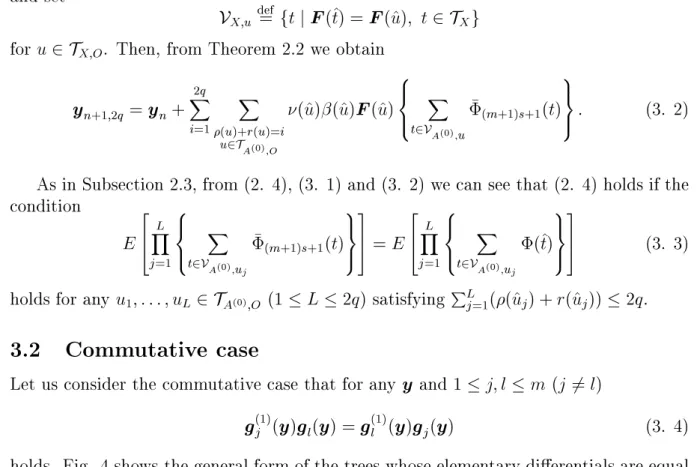
3.2 Commutative case

Let us consider the commutative case that for any

^y

and 1

j l

m ( j

⁶

= l )

g

(1)

j (

^y

)

^g

_l (

^y

) =

^g(1)

_l (

^y

)

^g

_j (

^y

) (3. 4) holds. Fig. 4 shows the general form of the trees whose elementary dierentials are equal under this commutativity condition. The big triangles stand for a common MRT.

g

l

g

j

J

J

J J

g

j

g

l

J

J

J J

Figure 4: Generation of equivalent trees under the commutativity condition Let us adopt the commutativity condition as O in the previous subsection. Among the MRTL's shown in Appendix B, we can choose those in Table 1 as v

^2T

_A

⁽⁰⁾

_O for which the number of elements in

^V

A

⁽⁰⁾

v is greater than 1.

Table 1: Elements in

^V

_A

⁽⁰⁾

v

i 1 2 3 4

v i

g

l

~

A (j)

g

j

~

A (l)

g

l

~

A (j)

g

jA (0)

g

l

~

A (j)

g

jA (j)

g

l A

(j)

g

jA (0)

g

l

~

A (j)

g

j

~

A (j)

g

jA (0)

g

l

~

A (j)

g

jA (0)

We are interested in combinations of MRTL's for which both sides of (3. 3) do not vanish. For some of such combinations under Assumption 2.1, let us demonstrate how to

9